Effect of Compaction on Soil Physical Properties of Differently Textured Landfill Liner Materials


1
Leibniz-Centre for Agricultural Landscape Research (ZALF), Eberswalder Straße 84, 15374 Müncheberg, Germany
2
Institute of Plant Nutrition and Soil Science, Christian Albrechts University Kiel, Christian-Albrechts-Platz 4, 24118 Kiel, Germany
*
Author to whom correspondence should be addressed.
Geosciences 2019, 9(1), 1; https://doi.org/10.3390/geosciences9010001
Submission received: 31 October 2018
/
Revised: 14 December 2018
/
Accepted: 17 December 2018
/
Published: 20 December 2018
(This article belongs to the Special Issue Soil Hydrology and Erosion)
Abstract
:Mineral landfill liners require legally-fixed standards including a sufficiently-high available water capacity (AWC) and relatively low saturated hydraulic conductivity values (Ks). For testing locally available and potentially suitable materials with respect to these requirements, the soil hydraulic properties of boulder marl (bm) and marsh clay (mc) were investigated considering a defined compaction according to Proctor densities. Both materials were pre-compacted in 20 soil cores (100 cm3) each on the basis of the Proctor test results at five degrees of compaction (bm1–bm5; mc1–mc5) ranging between 1.67–2.07 g/cm3 for bm and 1.09–1.34 g/cm3 for mc. Additionally, unimodal and bimodal models were used to fit the soil water retention curve near saturation and changes in the pore size distribution (PSD). The structural peak of the PSD in the fraction of pore volume between −30 and −60 hPa was more pronounced on the dry side (bm1–2, mc1–2) than on the wet side of the Proctor curve (bm4–5, mc4–5). Therefore, the loss in structural pores can be attributed to an increasing dry bulk density for bm and an increasing gravimetric moisture content during Proctor test for mc. While the mc fulfils the legal standards with AWC values between 0.244–0.271 cm3/cm3, the Ks values for bm between 1.6 × 10⁻⁶ m/s and 3.8 × 10⁻⁷ m/s and for mc between 7.4 × 10⁻⁷ m/s and 1.2 × 10⁻⁷ m/s were up to two orders of magnitude higher than required. These results suggest that the suitability of both materials as landfill liner is restricted.
1. Introduction
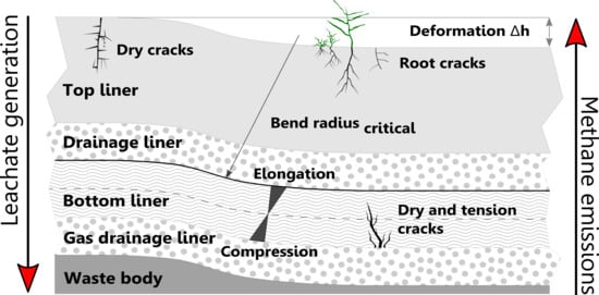
The increasing global population leads to an increasing amount of municipal waste that must be a) recycled, b) burned, or c) deposited [1]. The latter option requires legally-fixed environmental and technical standards. Therefore, the German Landfill Directive, which was enacted in 2009, includes the essential qualitative criteria for engineered barriers [2]. Landfill capping systems are essential to protect the immediate environment of the waste body that can include aromatic hydrocarbons, carbolic acids, or heavy metals (i.e., arsenic).
Therefore, capping systems are purposed to (a) protect the groundwater against potentially leaking bottom liners through leachate minimizing and (b) inhibit the diffusive emission of greenhouse gases (i.e., methane) [3]. The top and bottom liner of landfills are often constructed by natural materials (i.e., clay, boulder marl) that should fulfil the technical requirements of technical guidelines [1,2]. Natural materials can be installed in combination with geotextiles or geomembranes, although their application is restricted due to the high cost factor, especially in financially less powerful regions (i.e., Romania) as stated by reference [4]. Consequently, high engineering demands are placed on the material. Considering the legally-fixed standards, (a) plant available water capacity (AWC ≥ 0.14 cm3/cm3), (b) saturated hydraulic conductivity (Ks value ≤ 5 × 10⁹ m/s equal to 0.5 m thickness and a hydraulic gradient of i = 0.3), (c) air capacity (AC ≥ 0.08 cm3/cm3), and (d) low shrinkage tendency (volume shrinkage index < 5%) are essential soil physical properties of mineral landfill liner [5,6]. These properties were regularly affected by the degree of compaction and the water content during liner installation considering potential changes in the pore size distribution (PSD) [6,7].
The study is focused on the Rastorf landfill (Northern Germany), because the temporary installed capping system with a maximum duration of up to 10 years must be transferred into a final capping system according to the statutory requirements as mentioned before. Therefore, it was the task of the authors to estimate the soil chemical and physical characteristics of locally available and sustainable material and its possible use as landfill top and bottom liner [5]. In this case, boulder marl (bm) and marsh clay (mc) were chosen, while bm was also an integral part of the temporary capping system that, if suitable, could be continued to be used. Both substrates are also common for its use as landfill liners, even in combination with elastic polymers, depending on the hazardousness of the stored waste [1].
Proctor compaction tests [8] are requested before installation of mineral landfill liner to determine the effect of compaction on the soil water retention curve (SWRC) characteristics including AWC, AC, as well as the Ks values due to the statutory requirements in Germany. For a more accurate description of the SWRC in the near-saturated soil water content, the standard unimodal approach [9] assuming a single-porosity could be used to fit observed data from fine-textured soils, or if bimodal approaches [10] could better represent any modality of the PSD induced by soil mechanical processes in compacted liners. The impact soil shrinkage on the long-term sealing effect of mineral landfill liner was described in a previous study [6] and is excluded from the current study, but the opportunity of PSD as an indicator for the shrinkage-dependent volume change was tested for both materials.
In this context, the estimated fitting parameter (i.e., van Genuchten parameter), especially for heavily compacted soils (>1.8 g/cm3) are a useful addition towards commonly used data [11] in case of landfill engineering and modelling. The modelling process including the water and solute transport in the vadose zone, and therefore the fitting parameter, are essential to improve the modelling performance of the Rastorf landfill as mentioned by [12]. This step is necessary to make essential adjustments to the existing temporary capping system before transferring part of it into the final capping system and to construct a final capping system with proven efficiency with respect to the statutory requirements. The adjustments include, among other things, the application of compost to the chosen substrates, since its ability as soil conditioner was proven in several field and laboratory studies (i.e., [13]).
The first objective of this study was to determine the effect of compaction on the soil physical properties of boulder marl (bm) and marsh clay (mc) and its suitability as landfill liner materials considering experimental Proctor compaction tests. The second objective was to investigate the effect of compaction on the pore size distribution, and therefore the modality, to find the optimum model (unimodal or bimodal) for further water flow transport modelling of landfill liner systems. Additionally, the effect of compost application on SWRC characteristics of boulder marl was also tested to answer the question whether and how can compost improve the water holding capacity of landfills’ top liner.
The authors hypothesized that the degree of compaction affects (i) the pore size distribution and (ii) the modality of the SWRC, and therefore the soil physical properties of both materials, and that (iii) compost application positively affects the SWRC characteristics of boulder marl.
This study intends to provide knowledge on soil chemical and physical properties of alternative materials for engineering landfill capping systems.
2. Materials and Methods
The boulder marl derived from a pit located in the young moraine landscape (Rastorf: lat 54°16′ N, long 10°19′ E) and the marsh clay from decalcified marshland (Barlt: lat 54°28′ N, long 9°18′ E) in the state of Schleswig-Holstein in Northern Germany. Both materials were used for the Proctor compaction test (ASTM D-698).
In June 2013, as a result of erosion damage and less pronounced vegetative growth, approximately 100 m3 of compost, produced in the local compost facility (Rastorf, Northern Germany) consisting of tree and shrub chippings and debris, was applicated by milling machine to the upper 0.2 m of the top liner (same boulder marl for Proctor compaction tests) of the Rastorf landfill on approximately 1000 m2 [14,15]. The basic material was mechanically shredded and frayed and then stored in a composting plant for nearly 9 months to enhance the biochemical processes of composting between 70 °C and 100 °C. In 2013 (without compost: wco) and 2015 (compost: co), more than 80 undisturbed soil cores (diameter: 0.055 m, height: 0.04 m) were collected from a pit in the northeast part of the landfill (lat 54°28′ N, long 10°32′ E) in depths between 0.1 m and 0.2 m.
2.1. Standard Proctor Compaction Tests
Disturbed and homogenized bm and mc material was used for four standard Proctor compaction tests (ASTM D-698), respectively. Therefore, the material was moistened and then compacted to estimate a) the optimum dry bulk density (ρtopt) and b) the optimum water content (wopt) including two different stages at the dry side (bm1, bm2, mc1, mc2) and wet side (bm4, bm5, mc4, mc5) of the optimum water content (bm3, mc3) as mentioned following reference [6].
As result, 20 soil cores (diameter: 5.5 cm, height: 4 cm) per Proctor stage (1–5) were prepared with standard method by a load frame through a stamp (diameter: 5.5 cm) with a static load of 50 kN (Instron, Norwood, MA, USA) to estimate AC, AWC, and Ks values of both materials, respectively.
2.2. Laboratory Analyses of Soil Properties
Disturbed bm, mc, wco, and co material was used to estimate the organic carbon content (OC) with coulometry, soil texture (sieve and pipette method), soil pH (pH meter, CaCl2), particle density (ρs) (pycnometer method), and dry bulk density (ρt) (core method) with 4 replications per Proctor stage, respectively, based on standard laboratory experiments as mentioned in the following literature [16]. The Ks values were determined by the falling-head method [17] with 5 to 10 undisturbed soil cores for each Proctor stage, wco and co, respectively.
The SWRC characteristics were measured from undisturbed soil cores (5 to 10 per Proctor stage, wco, co) by a combined pressure plate (quasi-saturated, −30, −60, −150, −300, −500, −1000 hPa) and −15,000 hPa ceramic vacuum outflow method as well as oven-dried for 16 h at 105 °C [16].
The total porosity was calculated from the ratio between bulk, ρt, and solid particle density, ρs (bm: 2.63–2.64 g/cm3, mc: 2.67–2.68 g/cm3); the air capacity (AC) and the plant available water capacity (AWC) were calculated as follows:
where θ is the volumetric water content (cm3/cm3), θs is the saturated volumetric water content (cm3/cm3), and θr (cm3/cm3) is the residual water content, subscripts FC (field capacity) and PWP (permanent wilting point) indicate the water content at −60 hPa and −15,000 hPa, respectively.
2.3. Descriptions of the Soil Water Retention Curve
The software SWRC FIT [10] was used to fit the observed soil water retention data based on a Levenberg–Marquardt optimization method with the following unimodal and bimodal models: Brooks–Corey (BC) model [18], van Genuchten (VG) model [9], Fredlund and Xing (FX) model [19], Kosugi (LN) model [20], Durner (DB) model [21], and Seki (BL) model [10]. The effective water saturation, Se, is defined as follows:
The Brooks–Corey (BC) model is expressed as follows [18]:
where h is the pressure head (hPa) and hb is the pressure head value (hPa) at air-entry.
The van Genuchten (VG) model is defined as [9]:
where α is a scale parameter inversely proportional to pore diameter (1/cm), n is related to the pore size distribution with n ≥ 1, and m is the Mualem coefficient and defined as m = 1 − 1/n with 0 < m < 1.
The Fredlund and Xing (FX) model described was used as follows [19]:
where α is related to the air entry value of the soil (hPa), n is related to the maximum slope of the soil, m is related to the curvature of the slope, e is the Euler’s number (of natural exponential function), and C(h) is the correction factor that extends the range of pressure head up to 1 × 10⁷ hPa.
The linear Kosugi (LN) model [20] was used in the following form:
where hm is the capillary pressure head (hPa) related to the median pore radius (cm), σ is a dimensionless parameter related to the width of the pore radius distribution, and Q is related to the complementary error function (erfc) as follows:
where x describes the term in brackets in Equation (6).
The bimodal Durner (DB) model includes the weight term w for two VG soil water retention functions in the following formulation [21]:
In this study, the differential function for the SWRC was directly regarded as the soil PSD in form of the slope of the SWRC [23]:
According to reference [20], the boundary between the macro-pores and the structural pores (wide coarse pores, wCP) was assumed between 0 hPa and −10 hPa, while the first peak is described by the wCP; the second or third peak (matric peak) is described by textural pores (narrow coarse pores: nCP, medium pores: MP, fine pores: FP) as proposed follows reference [23].
2.4. Shrinkage Behaviour and Volume Shrinkage Index
In addition to the SWRC characteristics, the soil volume change at the different drying stages as mentioned before was estimated with the laser triangulation method as detailed described in a previous study following reference [6]. The volume shrinkage index (VSI) was also used to describe the pore size dependent shrinkage tendency defined as follows (wide coarse pores, >50 µm, 0 to −60 hPa), nCP (narrow coarse pores, 50–10 µm, −60 to −300 hPa), medium pores (MP, 10–2 µm, −300 to −15,000 hPa), and fine pores (<2 µm, <−15,000 hPa).
where ∆Vt is the soil volume in relation to the drained water-filled pore volume (∆Vp) and i corresponds to the pore size (coarse, medium, and fine pores) of the respective drying stage.
In this study, the differential function of the VSI was directly compared to the soil PSD in the following form:
2.5. Statistical Analysis
The mean values and standard deviations for each sampling depth and the correlation coefficient (r2) as index of goodness of fit were calculated. The second-order Akaike Information Criterion (AICc) for small sample sizes [24]:
where n is the effective sample size and K is the number of estimated parameters. For a specified data set, the model with the lowest AICc will be the “best” model among all models [25]. The statistical quality criteria were used to represent the deviations between the fitted (xsim) and the observed (xobs) volumetric water contents. Therefore, the higher the arithmetic mean of the absolute error, the higher is the root mean square error (RMSEθ):
3. Results
3.1. Soil Characteristics of the Tested Materials
Both materials were integral parts of further studies [5,6], thus, only the basic soil characteristics are listed in the present study. The tested materials are characterized by a sandy loam (SL) and clay loam (CL) texture with a clay content between 11 wt% and 26 wt%, respectively (Table 1). The pH values range from a moderately acidic character (pH 5.6) to a slightly alkaline character (pH 7.6); the organic carbon content (OC) of mc was significantly higher than of bm with similar ρs values, respectively. The particle densities (ρs) varied between 2.65 g/cm3 and 2.67 g/cm3.
The Proctor densities of bm were comparatively higher than of mc, while the corresponding water content is inversely proportional (Table 2).
The intermediate to firm ρt values of bm were comparatively higher than the very small ρt values of mc (Table 3). The Ks values of mc varied between 1.2 × 10⁷ m/s and 7.4 × 10⁷ m/s and those of bm between 3.8 × 10⁷ m/s and 1.2 × 10⁶ m/s (Table 3). The AC and AWC values reached the lowest level at the Proctor optimum (bm3), except the AC values of mc that decreased with increasing moisture content.
The SWRC of bm and mc for five different Proctor stages based on the unimodal and bimodal models are presented in Figure 1, while the fitting parameters are listed in Table 4 and Table 5. The Proctor optimum of the boulder marl (bm3) indicated the lowest θs, while θs of marsh clay is decreasing with increasing water content. The LN and FX models predicted slightly higher θs values than the BC and VG models, even the DB model, while the BL model had comparatively higher θs values for mc3 and mc4 than the other models. On the other side, the θs values were very close to each other.
The goodness of fit for the SWRC parameters obtained with bimodal and unimodal models are listed in Table 6. The bimodal models showed minimally higher coefficients of determination (r2 ≥ 0.98) than all unimodal SWRC. The DB model fit for the boulder marl and the BL model fit for the marsh clay were found to be best due to the more negative values of the AIC criterions as compared to all other models and for all degrees of Proctor density.
For the five different Proctor stages, the RMSEθ values of the bimodal DB and BL models were comparatively lower than for the unimodal BC, VG, LN, and FX models (Table 7). The smallest differences between fitted (xsim) and observed (xobs) θ values were found for the Proctor optimum (bm3) with 0.002 cm3/cm3 to 0.003 cm3/cm3, while mc5 on the wet side of the Proctor curve showed the lowest RMSEθ values between 0.005 cm3/cm3 and 0.015 cm3/cm3 (Table 7). Thus, the RMSEθ values of mc were up to one order of magnitude higher than the RMSEθ values of bm.
3.2. Pore Size Distribution and Modality of Both Tested Materials
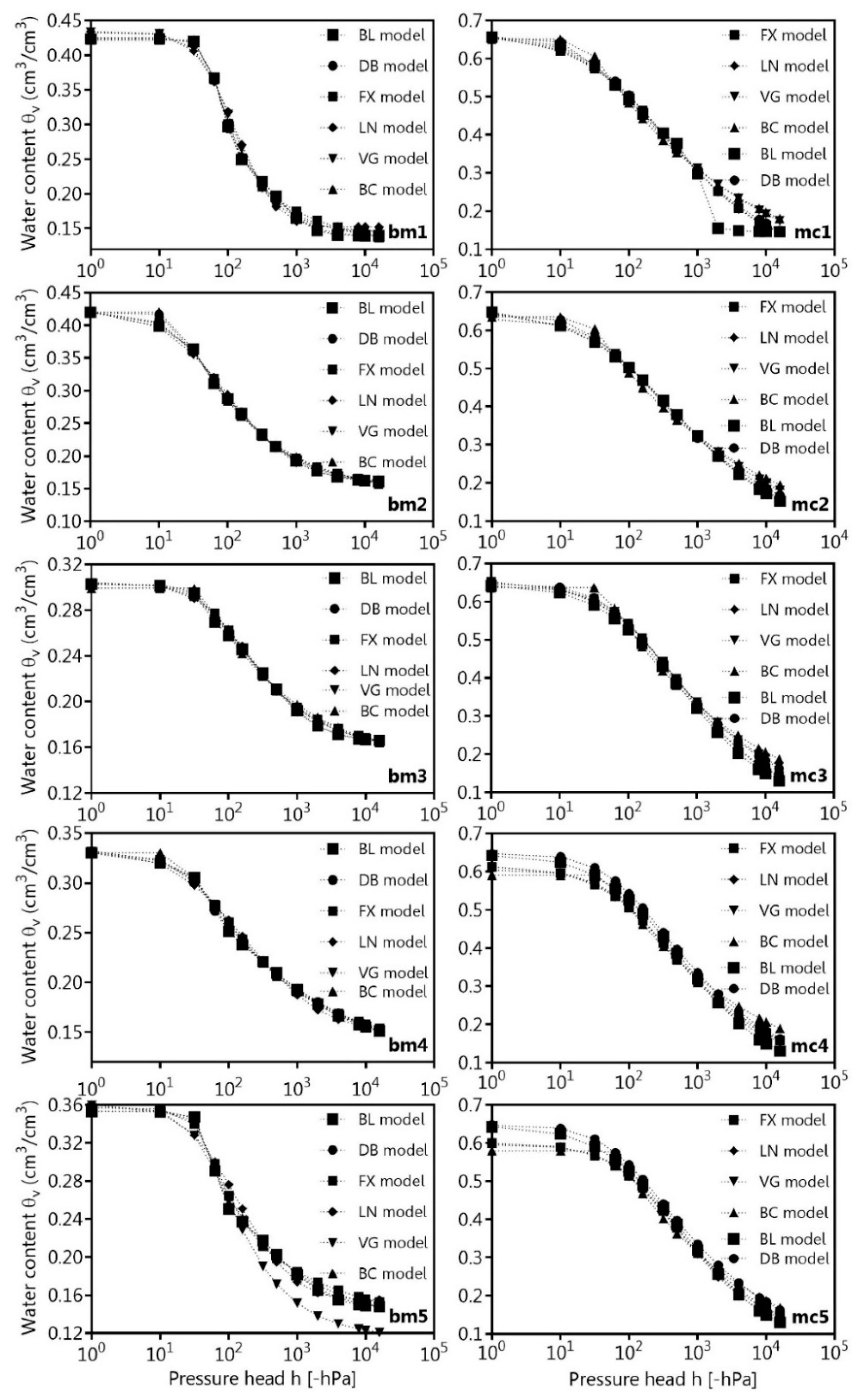
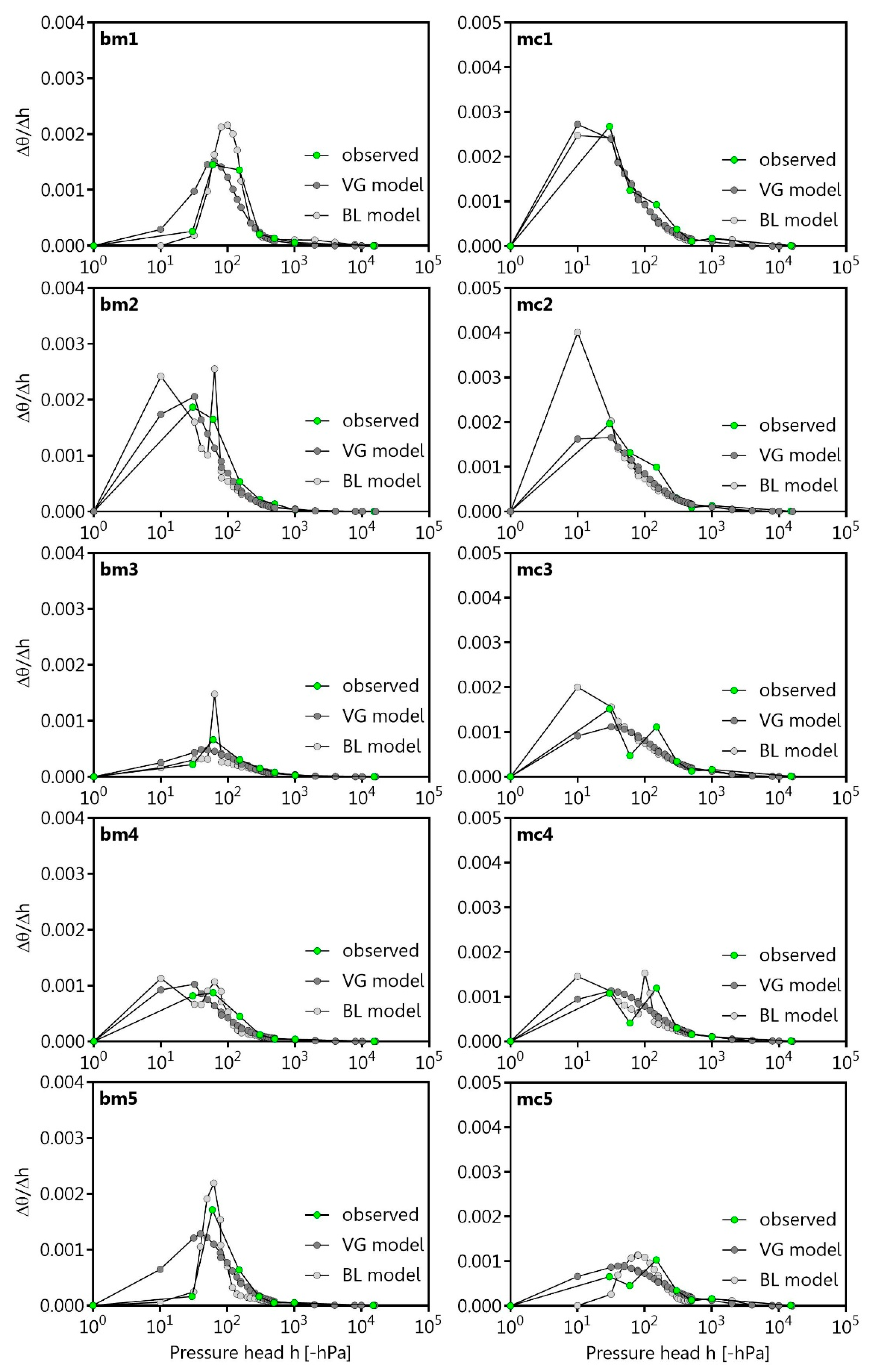
On the basis of the presented results, the authors decided to use the unimodal VG model and the bimodal BL model for further investigations of the pore size distribution (PSD). The observed and fitted PSD of bm1–bm3 were characterised by a mono-peak (structural peak) between −30 and −60 hPa. Thus, the emptying of the wCP corresponded to a pronounced water loss, even for the SWRC fitted with VG and BL models, while mc1–mc3 showed a first peak between −30 and −60 hPa and a second peak (porous matric peak) between −60 and −150 hPa as well as a mono-peak pore size distribution on the basis of the VG and BL models (Figure 2). The SWRCs describe that an emptying of structural pores here denoted as wCP (>−60 hPa) and textural pores denoted as nCP (−60 to −300 hPa) leads to a pronounced water loss.
On the other hand, bm4 showed a mono- or single-peak for the observed data and the VG model between −30 hPa and −60 hPa, and a bi-or double-peak structure for the BL model SWRC with a more pronounced second peak between −60 and −150 hPa, just as mc4. Additionally, bm5 is characterised by an observed and fitted mono-peak PSD, while the observed data of mc showed a triple-peak PSD (structural and matric peaks) with peaks at −30 hPa and −150 hPa as well as a less pronounced peak at −1000 hPa. Thus, the medium pores (−300 to −15,000 hPa) is related to significant soil water storage fraction, which, however, is still smaller than that of wCP and nCP (Figure 2). There are more pronounced differences between the observed data and the fits of bimodal SWRC models for wCP, nCP, and FP, especially for mc3 and mc4; thus, the bi-double-peaked PSD was not well described by the VG and BL model (Table 8).
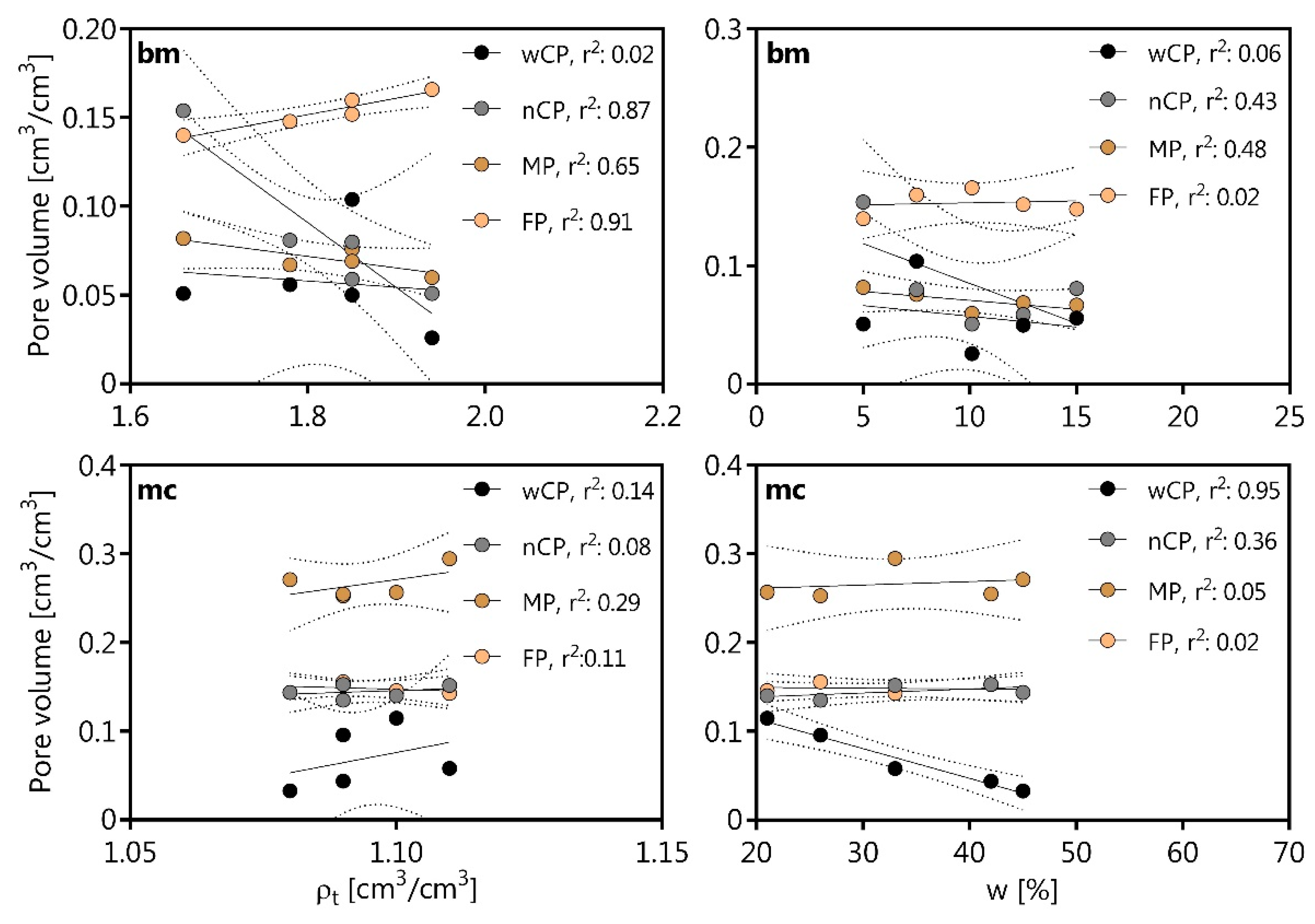
The linear regression analysis of the pore sizes of bm and mc with the bulk density (ρt) and the water content (w) during the Proctor test. Therefore, the nCP (r2: 0.87), MP (r2: 0.65), and FP (r2: 0.91) correlated positive to the ρt values of bm, while the wCP correlated positive to w (%) of mc with r2 of 0.95 (Figure 3).
3.3. Pore Size Distribution as Indicator of the Shrinkage-Dependent Volume Change
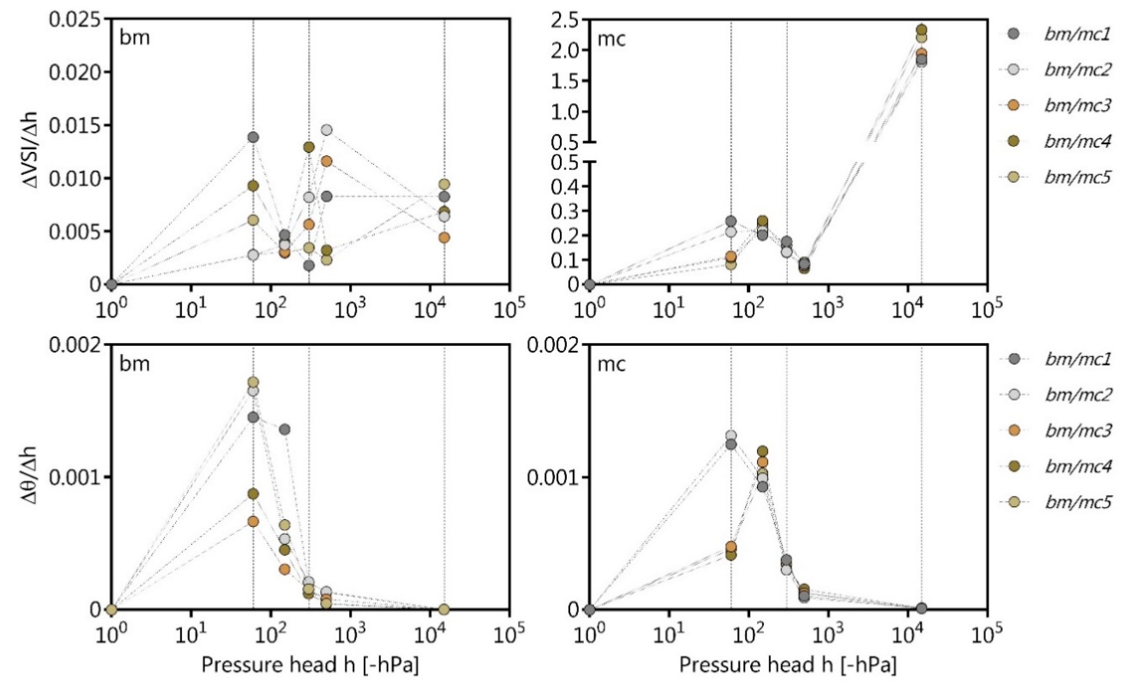
In general, the observed and pore size distribution correspondent shrinkage-induced volume change of bm was considerably lower than that of mc. The first structure peak is very distinct, and therefore the shrinkage-dependent volume change of bm1–bm5 (Figure 4), while the water loss between −60 and −300 hPa is not as significant for the volume change, except for bm1. The second matric peak and the corresponding volume change is more pronounced the higher the water loss within −300 and −15,000 hPa. For bm1, there is no significant volume change in the FP range (<−15,000 hPa), while the volume change of bm2−bm3 is less pronounced for the FP than for MP; the opposite trend has been observed for bm4−bm5 corresponding to the increased initial water content.
In case of mc1 and mc2, the emptying of the wCP (structural peak) results in a more pronounced water loss and thus shrinkage-dependent volume changes according to the PSD. Thus, the more pronounced the structural peak (−60 hPa), the higher the shrinkage-dependent volume change, especially for mc1−mc2. The emptying of the nCP and the first matric peak between −60 and −300 hPa lead also to an appropriate water loss resulting in a decrease in soil volume (Figure 4). The second matric peak between −300 and −15,000 hPa in the MP range indicates a less pronounced volume change, while the higher the amount of FP and initial water content (mc4−mc5), the more pronounced is the shrinkage-dependent volume change.
3.4. Compost and Its Function as Potential Soil Conditioner
The chemical properties of the compost used in this study are provided in Table 9. The dry substance content is 52 wt% with a pH value of 8.1, OC of 32 wt%, and ρs of 0.65 g/cm³; the content of total nitrogen is 1.2 wt%, phosphorus pentoxide 0.3 wt%, potassium oxide 0.6 wt%, magnesium oxide 0.4 wt%, and calcium oxide 2.2 wt% of the dry substance, respectively.
The sandy loam textured material is characterized by an alkaline character, while the OC content significantly increased from 1.0 to 4.6 wt% due to the compost application. The Ks values were higher and the ρt values of co were comparatively lower than of those of wco (Table 10). The AC and AWC values were significantly improved through compost application, while the Ks values of wco are up to 1 order of magnitude higher than of co.
The fitted θs values of co are comparatively higher than those of wco, and the LN and FX models predicted slightly higher θs values than the other models (Table 11).
The goodness of fit for the SWRC parameters obtained with bimodal and unimodal models are listed in Table 12. The bimodal models showed minimally higher coefficients of determination (r2 ≥ 0.99) than the unimodal models. The VG model fit and the BL model fit were found to be the best due to the more negative values of the AIC criterions as compared to all other models.
The RMSEθ values of the bimodal DB and BL models were comparatively lower than for the unimodal BC, VG, LN, and FX models. The smallest differences between fitted (xsim) and observed (xobs) θ values were found for the bimodal co with 0.008 cm3/cm3 (Table 13).
On the basis of the presented results, the authors decided to use the unimodal VG model and the bimodal BL model for further investigations of the pore size distribution (PSD).
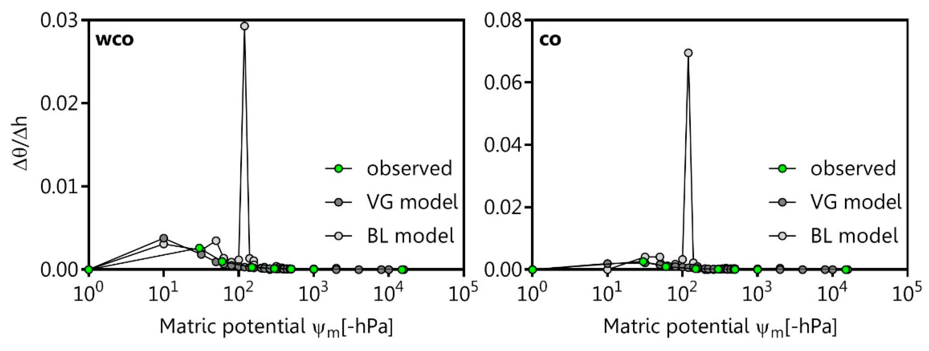
The observed and fitted PSD of wco and co are characterised by a mono-peak (structural peak) at approximately −100 hPa on the basis of the VG model and by a bi-peak structure with a first peak at −60 hPa and a second peak (porous matric peak) at approximately −100 hPa described by the BL model (Figure 5).
In result, the bi-peak structure of co is more pronounced than of wco and the SWRCs describe that an emptying of structural pores here denoted as wCP (>−60 hPa) and textural pores denoted as nCP (−60 to −300 hPa) leads to a pronounced water loss. There are also more pronounced differences between the observed data and the VG model than with the BL model (Table 14).
4. Discussion
4.1. Suitability of Marsh Clay and Boulder Marl as Mineral Liner
Several studies assumed that natural and artificial soil compaction strongly affects the pore size distribution, and therefore the soil water retention characteristics [26,27]. Thus, the suitability of both investigated materials can be approved or is rather limited due to the installation conditions (degree of compaction) in landfill capping systems.
The total porosity values of bm were less pronounced than those of mc and may be explained by the lower ρt values and a smaller number of narrow coarse pores and medium pores. Thus, the comparatively higher silt and clay content of mc is a key factor as pointed out following [6,28]. Furthermore, the required threshold value for air capacity of ≥0.08 cm3/cm3 was only reached by mc1 and mc2. So, the installation of bm and mc as recultivation liner (top liner) cannot guarantee a sufficient plant growth [29], resulting in a restricted transpiration potential [30].
Hydraulic stresses can lead to periodic dehydration of the top liner potentially resulting in capillary rise from the bottom liner and possibly in the formation of undesirable shrinkage cracks [6]. Thus, the protective effect of the top liner must be ensured by a sufficient water storage capacity. In this case, the required available water capacity for topsoil liner of at least 0.14 cm3/cm3 per meter [2] was only reached by mc, even though the more pronounced shrinkage potential of the more clayey mc should be considered as described in a previous study [31]. Therefore, both tested materials are less effective as top liner material, and material improvements are necessary (i.e., additional compaction, compost or biochar addition) as suggested previously [6,13].
The presented Ks values of both materials were comparatively higher than the legal-fixed value of 5 × 10⁻⁹ m/s. Additional compaction may help to reduce the Ks values [26,32], but it is well known that quartz sand particles build-up stable structures with ongoing compaction [14], so the required Ks values, especially for bm, can hardly be reached [33]. In this case, the addition of three-layer clay minerals (i.e., smectite, vermiculite) could decrease the Ks values, but at the expense of an increasing shrinkage potential [34].
In case of the tested mc, there are various other types of clay with high to medium plasticity containing a low share of coarse sand fraction ensuring Ks values lower than 1 × 10⁻⁹ m/s after compaction, even after perennial wetting and drying cycles as tested following reference [35]. These clays should be preferred in construction of landfill liner, but low initial water contents near Proctor optimum should be applied during construction to prevent increasing Ks values due to the high shrinkage potential [6,36].
4.2. Pore Size Distribution and Modality of the SWRC
In general, the pore size distribution of the investigated bm and mc and therefore the SWRC characteristics are mainly influenced by the texture (i.e., [37]), content and type of clay (i.e., [22]), and the degree of compaction [28,38]. Several other authors also assuming the cation exchange capacity [39], the organic carbon content [40], and the shrinkage and swelling behaviour (i.e., [41]), but this is not included in the current study. The letter is extensively described for bm and mc, even considering in situ field conditions following [6,15].
In detail, the compaction during the Proctor test results in a rearrangement of soil particles by hydraulic and mechanical stresses which is associated with changes in the pore size distribution and the soil water retention characteristics [42]. Thus, the degree of compaction and the initial moisture content during installation are important factors for a mineral liner [5]. Furthermore, mathematical models complete the observed data for a better understanding of the soil water characteristics and to describe the influence of the here outlined factors on the pore size distribution.
In this study, the VG and FX model gave a better fitting performance than the BC and LN model with very small differences in the fitted output. The bimodal models showed minimal higher coefficients of determination (r2 ≥ 0.99) and gave the best fit for the observed soil water retention curves compared to the Proctor stages. It should also be mentioned that the VG or BL model are limited in describing the air entry pressure or the discontinuity of SWRC near the saturation point [22,23], thus differences between the modelled and observed data has to be taken in account in the data analysis.
The structural PSD peak of both materials was more pronounced on the dry side of the Proctor curve or rather at the Proctor optimum, if existing and could be explained by a) increasing dry bulk densities resulting in a loss of structural pores (bm) and b) increasing water content resulting in a homogenization and therefore a rearrangement of particles. The result is a loss in structural pores for mc as previously described [42]. The wet side of the Proctor curve with higher water contents is characterized by a less pronounced structural peak, but a more pronounced matric peak, especially for mc4 and mc5, that corresponds to a higher water loss of textural pores. This circumstance also indicates a higher shrinkage tendency than for aggregated soils due to higher values of medium pores and fine pores for mc [27] as mentioned in reference [6]. The installation of mc in landfill capping systems may lead to a variety of conflicts (i.e., low permeability vs. high shrinkage tendency). Finally, soil compaction may reduce the volume of structural pores considerably, while most of the textural pores remain unaffected [41]. Even though several studies mentioned that the matric peak is strongly affected by the clay content and the structural PSD peak by the sand content (i.e., [22,23]), there was no significant textural effect in the investigated PSD curves.
4.3. Pore Size Distribution and Shrinkage Characteristics
In general, the proposed volume shrinkage index (VSI) of the investigated boulder marl (bm) and marsh clay (mc) can be characterized as a function of the pore size distribution that is also influenced by a) soil texture, b) clay content and type, c) initial water content, and d) degree of compaction [39,41]. In case of the mc, the PSD shows a similar trend like the volume shrinkage index (VSI) with changing pressure heads. Thus, the higher number of fine pores is obviously the main reason for the pronounced shrinkage-dependent volume change of textural pores in the range <−15,000 hPa, also mentioned by reference [34].
Otherwise, even the sand-dominated bm, where often pore rigidity is assumed, shows shrinkage-dependent volume change both in the structural and textural pores, but less pronounced than mc. Therefore, this assumption is disapproved regarding the study results. Nevertheless, the PSD-dependent and less distinct menisci forces and coinciding contraction of the soil particles during desiccation are the main reason for the limited volume change of sandy soils [16].
In summary, the pore size distribution is a good indicator for the shrinkage-dependent volume change more for the mc than for the bm, and further research is needed to develop pedotransfer functions which include the shrinkage behavior of differently textured soils as a function of the pore size distribution.
4.4. Compost Application
The investigated boulder marl (wco) of the Rastorf landfill is comparable with bm2 and bm3, thus, the application of compost significantly increased the amount of wide coarse pores, narrow coarse pores, medium pores, and fine pores and therefore the air capacity and available water capacity. It should also be noted that the available water capacity value of 0.122 cm3/cm3 for top liner is marginally lower than the statutory required of 0.14 cm3/cm3. As a result, the low AC and AWC values of wco can be compensated through compost application (co). However, the soil-compost mixture must at least ensure a sufficient water storage capacity to prevent a shrinkage-induced volume loss under field conditions [43]. It should also be taken in mind that the combination of temporally variable hydrophobic conditions [14,44], even during drier periods, and shrinkage cracks would lead to a more permeable, and thus, useless liner.
The soil-compost mixture as tested in the Rastorf landfill is an appropriate and cost-effective possibility to improve the quality of the top liner of landfill capping systems, even to ensure higher evapotranspiration rates [30] to decrease the undesired leachate generation. The results also indicate that the sand and silt content mainly influences the structural peak [23] and the significant water loss with ongoing dewatering of the narrow coarse pores (approximately −100 hPa) indicates also a volume change potential that should not be underestimated following references [37,41].
The application of biochar [13] or digestates [44] as soil conditioner should also be carefully tested under in situ field conditions, especially in the case of hydrophobic conditions and possible delayed rewetting after drier periods that potentially increase the risk of unintended shrinkage cracks.
5. Conclusions
This study was focused on the effect and improvement potential of soil compaction on the soil water retention curve characteristics or rather the pore size distribution of the differently-textured boulder marl and marsh clay. The used unimodal and bimodal models fitted the soil water retention curve reasonably well, but the bimodal DB and BL models enabled a better description of the soil water retention curve characteristics than the unimodal models.
The mono- or bi-modality of the observed and modelled pore size distributions, and thus the changes in the pore size distribution were found to be related to (i) the degree of compaction and (ii) the initial water content considering the different Proctor stages. The progress of the pore size distribution curve is also a promising indicator for the shrinkage-dependent volume change, although more research is needed with differently textured soils.
In conclusion, if considering the tested materials for a prospective use as a top and bottom liner material, especially a) the available water capacity must be improved (boulder marl) and b) the Ks values must be lowered (marsh clay). The former objective can be reached through compost application, while further investigations are needed to improve the material properties of the marsh clay.
Author Contributions
S.B.-B., H.H.G. and R.H. conceived the presented idea. S.B.-B. contributed the methodology, software, validation, visualization, and the formal analysis of the presented data. R.H. and H.H.G. supervised the findings of this study including conceptualization, supervision, and editing.
Funding
This research was funded by the Innovation Foundation of the federal state of Schleswig-Holstein and the ZMD Rastorf GmbH, Germany.
Conflicts of Interest
The funders had no role in the design of the study; in the collection, analyses, or interpretation of data; in the writing of the manuscript, or in the decision to publish the results.
References
- Laner, D.; Crest, M.; Schraff, H.; Morris, J.W.F.; Barlaz, M.A. A review of approaches for the long-term management of municipal solid waste landfills. Waste Manag. 2010, 32, 498–512. [Google Scholar] [CrossRef] [PubMed]
- German Landfill Ordinance. Deponieverordnung—DepV: Degree on Landfills (Ordinance to Simplify the Landfill Law)—Germany; In the form of the resolution of the Federal Cabinet dated 27 April 2009; Bundesministerium für Land-und Forstwirtschaft; Umwelt und Wasserwirtschaft: Bonn, Germany, 2009. [Google Scholar]
- Rowe, R.K. Systems engineering: The design and operation of municipal solid waste landfills to minimize contamination of groundwater. Geosynth. Int. 2011, 18, 391–404. [Google Scholar] [CrossRef]
- Pires, A.; Martinho, G.; Chang, N.B. Solid waste management in European countries: A review of system analysis techniques. J. Environ. Manag. 2011, 92, 1033–1050. [Google Scholar] [CrossRef] [PubMed]
- Beck-Broichsitter, S.; Fleige, H.; Horn, R. Waste capping systems processes and consequences for the longterm impermeability. In Soils within Cities; Levin, M., Kim, H.J., Morel, J.L., Burghardt, W., Charzynski, P., Shaw, R.K., Eds.; Catena Soil Sciences: Stuttgart, Germany, 2018; pp. 148–152. [Google Scholar]
- Beck-Broichsitter, S.; Gerke, H.H.; Horn, R. Suitability of Boulder Marl and Marsh Clay as Sealing Substrates for Landfill Capping Systems—A Practical Comparison. Geosciences 2018, 8, 356. [Google Scholar] [CrossRef]
- Anlauf, R.; Rehrmann, P. Effect of compaction on soil hydraulic parameters of vegetative landfill covers. Geomaterials 2012, 2, 29–36. [Google Scholar] [CrossRef]
- Proctor, R.R. Design and construction of rolled earth dams. Eng. News Rec. 1993, 111, 372–377. [Google Scholar]
- van Genuchten, M.T. A closed-form equation for predicting the hydraulic conductivity of unsaturated soils. Soil Sci. Soc. Am. J. 1980, 44, 892–898. [Google Scholar] [CrossRef]
- Seki, K. SWRC fit—A nonlinear fitting program with a water retention curve for soils having unimodal and bimodal pore structure. Hydrol. Earth Syst. Sci. Discuss. 2007, 4, 407–437. [Google Scholar] [CrossRef]
- Boden, A. Bodenkundliche Kartieranleitung, 5th ed.; German Soil Science Society: Hannover, Germany, 2005. [Google Scholar]
- Widomski, M.K.; Beck-Broichsitter, S.; Zink, A.; Fleige, H.; Horn, R. Numerical modeling of water balance for temporary landfill cover in North Germany. J. Plant Nutr. Soil Sci. 2015, 178, 401–412. [Google Scholar] [CrossRef]
- Ajayi, A.; Horn, R. Comparing the potentials of clay and biochar in improving water retention and mechanical resilience of sandy soil. Int. Agrophys. 2016, 30, 391–399. [Google Scholar] [CrossRef] [Green Version]
- Beck-Broichsitter, S.; Fleige, H.; Horn, R. Compost quality and its function as soil conditioner of recultivation layers—A critical review. Int. Agrophys. 2018, 32, 11–18. [Google Scholar] [CrossRef]
- Beck-Broichsitter, S.; Gerke, H.H.; Horn, R. Shrinkage characteristics of boulder marl as sustainable mineral liner material of landfill capping systems. Sustainability 2018, 10, 4025. [Google Scholar] [CrossRef]
- Hartge, K.H.; Horn, R. Essential Soil Physics—An Introduction to Soil Processes, Structure, and Mechanics; Horton, R., Horn, R., Bachmann, J., Peth, S., Eds.; Schweizerbart Science Publishers: Stuttgart, Germany, 2016. [Google Scholar]
- Hartge, K.H. Ein Haubenpermeameter zum schnellen Durchmessen zahlreicher Stechzylinderproben. Z. Kulturtech. Flurbereinigung 1966, 7, 155–163. [Google Scholar]
- Brooks, R.H.; Corey, A.T. Hydraulic Properties of Porous Media; Hydrol. Paper 3; Colorado State Univ.: Fort Collins, CO, USA, 1964. [Google Scholar]
- Fredlund, D.G.; Xing, A. Equations for the soil-water characteristic curve. Can. Geotech. J. 1994, 31, 521–532. [Google Scholar] [CrossRef]
- Kosugi, K. Lognormal distribution model for unsaturated soil hydraulic properties. Water Resour. Res. 1996, 32, 2697–2703. [Google Scholar] [CrossRef]
- Durner, W. Hydraulic conductivity estimation for soils with heterogeneous pore structure. Water Resour. Res. 1994, 26, 1483–1496. [Google Scholar] [CrossRef]
- Dexter, A.; Czyz, E.; Richard, G.; Reszkowska, A. A user-friendly water retention function that takes account of the textural and structural pore spaces in soil. Geoderma 2008, 143, 113–118. [Google Scholar] [CrossRef]
- Ding, D.; Zhao, Y.; Feng, H.; Peng, X.; Si, B. Using the double-exponential water retention equation to determine how soil pore-size distribution is linked to soil texture. Soil Tillage Res. 2016, 156, 119–130. [Google Scholar] [CrossRef]
- Hurvich, C.M.; Tsai, C.-L. Regression and time series model selection in small sample. Biometrika 1989, 76, 99–104. [Google Scholar] [CrossRef]
- Mazerolle, M.J. Improving data analysis in herpetology: Using Akaike’s Information Criterion (AIC) to assess the strength of biological hypotheses. Amphibia-Reptilia 2006, 27, 169–180. [Google Scholar] [CrossRef]
- Zhang, S.L.; Grip, H.; Lovdahl, L. Effect of soil compaction on hydraulic properties of two loess soils in China. Soil Tillage Res. 2006, 90, 117–125. [Google Scholar] [CrossRef]
- Horn, R.; Baumgartl, T. Dynamic Properties of Soils. In Soil Physics Companion; Warrick, A.W., Ed.; CRC Press LLC: Boca Raton, FL, USA, 2002; pp. 17–48. [Google Scholar]
- Schäffer, B.; Schulin, R.; Boivin, P. Changes in shrinkage of restored soil caused by compaction beneath heavy agricultural machinery. Eur. J. Soil Sci. 2008, 59, 771–783. [Google Scholar] [CrossRef]
- Hauser, V.L. Evapotranspiration Covers for Landfills and Waste Sites; CRC Press, Taylor & Francis: Boca Raton, FL, USA, 2008. [Google Scholar]
- Beck-Broichsitter, S.; Gerke, H.H.; Horn, R. Assessment of leachate production from a municipal solid waste landfill through water balance modelling. Geosciences 2018, 8, 372. [Google Scholar] [CrossRef]
- Markgraf, W.; Watts, C.W.; Whalley, W.R.; Hrkac, T.; Horn, R. Influence of organic matter on rheological properties of soil. Appl. Clay Sci. 2012, 64, 25–33. [Google Scholar] [CrossRef]
- Zink, A.; Fleige, H.; Horn, R. Load risks of subsoil compaction and depths of stress propagation in arable Luvisols. Soil Sci. Soc. Am. J. 2010, 74, 1733–1742. [Google Scholar] [CrossRef]
- Stępniewski, W.; Widomski, M.K.; Horn, R. Hydraulic conductivity and landfill construction. In Developments in Hydraulic Conductivity Research, Rijeka, Croatia, 2011; Dikinya, O., Ed.; Intech: Rijeka, Croatia, 2011; pp. 249–270. [Google Scholar]
- Costa, S.; Kodikara, J.; Shannon, B. Salient factors controlling desiccation cracking of clay in laboratory experiments. Géotechnique 2013, 63, 18–29. [Google Scholar] [CrossRef]
- Widomski, M.K.; Musz-Pomorska, A.; Stępniewski, W. Clays of different plasticity as materials for landfill liners in rural systems of sustainable waste management. Sustainability 2018, 10, 2489. [Google Scholar] [CrossRef]
- Widomski, M.K.; Stępniewski, W.; Horn, R.; Bieganowski, A.; Gazda, L.; Franus, M.; Pawlowski, M. Shrink-swell potential, hydraulic conductivity and geotechnical properties of clay materials for landfill liner construction. Int. Agrophys. 2015, 29, 365–375. [Google Scholar] [CrossRef] [Green Version]
- Gebhardt, S.; Fleige, H.; Horn, R. Anisotropic shrinkage of mineral and organic soils and its impact on soil hydraulic properties. Soil Tillage Res. 2012, 125, 96–104. [Google Scholar] [CrossRef]
- Horn, R.; Peng, X.; Fleige, H.; Dörner, J. Pore rigidy in structured soils—Only a theoretical boundary condition for hydraulic properties. J. Soil Sci. Plant Nutr. 2014, 60, 3–14. [Google Scholar]
- Dexter, A.; Richard, G.; Arrouays, D.; Czyz, E.; Jolivet, C.; Duval, O. Complexed organic matter controls soil physical properties. Geoderma 2008, 144, 620–627. [Google Scholar] [CrossRef]
- Leue, M.; Ellerbrock, R.H.; Gerke, H.H. DRIFT mapping of organic matter composition at intact soil aggregate surfaces. Vadose Zone J. 2010, 9, 317–324. [Google Scholar] [CrossRef]
- Peng, X.; Horn, R. Identifying six types of soil shrinkage curves from a large set of experimental data. Soil Sci. Soc. Am. J. 2013, 77, 372–381. [Google Scholar] [CrossRef]
- Alaoui, A.; Lipiec, J.; Gerke, H.H. A review of the changes in the soil pore system due to soil deformation: A hydrodynamic perspective. Soil Tillage Res. 2011, 115–116, 1–15. [Google Scholar] [CrossRef]
- Maylavarpu, R.S.; Zinati, G.M. Improvement of soil properties using compost for optimum parsley production in sandy soils. Sci. Horticult. 2009, 120, 131–140. [Google Scholar] [CrossRef]
- Voelkner, A.; Ohl, S.; Holthusen, D.; Hartung, E.; Dörner, J.; Horn, R. Impact of mechanically pre-treated anorganic digestates om soil properties. J. Soil Sci. Plant Nutr. 2015, 155, 882–895. [Google Scholar]
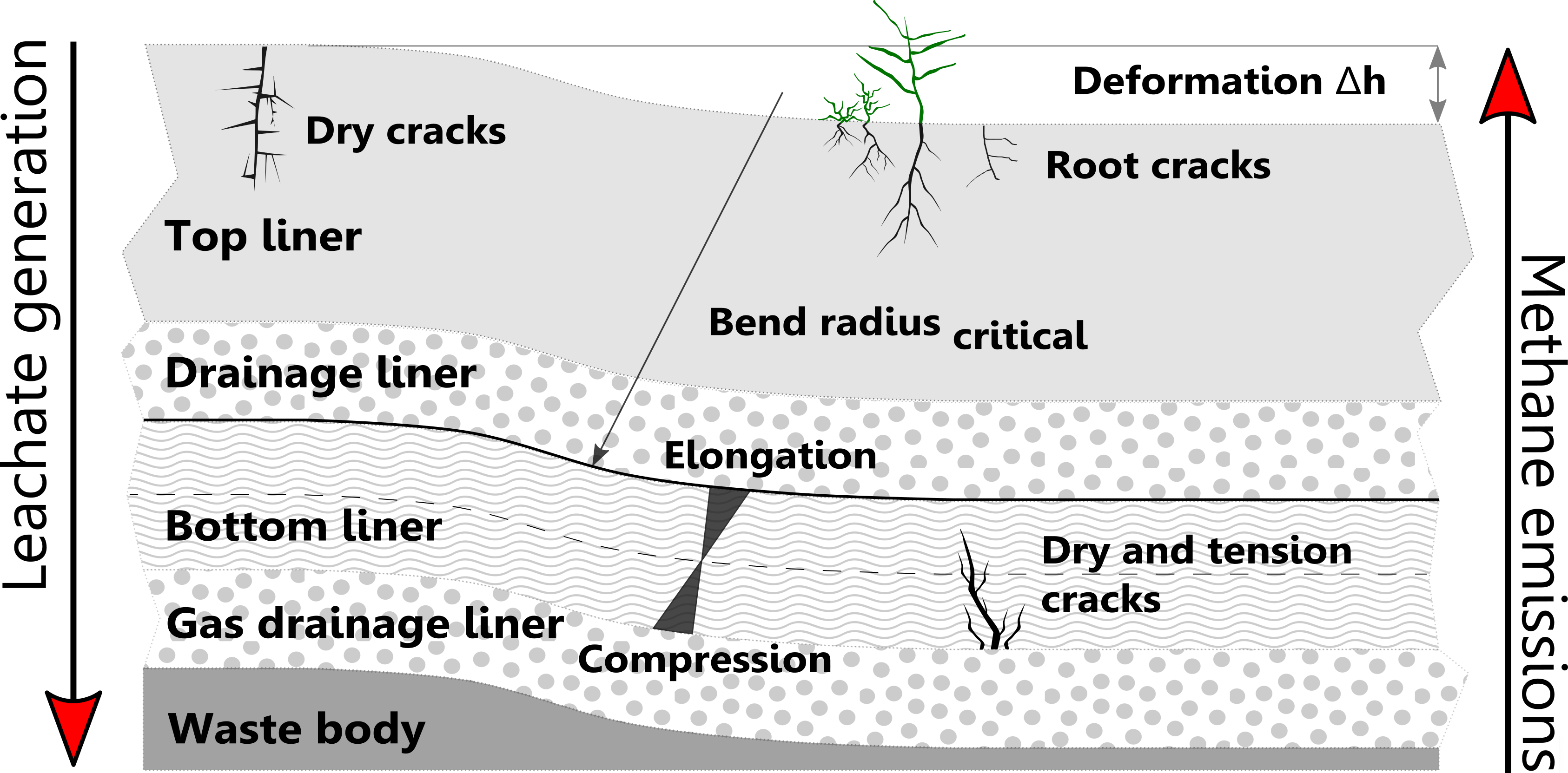
Figure 1.
Bi- and unimodal soil water retention curves of the boulder marl (bm) and marsh clay (mc) for five different Proctor stages (bm1–bm5, mc1–mc5) of the following models: BC model [18], VG model [9], FX model [19], LN model [20], DB model [21], and BL model [22].

Figure 2.
Fitted and observed pore size distribution as ratio of changing volumetric water content (θ) and pressure head (h) of the boulder marl (bm) and the marsh clay (mc) of five different Proctor stages (1–5) considering the VG model [9] and BL model [22].

Figure 3.
Linear regression of the pore volume fractions per size class for boulder marl (bm) and marsh clay (mc) with the dry bulk density (ρt) and the gravimetric water content (w) during the Proctor test. The pore sizes are classified as follows: wCP = wide coarse pores (>50 μm; >−60 hPa), nCP = narrow coarse pores (50–10 μm; −60 to −300 hPa), MP = medium pores (<10–2 μm; −300 to −15,000 hPa), FP = fine pores (<2 μm; <−15,000 hPa). The r2 indicates the coefficient of determination. The dashed lines indicate the confidence limits for a confidence level of 95%.

Figure 4.
Observed pore size distribution as ratio of changing volumetric water content (θ) and pressure head (h) and pore size distribution (PSD)-dependent volume change as ratio volume shrinkage index (VSI) and pressure head (h) of the boulder marl (bm) and the marsh clay (mc) of five different Proctor stages (1–5).

Figure 5.
Fitted and observed pore size distribution as ratio of changing volumetric water content (θ) and pressure head (h) of the boulder marl without compost (wco) and with compost (co) considering the VG model [9] and BL model [22].


Table 1.
Soil characteristics of boulder marl (bm) and marsh clay (mc) with 4 replicate measurements for organic carbon (OC), pH value, texture, and particle density (ρs), respectively. The symbol ± indicates the standard deviation. SL, CL = [11].
Table 1.
Soil characteristics of boulder marl (bm) and marsh clay (mc) with 4 replicate measurements for organic carbon (OC), pH value, texture, and particle density (ρs), respectively. The symbol ± indicates the standard deviation. SL, CL = [11].
| OC | pH | Sand | Silt | Clay | ρs | Texture | |
|---|---|---|---|---|---|---|---|
| [wt%] | [CaCl2] | [wt%] | [wt%] | [wt%] | [g/cm3] | [–] | |
| bm | 0.05 ± 0.02 | 7.6 ± 0.3 | 68 ± 1 | 21 ± 2 | 11 ± 2 | 2.65 ± 0.2 | SL |
| mc | 0.25 ± 0.03 | 5.6 ± 0.2 | 18 ± 1 | 56 ± 2 | 26 ± 3 | 2.67 ± 0.3 | CL |
Table 2.
Proctor density (ρPr) and moisture content (w) of the boulder marl (bm) and marsh clay (mc) with 10 soil cores per Proctor stage.
Table 2.
Proctor density (ρPr) and moisture content (w) of the boulder marl (bm) and marsh clay (mc) with 10 soil cores per Proctor stage.
| bm1 | bm2 | bm3 | bm4 | bm5 | mc1 | mc2 | mc3 | mc4 | mc5 | ||
|---|---|---|---|---|---|---|---|---|---|---|---|
| ρPr | [g/cm³] | 1.67 | 1.98 | 2.07 | 2.03 | 1.95 | 1.09 | 1.25 | 1.34 | 1.23 | 1.13 |
| w | [%] | 5.0 | 7.5 | 10.1 | 12.5 | 15.0 | 21 | 26 | 33 | 42 | 45 |
Table 3.
Soil physical properties of the investigated boulder marl (bm1–bm5) and marsh clay (mc1–mc5) considering the dry bulk density (ρt), air capacity (AC), the plant available water capacity (AWC), and saturated hydraulic conductivity (Ks) with 10 to 15 soil cores per Proctor stage. The symbol ± indicates the standard deviation.
| ρt | AC | AWC | Ks | ρt | AC | AWC | Ks | ||
|---|---|---|---|---|---|---|---|---|---|
| [g/cm3] | [cm3/cm3] | [cm3/cm3] | [m/s] | [g/cm3] | [cm3/cm3] | [cm3/cm3] | [m/s] | ||
| bm1 | 1.66 | 0.051 | 0.081 | 1.6 × 10⁶ | mc1 | 1.10 | 0.115 | 0.256 | 7.4 × 10⁷ |
| bm2 | 1.85 | 0.054 | 0.076 | 1.8 × 10⁶ | mc2 | 1.09 | 0.096 | 0.253 | 3.2 × 10⁷ |
| bm3 | 1.94 | 0.026 | 0.059 | 1.2 × 10⁶ | mc3 | 1.11 | 0.582 | 0.244 | 1.2 × 10⁷ |
| bm4 | 1.85 | 0.049 | 0.069 | 7.8 × 10⁷ | mc4 | 1.09 | 0.043 | 0.255 | 3.8 × 10⁷ |
| bm5 | 1.78 | 0.056 | 0.067 | 3.8 × 10⁷ | mc5 | 1.08 | 0.033 | 0.271 | 6.8 × 10⁷ |
Table 4.
Fitted soil water retention curve parameters of the boulder marl (bm): Brooks–Corey (BC) model [18], van Genuchten (VG) model [9], Fredlund and Xing (FX) model [19], Kosugi (LN) model [20], Durner (DB) model [21], and Seki (BL) model [10].
| BC | θs | θr | hb | λ | LN | θs | θr | h | σ | |
| [cm3/cm3] | [cm] | [–] | [cm3/cm3] | [cm] | [–] | |||||
| bm1 | 0.422 | 0.135 | 45.61 | 0.687 | bm1 | 0.434 | 0.152 | 127.7 | 1.085 | |
| bm2 | 0.420 | 0.134 | 17.42 | 0.371 | bm2 | 0.423 | 0.162 | 102.4 | 1.812 | |
| bm3 | 0.299 | 0.139 | 38.05 | 0.309 | bm3 | 0.304 | 0.166 | 230.8 | 1.587 | |
| bm4 | 0.329 | 0.107 | 19.33 | 0.242 | bm4 | 0.333 | 0.151 | 179.5 | 2.026 | |
| bm5 | 0.353 | 0.131 | 28.61 | 0.409 | bm5 | 0.360 | 0.155 | 140.7 | 1.475 | |
| VG | θs | θr | α | n | FX | θs | θr | α | n | m |
| [cm3/cm3] | [1/cm] | [–] | [cm3/cm3] | [1/cm] | [–] | [–] | ||||
| bm1 | 0.433 | 0.145 | 0.014 | 2.007 | bm1 | 0.425 | 5 x 10⁻⁵ | 54.94 | 0.367 | 3.891 |
| bm2 | 0.421 | 0.147 | 0.034 | 1.495 | bm2 | 0.421 | 0.099 | 33.23 | 0.815 | 1.276 |
| bm3 | 0.303 | 0.156 | 0.014 | 1.522 | bm3 | 0.303 | 0.092 | 65.03 | 0.499 | 1.530 |
| bm4 | 0.332 | 0.130 | 0.028 | 1.360 | bm4 | 0.331 | 2 × 10⁻⁶ | 33.87 | 0.366 | 1.325 |
| bm5 | 0.359 | 0.114 | 0.019 | 1.643 | bm5 | 0.357 | 9 × 10⁻⁸ | 40.26 | 0.307 | 2.676 |
| DB | θs | θr | w1 | α1 | n1 | α2 | n2 | |||
| [cm3/cm3] | [–] | [1/cm] | [–] | [1/cm] | [–] | |||||
| bm1 | 0.424 | 0.139 | 0.660 | 0.014 | 3.893 | 0.002 | 2.455 | |||
| bm2 | 0.420 | 0.152 | 0.240 | 0.036 | 6.680 | 0.014 | 1.598 | |||
| bm3 | 0.303 | 0.157 | 0.079 | 0.017 | 4.998 | 0.010 | 1.559 | |||
| bm4 | 0.330 | 0.100 | 0.888 | 0.033 | 1.223 | 0.016 | 2.197 | |||
| bm5 | 0.353 | 0.142 | 0.497 | 0.018 | 4.643 | 0.004 | 1.726 | |||
| BL | θs | θr | w1 | hm1 | σ1 | hm2 | σ2 | |||
| [cm3/cm3] | [1/cm] | [1/cm] | [–] | [1/cm] | [–] | |||||
| bm1 | 0.423 | 0.139 | 0.617 | 78.26 | 0.451 | 523.8 | 0.881 | |||
| bm2 | 0.421 | 0.159 | 0.092 | 56.63 | 0.060 | 120.6 | 1.926 | |||
| bm3 | 0.302 | 0.165 | 0.127 | 59.47 | 0.050 | 309.9 | 1.532 | |||
| bm4 | 0.331 | 0.142 | 0.185 | 64.26 | 0.302 | 336.1 | 2.438 | |||
| bm5 | 0.353 | 0.147 | 0.428 | 58.81 | 0.303 | 448.2 | 1.457 | |||
Table 5.
Fitted soil water retention curve parameters of the marsh clay (mc): BC model [18], VG model [9], FX model [19], LN model [20], DB model [21], and BL model [22].
| BC | θs | θr | hb | λ | LN | θs | θr | h | σ | |
| [cm3/cm3] | [cm] | [–] | [cm3/cm3] | [cm] | [–] | |||||
| mc1 | 0.651 | 9 × 10⁻⁷ | 21.72 | 0.195 | mc1 | 0.663 | 0.103 | 402.5 | 2.516 | |
| mc2 | 0.635 | 0.001 | 23.65 | 0.181 | mc2 | 0.649 | 0.105 | 499.2 | 2.602 | |
| mc3 | 0.636 | 1 × 10⁻⁶ | 41.01 | 0.205 | mc3 | 0.652 | 0.101 | 617.6 | 2.225 | |
| mc4 | 0.590 | 0.001 | 44.77 | 0.194 | mc4 | 0.612 | 0.127 | 520.04 | 2.132 | |
| mc5 | 0.579 | 0.001 | 60.48 | 0.222 | mc5 | 0.598 | 0.123 | 587.4 | 1.923 | |
| VG | θs | θr | α | n | FX | θs | θr | α | m | n |
| [cm3/cm3] | [1/cm] | [–] | [cm3/cm3] | [1/cm] | [–] | [–] | ||||
| mc1 | 0.655 | 6 × 10⁻⁶ | 0.033 | 1.211 | mc1 | 0.671 | 3 × 10⁻⁷ | 161.3 | 1.359 | 0.648 |
| mc2 | 0.631 | 7 × 10⁻³ | 0.021 | 1.215 | mc2 | 0.656 | 6 × 10⁻³ | 181.5 | 1.305 | 0.631 |
| mc3 | 0.639 | 0.001 | 0.012 | 1.251 | mc3 | 0.657 | 0.001 | 267.04 | 1.321 | 0.751 |
| mc4 | 0.604 | 0.001 | 0.013 | 1.252 | mc4 | 0.615 | 0.001 | 165.35 | 0.988 | 0.852 |
| mc5 | 0.594 | 1 × 10⁻³ | 0.009 | 1.277 | mc5 | 0.601 | 0.004 | 220.08 | 1.031 | 0.917 |
| DB | θs | θr | w1 | α1 | n1 | α2 | n2 | |||
| [cm3/cm3] | [–] | [1/cm] | [–] | [1/cm] | [–] | |||||
| mc1 | 0.656 | 3 × 10⁻⁶ | 0.047 | 0.039 | 44.27 | 0.016 | 1.258 | |||
| mc2 | 0.640 | 9 × 10⁻⁶ | 0.038 | 0.045 | 3.79 | 0.016 | 1.233 | |||
| mc3 | 0.647 | 3 × 10⁻⁵ | 0.081 | 0.034 | 1.72 | 0.008 | 1.263 | |||
| mc4 | 0.604 | 0.002 | 0.022 | 0.012 | 37.85 | 0.012 | 1.251 | |||
| mc5 | 0.587 | 0.14 | 0.467 | 0.011 | 2.502 | 0.001 | 3.991 | |||
| BL | θs | θr | w1 | hm1 | σ1 | hm2 | σ2 | |||
| [cm3/cm3] | [1/cm] | [1/cm] | [–] | [1/cm] | [–] | |||||
| mc1 | 0.657 | 0.145 | 0.644 | 101.3 | 1.561 | 1060 | 0.105 | |||
| mc2 | 0.691 | 0.062 | 0.107 | 0.003 | 50.01 | 558.3 | 2.769 | |||
| mc3 | 0.722 | 0.007 | 0.779 | 625.9 | 2.278 | 309.9 | 2.721 | |||
| mc4 | 0.604 | 0.096 | 0.061 | 97.91 | 0.067 | 890.5 | 2.381 | |||
| mc5 | 0.586 | 0.144 | 0.428 | 119.9 | 0.709 | 1240 | 0.541 | |||
Table 6.
Coefficients of determination (r2) and AIC criterions (AICc) of the boulder marl (bm) and the marsh clay (mc): BC model [18], VG model [9], FX model [19], LN model [20], DB model [21], and BL model [22].
| BC | LN | VG | FX | DB | BL | |||||||
|---|---|---|---|---|---|---|---|---|---|---|---|---|
| r2 | AICc | r2 | AICc | r2 | AICc | r2 | AICc | r2 | AICc | r2 | AICc | |
| [–] | [–] | [–] | [–] | [–] | [–] | [–] | [–] | [–] | [–] | [–] | [–] | |
| bm1 | 0.997 | −76 | 0.982 | −67 | 0.993 | −62 | 0.997 | −75 | 0.999 | −99 | 0.999 | −92 |
| bm2 | 0.998 | −82 | 0.997 | −85 | 0.998 | −78 | 0.998 | −82 | 0.999 | −86 | 0.999 | −84 |
| bm3 | 0.996 | −86 | 0.997 | −95 | 0.998 | −88 | 0.998 | −93 | 0.999 | −99 | 0.999 | −94 |
| bm4 | 0.998 | −89 | 0.997 | −84 | 0.992 | −76 | 0.997 | −82 | 0.999 | −91 | 0.999 | −94 |
| bm5 | 0.998 | −85 | 0.979 | −70 | 0.988 | −65 | 0.995 | −75 | 0.993 | −86 | 0.999 | −88 |
| mc1 | 0.981 | −53 | 0.991 | −59 | 0.997 | −69 | 0.997 | −66 | 0.999 | −61 | 0.999 | −75 |
| mc2 | 0.981 | 18 | 0.991 | 12 | 0.994 | 8 | 0.994 | 11 | 0.994 | 15 | 0.994 | 15 |
| mc3 | 0.981 | 21 | 0.991 | 13 | 0.994 | 9 | 0.994 | 12 | 0.992 | 18 | 0.994 | 17 |
| mc4 | 0.986 | 15 | 0.993 | 10 | 0.991 | 13 | 0.991 | 15 | 0.994 | 14 | 0.996 | 12 |
| mc5 | 0.986 | 15 | 0.995 | 7 | 0.994 | 8 | 0.993 | 9 | 0.993 | 12 | 0.999 | −1 |
Table 7.
Root mean square error of the fitted water content (RMSEθ) of the boulder marl (bm) and marsh clay (mc): BC model [18], VG model [9], FX model [19], LN model [20], DB model [21], and BL model [22].
| BC | LN | VG | FX | DB | BL | |
|---|---|---|---|---|---|---|
| RMSEθ | ||||||
| [cm3/cm3] | ||||||
| bm1 | 0.006 | 0.009 | 0.012 | 0.006 | 0.003 | 0.003 |
| bm2 | 0.004 | 0.006 | 0.009 | 0.007 | 0.008 | 0.008 |
| bm3 | 0.003 | 0.002 | 0.002 | 0.002 | 0.002 | 0.002 |
| bm4 | 0.002 | 0.004 | 0.006 | 0.004 | 0.004 | 0.004 |
| bm5 | 0.003 | 0.002 | 0.009 | 0.004 | 0.002 | 0.002 |
| mc1 | 0.021 | 0.018 | 0.014 | 0.015 | 0.009 | 0.009 |
| mc2 | 0.019 | 0.014 | 0.014 | 0.014 | 0.014 | 0.014 |
| mc3 | 0.024 | 0.014 | 0.012 | 0.012 | 0.011 | 0.011 |
| mc4 | 0.016 | 0.013 | 0.011 | 0.011 | 0.009 | 0.009 |
| mc5 | 0.015 | 0.010 | 0.010 | 0.010 | 0.005 | 0.005 |
Table 8.
Bimodal and observed pore size distribution of the boulder marl (bm) and the marsh clay (mc) considering the unimodal VG model [9] and the bimodal BL model [10]. The pores sizes are classified as follows: wCP = wide coarse pores (>50 μm; >−60 hPa), nCP = narrow coarse pores (50–10 μm; −60 to −300 hPa), MP = medium pores (<10–2 μm; −300 to −15,000 hPa), FP = fine pores (<2 μm; <−15,000 hPa).
| Observed | VG Model | BL Model | ||||||||||
|---|---|---|---|---|---|---|---|---|---|---|---|---|
| wCP | nCP | MP | FP | wCP | nCP | MP | FP | wCP | nCP | MP | FP | |
| [cm3/cm3] | ||||||||||||
| bm1 | 0.051 | 0.154 | 0.082 | 0.140 | 0.065 | 0.155 | 0.066 | 0.146 | 0.050 | 0.154 | 0.080 | 0.140 |
| bm2 | 0.104 | 0.080 | 0.076 | 0.160 | 0.099 | 0.088 | 0.072 | 0.160 | 0.104 | 0.081 | 0.074 | 0.161 |
| bm3 | 0.026 | 0.051 | 0.060 | 0.166 | 0.025 | 0.053 | 0.058 | 0.166 | 0.027 | 0.049 | 0.060 | 0.166 |
| bm4 | 0.050 | 0.059 | 0.069 | 0.152 | 0.051 | 0.058 | 0.068 | 0.153 | 0.050 | 0.058 | 0.071 | 0.152 |
| bm5 | 0.056 | 0.081 | 0.067 | 0.148 | 0.066 | 0.011 | 0.072 | 0.121 | 0.056 | 0.078 | 0.071 | 0.148 |
| mc1 | 0.115 | 0.140 | 0.257 | 0.146 | 0.121 | 0.133 | 0.222 | 0.176 | 0.121 | 0.128 | 0.262 | 0.146 |
| mc2 | 0.096 | 0.135 | 0.253 | 0.156 | 0.087 | 0.126 | 0.233 | 0.182 | 0.114 | 0.114 | 0.267 | 0.154 |
| mc3 | 0.058 | 0.152 | 0.295 | 0.143 | 0.062 | 0.133 | 0.274 | 0.169 | 0.083 | 0.124 | 0.304 | 0.132 |
| mc4 | 0.044 | 0.153 | 0.255 | 0.153 | 0.062 | 0.126 | 0.254 | 0.161 | 0.060 | 0.124 | 0.266 | 0.153 |
| mc5 | 0.033 | 0.144 | 0.271 | 0.144 | 0.049 | 0.123 | 0.272 | 0.149 | 0.031 | 0.141 | 0.271 | 0.144 |
Table 9.
Average dry substance content (DS), pH value, nutrient and organic carbon (OC), and particle density (ρs) of the compost made out of trees and shrubs (Rastorf, Northern Germany).
Table 9.
Average dry substance content (DS), pH value, nutrient and organic carbon (OC), and particle density (ρs) of the compost made out of trees and shrubs (Rastorf, Northern Germany).
| DS | pH | OC | Nt | P2O5 | K2O | MgO | CaO | ρs | |
|---|---|---|---|---|---|---|---|---|---|
| [wt%] | [CaCl2] | [wt%] | [wt%] | [wt%] | [wt%] | [wt%] | [wt%] | [g/cm3] | |
| compost | 52 | 8.1 | 32 | 1.2 | 0.3 | 0.6 | 0.4 | 2.2 | 0.65 |
Table 10.
Soil characteristics of boulder marl without compost (wco) and with compost (co), with 4 replicate measurements for organic carbon (OC), pH value, texture, particle density (ρs), respectively. Dry bulk density (ρt), air capacity (AC), the plant available water capacity (AWC), and saturated hydraulic conductivity (Ks) with 10 to 15 soil cores, respectively. The symbol ± indicates the standard deviation.
| OC | pH | Sand | Silt | Clay | ρs | ρt | AC | AWC | Ks | |
|---|---|---|---|---|---|---|---|---|---|---|
| [wt%] | [CaCl2] | [wt%] | [wt%] | [wt%] | [g/cm3] | [g/cm3] | [cm3/cm3] | [cm3/cm3] | [m/s] | |
| wco | 1.0 | 7.6 ± 0.2 | 77 ± 2 | 13 ± 1 | 10 ± 1 | 2.63 | 1.77 | 0.105 | 0.084 | 7.1 × 10⁶ |
| co | 4.6 | 7.4 ± 0.1 | 80 ± 1 | 13 ± 2 | 7 ± 2 | 2.36 | 1.13 | 0.121 | 0.122 | 2.7 × 10⁵ |
Table 11.
Fitted soil water retention curve parameters of the boulder marl without compost (wco) and with compost (co): BC model [18], VG model [9], FX model [19], LN model [20], DB model [21], and BL model [22].
| BC | θs | θr | hb | λ | LN | θs | θr | h | σ | |
| [cm3/cm3] | [cm] | [–] | [cm3/cm3] | [cm] | [–] | |||||
| wco | 0.312 | 0.001 | 6.751 | 0.183 | wco | 0.313 | 0.066 | 118.1 | 2.849 | |
| co | 0.442 | 0.041 | 15.93 | 0.267 | co | 0.451 | 0.109 | 144.1 | 1.898 | |
| VG | θs | θr | α | n | FX | θs | θr | α | n | m |
| [cm3/cm3] | [1/cm] | [–] | [cm3/cm3] | [1/cm] | [–] | [–] | ||||
| wco | 0.312 | 0.008 | 0.117 | 1.201 | wco | 0.312 | 0.058 | 179.7 | 0.507 | 2.856 |
| co | 0.439 | 0.077 | 0.031 | 1.397 | co | 0.451 | 0.114 | 2833 | 0.623 | 13.10 |
| DB | θs | θr | w1 | α1 | n1 | α2 | n2 | |||
| [cm3/cm3] | [–] | [1/cm] | [–] | [1/cm] | [–] | |||||
| wco | 0.312 | 0.074 | 0.640 | 0.071 | 1.774 | 0.002 | 2.091 | |||
| co | 0.442 | 0.117 | 0.391 | 0.038 | 4.147 | 0.003 | 2.351 | |||
| BL | θs | θr | w1 | hm1 | σ1 | hm2 | σ2 | |||
| [cm3/cm3] | [1/cm] | [1/cm] | [–] | [1/cm] | [–] | |||||
| wco | 0.312 | 0.077 | 0.555 | 23.86 | 1.098 | 703.5 | 1.045 | |||
| co | 0.441 | 0.118 | 0.351 | 29.16 | 0.112 | 340.7 | 0.958 | |||
Table 12.
Coefficients of determination (r2) and AIC criterions (AICc) of the boulder marl without compost (wco) and with compost (co): BC model [18], VG model [9], FX model [19], LN model [20], DB model [21], and BL model [22].
| BC | LN | VG | FX | DB | BL | |||||||
|---|---|---|---|---|---|---|---|---|---|---|---|---|
| r2 | AICc | r2 | AICc | r2 | AICc | r2 | AICc | r2 | AICc | r2 | AICc | |
| [–] | [–] | [–] | [–] | [–] | [–] | [–] | [–] | [–] | [–] | [–] | [–] | |
| wco | 0.996 | −79 | 0.996 | −80 | 0.997 | −83 | 0.997 | −81 | 0.997 | −108 | 0.997 | −110 |
| co | 0.978 | −59 | 0.983 | −65 | 0.993 | −61 | 0.991 | −66 | 0.999 | −79 | 0.998 | −75 |
Table 13.
Root mean square error of the fitted water content (RMSEθ) of the boulder marl without compost (wco) and with compost (co): BC model [18], VG model [9], FX model [19], LN model [20], DB model [21], and BL model [22].
| BC | LN | VG | FX | DB | BL | |
|---|---|---|---|---|---|---|
| RMSEθ | ||||||
| [cm3/cm3] | ||||||
| wco | 0.011 | 0.014 | 0.017 | 0.018 | 0.010 | 0.010 |
| co | 0.016 | 0.016 | 0.013 | 0.015 | 0.008 | 0.008 |
Table 14.
Bimodal and observed pore size distribution of the boulder marl without compost (wco) and with compost (co) considering the unimodal VG model [9] and the bimodal BL model [22]. The pores sizes are classified as follows: wCP = wide coarse pores (>50 μm; >−60 hPa), nCP = narrow coarse pores (50–10 μm; −60 to −300 hPa), MP = medium pores (<10–2 μm; −300 to −15,000 hPa), FP = fine pores (<2 μm; <−15,000 hPa).
| Observed | VG Model | BL Model | ||||||||||
|---|---|---|---|---|---|---|---|---|---|---|---|---|
| wCP | nCP | MP | FP | wCP | nCP | MP | FP | wCP | nCP | MP | FP | |
| [cm3/cm3] | ||||||||||||
| wco | 0.105 | 0.046 | 0.083 | 0.077 | 0.098 | 0.054 | 0.081 | 0.075 | 0.105 | 0.045 | 0.084 | 0.077 |
| co | 0.121 | 0.081 | 0.122 | 0.116 | 0.107 | 0.108 | 0.115 | 0.108 | 0.121 | 0.086 | 0.116 | 0.118 |
© 2018 by the authors. Licensee MDPI, Basel, Switzerland. This article is an open access article distributed under the terms and conditions of the Creative Commons Attribution (CC BY) license (http://creativecommons.org/licenses/by/4.0/).
Share and Cite
MDPI and ACS Style
Beck-Broichsitter, S.; Gerke, H.H.; Horn, R. Effect of Compaction on Soil Physical Properties of Differently Textured Landfill Liner Materials. Geosciences 2019, 9, 1. https://doi.org/10.3390/geosciences9010001
AMA Style
Beck-Broichsitter S, Gerke HH, Horn R. Effect of Compaction on Soil Physical Properties of Differently Textured Landfill Liner Materials. Geosciences. 2019; 9(1):1. https://doi.org/10.3390/geosciences9010001
Chicago/Turabian StyleBeck-Broichsitter, Steffen, Horst H. Gerke, and Rainer Horn. 2019. "Effect of Compaction on Soil Physical Properties of Differently Textured Landfill Liner Materials" Geosciences 9, no. 1: 1. https://doi.org/10.3390/geosciences9010001
Note that from the first issue of 2016, this journal uses article numbers instead of page numbers. See further details here.