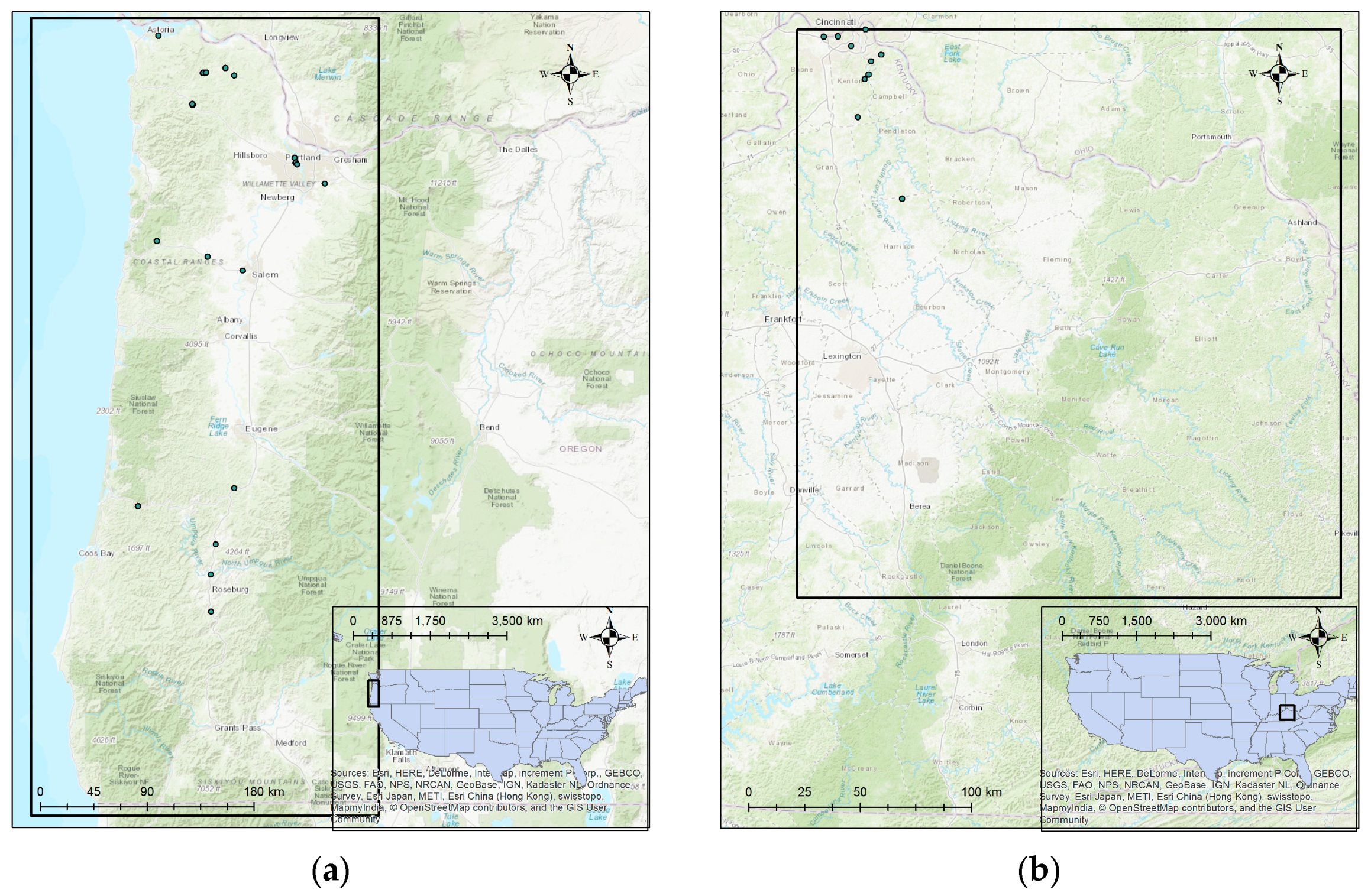
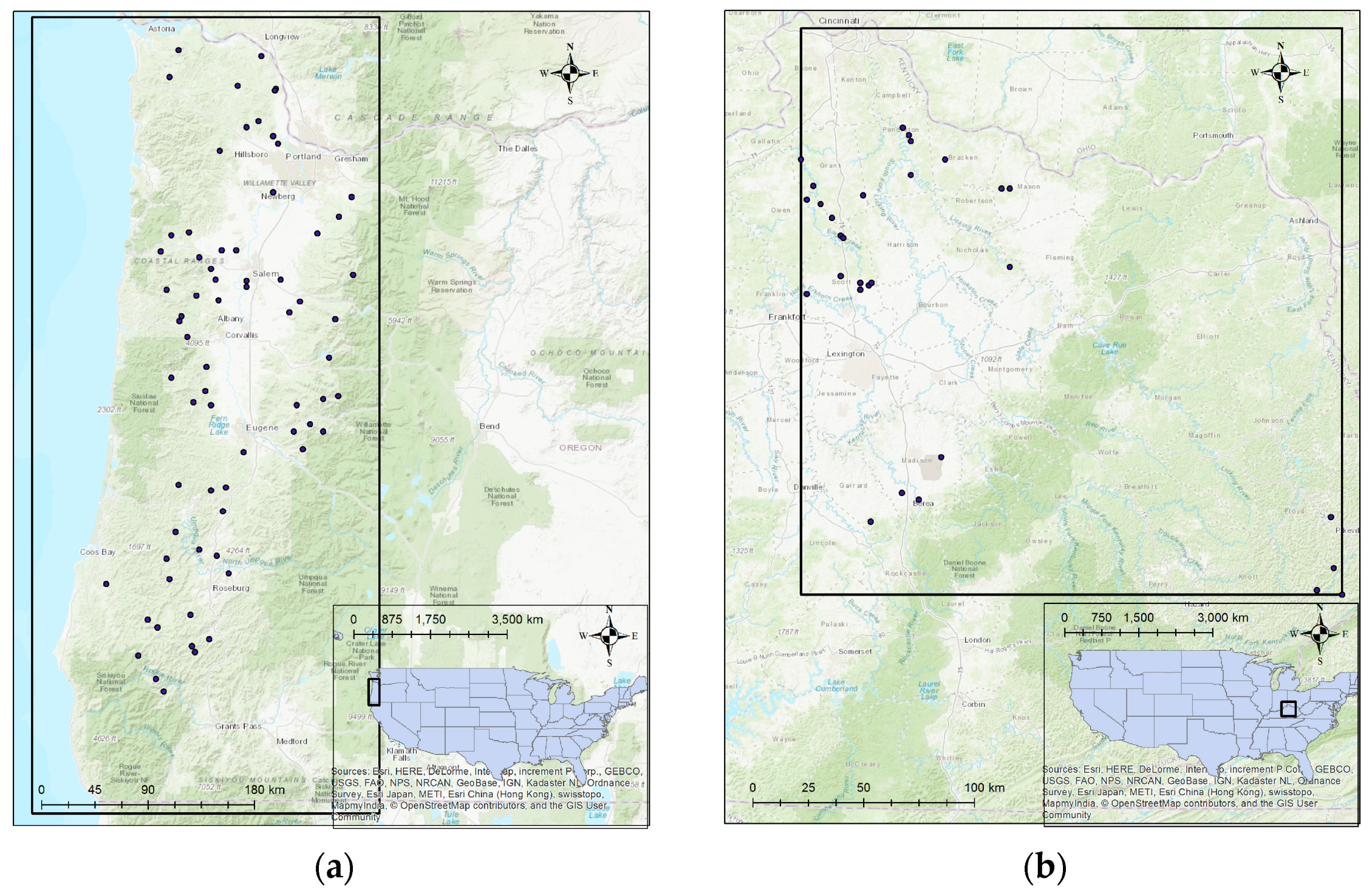
Article

An Improved Data-Driven Approach for the Prediction of Rainfall-Triggered Soil Slides Using Downscaled Remotely Sensed Soil Moisture

by
Thilanki Dahigamuwa
1,*,
Manjriker Gunaratne
1 and
Mingyang Li
2
1
Department of Civil and Environmental Engineering, University of South Florida, Tampa, FL 33620, USA
2
Department of Industrial and Management Systems Engineering, University of South Florida, Tampa, FL 33620, USA
*
Author to whom correspondence should be addressed.
Geosciences 2018, 8(9), 326; https://doi.org/10.3390/geosciences8090326
Submission received: 6 June 2018 / Revised: 3 August 2018 / Accepted: 18 August 2018 / Published: 30 August 2018
(This article belongs to the Section Natural Hazards)

Abstract

:
The infiltration of rainwater into soil slopes leads to an increase of porewater pressure and destruction of matric suction, which causes a reduction in soil shear strength and slope instability. Hence, surface moisture and infiltration properties must be direct inputs in reliable landslide hazard assessment methods. Since the in situ measurement of pore pressure is expensive, the use of remotely sensed soil moisture is practically feasible. Downscaling improves the spatial resolution of soil moisture for a better representation of specific local conditions. Downscaled soil moisture, the relevant geotechnical properties of saturated hydraulic conductivity and soil type, and the conditioning factors of elevation, slope, and distance to roads are used to develop an improved logistic regression model to predict the soil slide hazard of soil slopes using data from two geographically different regions. A soil moisture downscaling model with a better accuracy than the downscaling models that have been used in previous landslide studies is employed in this study. This model provides a good classification accuracy and performs better than the alternative water drainage-based indices that are conventionally used to quantify the effect that elevated soil moisture has upon the soil slide hazard. Furthermore, the downscaling of soil moisture content is shown to improve the prediction accuracy. Finally, a technique that can provide the threshold probability for identifying locations with a high soil slide hazard is proposed.

1. Introduction

The objective of this study is to present a framework for using remotely sensed soil moisture available on a daily basis to monitor locations that are highly susceptible to rainfall-triggered soil slides, with a well-structured assessment procedure. Furthermore, the performance of downscaled remotely sensed soil moisture in soil slide hazard assessment is compared with that of widely used water-drainage based variables, namely distance to drainage, drainage density, and the Topographic Wetness Index (TWI). Moreover, an improved approach for identifying a threshold for classifying soil slide and non-soil slide locations is proposed.

1.1. Background of the Study

Soil slides present a major threat to humans and cause widespread damage to property and lives throughout the world. The stability of a naturally existing soil slope is achieved through the balance of forces acting upon it. Slope instability and subsequent sliding occur due to the action of a trigger, which can disrupt this balance. Triggering factors such as rainfall, seismic activity, volcanic eruptions, or wildfire can cause soil slides [1]. Of these triggering factors, rainfall is the most common triggering factor [1,2,3,4]; hence, this research focuses on rainfall-triggered soil slides.
Rainfall-triggered soil slides commonly occur in regions consisting of residual soil slopes that are naturally stabilized by negative pore water pressure or matric suction. With the infiltration of rainwater, the soil moisture content increases, thereby destructing the matric suction. This phenomenon results in a decreased effective stress and hence, soil shear strength and increased weight of soil, causing slope instability [3]. Thus, it is realized that if the site soil moisture content can be used directly as a predictor in assessing soil slide hazards, the accuracy of predicting rainfall-triggered soil slides can be improved. Past researchers have attempted to use in situ soil moisture measurements as a tool for soil slide hazard assessment [4,5,6]. However, measuring in situ soil moisture can be a prohibitive task due to the extensive instrumentation requirements and unreliability of instrument readings. Thus, the use of remotely sensed soil moisture has been suggested as an alternative to in situ soil moisture measurements [7,8,9]. It is believed that soil moisture records that are acquired form satellites on a regular basis would be particularly effective in such assessments.
On the other hand, most current soil slide prediction methods use indirect means of evaluating the increases in moisture such as the use of hydrological conditioning factors (Section 1.2), including distance to drainage, drainage density, and the Topographic Wetness Index or other similar water-drainage based variables [4,10,11]. The distance to drainage accessories affects the drainage of rainwater from a basin. A higher distance to drainage accessories (streams or water bodies) would indicate a slower drainage of water from a basin, and thus create more favorable conditions for soil slides [4,10]. A lower drainage density would indicate the accumulation of soil moisture on the ground, thereby increasing the soil slide hazard. Moreover, the Topographic Wetness Index (TWI) measures the effect that topography has on flow accumulation or the generation of runoff [11,12]. A location with a higher upslope contribution area would have greater flow accumulation, greater soil saturation, and reduced strength, thus creating favorable conditions for soil slides. Furthermore, a lower tangent slope value would increase the prolonged stagnation of rainwater, and thus increase the soil slide hazard. Hence, by combining the effects of the numerator and the denominator, it can be said that a location with a higher TWI is expected to have a greater soil slide hazard. In this study, the performance of the newly introduced downscaled remotely sensed soil moisture in rainfall-triggered soil slide hazard assessment is compared to those of distance to drainage, drainage density, and TWI.

1.2. Conditioning Factors Employed in Past Studies

Conditioning factors such as geotechnical, topographical, hydrological (discussed in Section 1.1), land use, and geological factors create favorable conditions for the occurrence of slope failures, which could then be triggered by a triggering factor [4,10]. Thus, conditioning factors can be used in predicting slope failures. The geotechnical properties of the soil overburden, especially the undrained shear strength, hydraulic conductivity, and bulk density of the soil, can impact the potential for soil slope failures. A soil with higher shear strength can withstand a greater destabilizing force compared to a soil with a lower shear strength, whereas a higher bulk density increases the destabilizing force. A soil with a higher hydraulic conductivity can drain the increased moisture due to rainfall infiltration faster, and thus create less favorable conditions for slope failure, compared to a soil with a lower hydraulic conductivity [13,14]. On the other hand, topographic factors also play a major role in the initiation and distribution of slope failures. These factors include (but are not limited to) slope angle, slope curvature, aspect, sloping length, elevation, and geomorphological units, etc. [10,13,14,15]. Furthermore, the type of land use, temporal variation of land use, vegetation type, presence of roads, buildings, etc. can impact the initiation and distribution of slope failures as well [11].
Moreover, the hydrological conditioning factors (Section 1.1) aim to quantify the effect that rainfall has on soil slide hazard. Many water-related factors have been used as indices in past studies to quantify this effect. These hydrological factors, such as distance to drainage, drainage density, and TWI (Section 1.1) aim to model the spatial distribution of soil moisture increase in the ground due to rainfall by quantifying the capability of a given site to accumulate and discharge rainwater [8]. In addition, geological factors such as the lithology, presence of joints, faults, and bedding planes of underlying bedrock, permeability, and strength can impact landslide potential [4,13,14]. However, the effect of geological factors is predominant in rock falls, rockslides caused by eroded bedrock, and landslides initiated by pore pressure buildup in fractured rock. Thus, the effect of geological factors on the ‘soil’ slope failures considered in this study can be considered minimal [8].

1.3. State of the Art of the Use of Remotely Sensed Soil Moisture in Landslide Hazard Assessment

Some recent research effort has been spent on using remotely sensed soil moisture in the study of landslides. One of the early researches in this area has been performed by Ray et al. [4]. The above researchers have worked toward establishing a qualitative relationship among remotely sensed soil moisture content, precipitation, and landslide events. Using the results of this study, the above researchers proved that microwave remote sensing can be employed to extract useful information regarding soil moisture in steep terrains where landslides occur, and that a relationship exists between remotely sensed soil moisture and landslide events. In another study, Brocca et al. [6] investigated the relationship between remotely sensed soil moisture derived from the ASCAT (Advanced SCATterometer) satellite, rainfall, and the activation of the Torgiovanetta rock slide in Italy. The above researchers proved that the use of soil water index (SWI) values derived using ASCAT derived soil moisture at a 25 km × 25 km spatial resolution is a reliable predictor of the occurrence of this rockslide. Although they achieved a reasonable accuracy, the coarse spatial resolution of soil moisture could present a limitation regarding the reliable prediction of landslide occurrence. To overcome this obstacle, Ray et al. [5] used downscaled AMSR-E (Advanced Microwave Scanning Radiometer)-derived soil moisture to assess the landslide susceptibility in the Cleveland Corral region in California (CA). The downscaling procedure proposed by Chauhan et al. [14] was employed to improve the spatial resolution from 25 km × 25 km to 1 km × 1 km. However, in the above study, a deterministic approach was employed to assess landslide susceptibility.
In the study described in this paper, the authors aim to use a statistical approach to assess the feasibility of using downscaled remotely sensed soil moisture in soil slide hazard assessment. The authors have developed a framework to monitor locations subject to a high hazard of soil slides using daily downscaled remotely sensed soil moisture that is available on a daily basis. Furthermore, this model is formulated and tested in two different geographical regions in the United States (USA) with similar geotechnical conditions. Hence, the proposed statistical model is expected to have a broader spatial applicability.

1.4. Description of Data

Two landslide-prone sites were selected for this study. The first site is in western Oregon, USA (Figure 1a), and the second study site is in northern Kentucky, USA (Figure 1b). Landslide inventories for these two study sites were prepared by the Oregon Geological Survey [15] and Kentucky Geological Survey [16], respectively. The sources of the Oregon landslide inventory were aerial photos, photogrammetric elevation data, light detection and ranging (LiDAR) elevation data, and geologic and hazard maps, whereas the sources of the Kentucky landslide inventory were the findings of the research and field work performed by the Kentucky Geological Survey, published geologic maps, state and local government agencies, media reports, and the information provided by the public [17,18]. The landslide data used in this study were available as point features. Furthermore, all of the landslides were dated, and the satellite-based soil moisture images were obtained on the day of the landslide. On instances where the soil moisture images were not available on the day of the landslide, soil moisture images on the day before the landslide or the day after were used in the stated order.
At these sites, several different slope failure types, namely soil slides, rockslides, rock falls, debris slides, mudslides, earth flows, debris flows, topples, and complex slope failures have been observed. Since different landslide types occur because of different combinations of geotechnical, topographical, geological, and hydrological conditions, it is important to group them into different landslide types to perform a meaningful analysis. However, Budimir et al. [15] observed that most of the existing landslide studies do not differentiate between landslide types, especially at the large scale. To address this shortcoming, in this study, a rigorous vetting procedure (Section 2.1) was employed to select only the soil slides. Furthermore, all of the soil slope failures considered in this study were rainfall-triggered soil slides. Hence, the vetting procedure (Section 2.1) was specifically aimed at selecting only the rainfall-triggered soil slides.

1.5. Description of the Study Areas

The selected study area in the state of Oregon ranges from the western coastal range to the Cascade mountains. The study area has an elevation range of 0–2072 m, a mean elevation of 420 m, and a mean slope of 14.72°. The average primary and secondary road density is 128 m/km2. This area generally experiences rainfall from October to May and relatively dry conditions from June to September [17]. The intensity of rainfall in the area ranges from 1500 mm/year to 5100 mm/year [18], while the average snowfall can range from 25 mm/year to 380 mm/year. However, the winter precipitation in the area usually occurs in the form of rainfall, although it is subject to occasional heavy snowfall as well [19]. The selected study area in Kentucky, which is situated along the northern mountainous region of Kentucky, has an elevation range of 131 m–892 m, a mean elevation of 341 m, and a slope of 15.22°. This area has an average primary and secondary road density of 338 m/km2. The average rainfall of the area is 1143 mm/year to 1270 mm/year, with the rainfall being quite evenly distributed throughout the year [20]. However, the snowfall in northern Kentucky has a mean value that is close to 635 mm/year, which is much higher than that of Oregon [20]. The soil slides and non-soil slides from the two study areas were selected from locations consisting of similar rock types, namely basalt, siltstone, sandstone, and mudstone, so that any variation of rock type between the two study areas would not affect the model performance. Furthermore, the frequency distributions of slope, elevation, primary and secondary road density, and land cover are included in Figure 2a–d. It should be noted that the plotted road density (Figure 2c) corresponds only to pixels where a primary or a secondary road was present.

2. Methodology Used for Model Development

2.1. Development of the Soil Slide Database

As discussed in Section 1.4, two landslide-prone sites from western Oregon, USA and northern Kentucky, USA were selected for this study. Of the available slope failures at these two sites, the rainfall-triggered slope failures were selected by eliminating any slide that could have been caused by seismic activity or snowfall. The effect of snowfall was eliminated by removing any landslides occurring during the months between November and April, at altitudes above 200 m, where snowfall was expected. Possible earthquake-triggered landslides were excluded by discarding any landslide that had occurred immediately following a recorded earthquake. Furthermore, rainfall records on the dates of landslides as well as personal communications with the staff of the respective State Geological Surveys further confirmed that the slope failures selected for this study were triggered by rainfall.
The study was limited to ‘slides’ where the failure material given in the database was ‘soil’. Furthermore, by observing the images of failed locations, any further locations that contained evidence of possible rock failures such as exposed rock and sliding grooves were excluded from the study. Images of two such locations that were excluded from the study due to the presence of exposed rock and sliding grooves are included in Figure 3a,b.
Figure 4a,b contains current images of two selected soil slide locations from the landslide database. These locations are identified as soil failures (and not rock failures) since the color of the exposed slope, presence of vegetation in the vicinity, shallow depth of failure, and lack of sliding grooves indicate so. Finally, it was further observed that there are several soil slides in the database that had occurred on a single day. In these situations, some soil slides may have been triggered by a precursor soil slide. Thus, in such cases, the successor soil slides cannot be considered as independent events, and must be excluded from the analysis. To do so, any soil slide with small dimensions occurring within a distance of two times or less than the larger dimension of a larger soil slide occurring on the same day were excluded from the study.
Furthermore, the exact sliding location with respect to the depth was not available for many of the soil slides. Thus, the soil properties of the failed soil layer cannot be included in the analysis. To address this shortcoming, only the soil slides with a homogeneous soil profile were considered for the analysis, so that the soil type and hydraulic conductivity properties were fairly uniform across the depth. The soil type and hydraulic conductivity were derived at every slide location, and the soil profile is considered uniform if the soil type is uniform across the depth, and the coefficient of variation of the saturated hydraulic conductivity is less than or equal to 2.5. Ultimately, a total of 33 soil slides that matched the vetting criteria were earmarked in both geographical areas (in the states of Oregon and Kentucky). Of the 33 soil slides that matched the vetting criteria, 22 were from Oregon, USA, and 11 were from Kentucky, USA. A schematic diagram of the vetting procedure used for soil slide selection is given in Figure 5.

2.2. Development of the Non-Soil Slide Database

The statistical model developed in this study is used to differentiate locations with a high soil slide potential from those with a low soil slide potential. Thus, non-soil sliding locations need to be used in developing the model as well. These locations were selected randomly from areas where no previous slope failures have been recorded. To do so, the two study areas were divided into grids, with each grid cell being 1 km in size. All of the observed failure locations were plotted on the grid, and the soil type and hydraulic conductivity of each grid cell were derived. Grid cells with no previous slope failures that contained homogeneous subsurface soil conditions were selected for the non-soil slide database. Out of the above empty grid cells, 100 locations were selected randomly to be included in the study. Of the selected non-soil slides, 70 were from Oregon, while 30 were from Kentucky. The non-soil slides were distributed among the study areas roughly in the same ratio as the soil slides.
Furthermore, images of all of the selected non-soil slide locations were observed to ensure that the non-soil slide locations contained a soil surface, and not an impervious surface. The conditioning factors of slope, elevation, saturated hydraulic conductivity, the Enhanced Vegetation Index (EVI), soil type, and distance to roads were also obtained at these locations. Furthermore, the downscaled remotely sensed soil moisture content, which was obtained on a randomly selected date, was assigned to the non-soil slide locations as well. Figure 6a,b contains images of two such randomly selected non-soil slide locations, whereas Figure 7a,b demonstrates the distribution of all of the non-soil slide locations within the states of Oregon and Kentucky.

2.3. Acquisition of Remotely Sensed Soil Moisture

2.3.1. European Space Agency’s Climate Change Initiative Soil Moisture (ESA CCI Soil Moisture)

The Climate Change Initiative (CCI) is part of the European Space Agency’s (ESA) program on the global monitoring of Essential Climate Variables (ECV). This project currently provides the most consistent and complete active and passive microwave-derived soil moisture data at the global scale [21,22,23]. Soil moisture contents derived from the following active microwave sensors are available through this project: (1) AMI-WS (Active Microwave Instrument Wind Scatterometer) on board ERS-1 (European Remote Sensing-1) and ERS-2 (European Remote Sensing-2) satellites and (2) ASCAT (Advanced SCATerrometer), on board MetOp-A (Meteorological Operational Satellite-A) and MetOp-B (Meteorological Operational Satellite-B). Furthermore, soil moisture contents derived from following passive microwave sensors as well are available through this project: (1) SMMR (Scanning Multi-channel Microwave Radiometer); (2) SSM/I (Special Sensor Microwave Imager); (3) TMI (Tropical rainfall measuring mission Microwave Imager); (4) AMSR-E (Advanced Microwave Scanning Radiometer); (5) WindSat; (6) AMSR2 (Advanced Microwave Scanning Radiometer 2); and (7) SMOS (Soil Moisture Ocean Salinity). In addition, a combined product where active and passive products are merged is available. The combined active and passive product providing better temporal and spatial coverage is employed in this study. This product is available at a 0.25° × 0.25° spatial resolution and daily temporal resolution.

2.3.2. Downscaling of Remotely Sensed Soil Moisture

Remotely sensed soil moisture developed by the ESA CCI is available at 0.25° × 0.25° spatial resolution; this was downscaled to 1 km × 1 km to improve the spatial representation. The downscaling model used in this study was developed by Wang et al. [24]. This method utilizes the triangular relationship between the land surface temperature (LST) and Enhanced Vegetation Index (EVI). This is also known as the universal triangle (Figure 8). The EVI is defined in Equation (1):
  EVI = G · ( NIR RED   ) ( NIR + C 1 · RED C 2 · BLUE + L )
where G is the gain factor, NIR, RED, and BLUE are atmospherically corrected near infrared, red and blue reflectances, respectively, C1 and C2 are the coefficients of the aerosol resistance term, and L is the canopy background adjustment.
According to this method, the sub-pixel level variation of soil moisture is obtained using the variation of LST and EVI at the sub-pixel level. LST and EVI images are obtained from the MODIS (MODerate resolution Imaging Spectroradiometer) satellite. The MODIS satellite images are available at a spatial resolution of 1 km × 1 km. The temporal resolution of MODIS LST images (MOD11A1) is one day, while that of MODIS EVI images (MOD13A2) is 16 days. The temperature–vegetation–drought index (TVDI), defined in Equation (2), is calculated at both fine (1 km × 1 km) and coarse (0.25° × 0.25°) spatial resolutions:
  TVDI = T T min   a + b · EVI T min
where T represents the observed LST, Tmin represents the minimum LST observed on the LST–EVI space, and a and b are the parameters representing the dry edge of the LST–EVI space. The resolution of soil moisture can be improved with TVDI using Equation (3).
M H = M L ( 1 TVDI H 1 TVDI L )
where MH, ML, TVDIH, and TVDIL represent soil moisture at high resolution, soil moisture at low resolution, TVDI at high resolution, and TVDI at low resolution, respectively. Following this procedure, remotely sensed soil moisture content at a coarse spatial resolution was refined to the MODIS spatial resolution of 1 km × 1 km [24].
The above downscaling method developed by Wang et al. [24] has been proven to improve the accuracy of a downscaled soil moisture product compared to the method developed by Chauhan et al. [14], which had been used in previous landslide research [24]. Furthermore, since the study area of this research is relatively large, the use of a single downscaling model will not produce significantly accurate results. Yu et al. [25] performed a downscaling of North America’s soil moisture data, and found that a moving window method performs better compared to a single window, with the regression coefficient improving from 0.19 to 0.70. Hence, a moving window method, with different downscaling models for different geographic regions, was developed in this study for downscaling soil moisture. Three windows were used for the study area in western Oregon, while two windows were used for the study area in northern Kentucky. The three windows in Oregon were selected at the top, bottom, and middle of the study area in Figure 7a, while the two windows of Kentucky were selected at the top and bottom parts of the study area in Figure 7b.

2.4. Determination of Conditioning Factors

Geotechnical properties of the overburdened soil were obtained from the United States Natural Resources Conservation Services SSURGO (Soil Survey Geographic Database) database [26]. This database provides the values of saturated hydraulic conductivity and soil type along with the soil profile. The soil types observed at the sites were high plasticity clay (CH), low plasticity clay (CL), high plasticity silt (MH), low plasticity silt (ML), clayey gravel (GC) and silty gravel (GM).
Digital elevation models (DEM) developed for the states of Oregon and Kentucky at a resolution of 10 m × 10 m were used to obtain the elevation. The slope angles were evaluated from the tangents of the digital elevation models. Furthermore, the Enhanced Vegetation Index (EVI), which was defined in Equation (1), was found to be an appropriate indicator of land cover, and particularly of the vegetation cover in a given location [27]. Moreover, EVI is sensitive to the canopy structure, and does not tend to saturate at high leaf area indices [28]. Due to this advantage over other remote sensing-based vegetation indices such as the Normalized Difference Vegetation Index (NDVI), the EVI is recognized as a superior remote sensing-based indicator of vegetation cover [28]. Thus, the EVI is used in this study to represent the vegetation cover. Locations with lower EVI values are expected to be prone to erosion, and hence, they are subject to elevated soil slide hazard compared to locations with higher EVI values.
As discussed in Section 1.2, the cutting of slopes for road construction increases the soil slide hazard. Hence, proximity to roads was found to be related to the soil slide potential of a given mountainous area. Thus, the distance to roads, namely primary and secondary roads, is used as an explanatory variable in the developed model.

2.5. Correlation Coefficients among Explanatory Variables

The correlation coefficients of the explanatory variables were calculated (Table 1) and checked for multicollinearity. Silt and clay soil types, gravel, hydraulic conductivity, and downscaled and undownscaled soil moisture contents are highly correlated variables (with correlation coefficients > 0.7), which indicate multicollinearity. Of the above highly correlated variables, only one was included in the model at any given time. Of the dummy variables for the three soil types (gravel, silt, and clay), only two (clay and silt) were included in the model to avoid multicollinearity.

2.6. Statistical Approach Used in Model Development

Logistic regression is a modeling method that can provide highly accurate results in landslide hazard assessment compared to other statistical methods [10,29]. In addition, logistic regression provides an estimation of the statistical significance of each of the landslide conditioning factors. Hence, it is identified as one of the most preferable methods for landslide hazard assessment [7]. For example, Wang et al. [29] conducted a comparative study to assess landslide hazard in Mizunami City, Japan with logistic regression and several other alternative landslide hazard assessment methods which include decision trees, frequency ratios, weights of evidence, and artificial neural networks. The impact of the conditioning factors on landsliding were investigated to derive landslide hazard predictive relationships of the above alternatives. The logistic regression method was determined to yield the best results in classification. Thus, logistic regression was used in this study for soil slide hazard assessment.
Based on the triggering factors such as downscaled remotely sensed soil moisture content and location-based conditioning factors of slope, elevation, saturated hydraulic conductivity, distance to roads, EVI, and soil type, the likelihood of a soil slide can be predicted at a given location with a logistic regression model. The maximum likelihood estimation was used to determine the parameter estimates for each predictor variable. The resulting probability of failure can be considered as a ‘hazard index’ for soil slide occurrence. In a logistic regression model, the probability of occurrence of a slope failure can be expressed as:
P ( f ) = 1 1 + exp [ ( β 0 + β 1 X 1 + + β k X k + ) ]
where P(f) is the probability of failure, X1 represents continuous variables, Xk represents categorical variables, β0 is the constant, and β1 and βk are the corresponding parameter estimates of the above variables. In predicting soil slides, the independent variables are the soil slide conditioning and triggering factors. For the categorical variable Xk, if category ‘k’ is observed at the soil slide location, the value of Xk would be equal to 1, rendering the contribution to Equation (4) from category ‘k’ to be βk. If the category ‘k’ is not observed at the soil slide location, the value of Xk would be equal to zero, rendering the contribution to Equation (4) from category ‘k’ to be zero.
The goodness of fit of a logistic regression model is assessed by the log likelihood. The likelihood function is the joint probability density function of the data sample if it was observed from a statistical distribution with a parameter vector θ, which is given in Equation (5) [30,31]:
L ( θ | X ) = i = 1 n f ( x i ,   θ )
where L is the likelihood function and f is the probability density function. Typically, the goodness of fit, and thus the log likelihood of a model improves as the number of variables used in the model increases. To compare models with different numbers of variables, the log likelihood values must be penalized for the number of variables used in the model. Akaike information criterion (AIC) and Bayesian information criterion (BIC) are two such penalizing methods that can be used in comparing models with different numbers of variables [32]. AIC and BIC are defined in Equations (6) and (7), respectively:
AIC = 2 K 2 LL
BIC = K · ln ( n ) 2 ln ( LL )
where K is the number of parameter estimates, n is the number of observed data, and LL is the log likelihood. Lower AIC and BIC values would typically indicate better model performance. Generally, the BIC method applies a larger penalty compared to the AIC method.
In the developed model, only the explanatory variables that are statistically significant at a level of 0.1 or higher were used. The best performing model was selected considering the goodness of fit, model complexity, statistical significance of the variables, and interpretability of the parameter estimates. Furthermore, as clay and silt soil types are highly correlated, only the silt soil type was used in the analysis. Moreover, the interaction effect of different explanatory variables is also considered in developing this model to improve the model prediction accuracy.

2.7. Soil Slide Hazard Estimation Model with Alternative Water Drainage-Based Explanatory Variables

Additional logistic regression models for soil slide hazard assessment were developed with alternative water drainage-based variables in the place of downscaled soil moisture content, and the performance of these models was compared with the model based on downscaled soil moisture content. In this regard, three alternative water drainage-based variables that are commonly used in landslide studies in order to capture the effect of increased soil moisture content on landslide hazard (Section 1.1), namely distance to drainage accessories, drainage density and the Topographic Wetness Index (TWI), were considered in this study as substitutes for the downscaled soil moisture content.

2.8. Methodology of Soil Slide Hazard Assessment with the Developed Model

It must be noted that the probability of failure defined by the logistic regression model is merely a hazard index, and it does not provide a threshold for the occurrence of a soil slide. Hence, as the final step of the process, a threshold probability of failure was determined by maximizing the classification accuracy between soil slide and non-soil slide locations. Classification accuracy is defined in Equation (8):
A = Number   of   locations   correctly   classified   based   on   a   given   threshold   probability   Total   number   of   locations   classified × 100

3. Results and Discussion

3.1. Results of the Dry Edge Parameters of the LST–EVI Space

The LST–EVI dry edge parameters that were developed for the three downscaling windows of the Oregon study area and two downscaling windows of the Kentucky study area using linear regression are given in Figure 9a–e. For the three windows of Oregon, the LST and EVI values produced good correlation coefficients along the dry edge whereas for the two windows of Kentucky, the correlations were lower, especially at lower EVI values.

3.2. Statistics of Explanatory Variables

The frequency distributions of downscaled and undownscaled soil moisture are given in Figure 10a and Figure 11b, respectively. Furthermore, the means and standard deviations of downscaled and undownscaled soil moisture are given in Table 2. The mean and standard deviation of downscaled soil moisture at the soil slide locations were 0.2787 and 0.075, respectively, while those of the non-soil slide locations were 0.2523 and 0.0585 respectively. On the other hand, the mean and standard deviation of the undownscaled soil moisture content at the soil slide locations were 0.2682 and 0.0519, respectively, while those at non-soil slide locations were 0.2503 and 0.0478, respectively. It could be observed that the mean soil moisture content at the soil slide locations was higher than those at the non-soil slide locations for both downscaled and undownscaled soil moisture contents. However, downscaling increased the mean soil moisture at the soil slide locations, thereby leading to a larger difference between the means of the soil slide and non-soil slide locations. Moreover, downscaling increased the standard deviation of soil moisture content at both the soil slide and non-soil slide locations.
Figure 10c contains the frequency distribution of saturated hydraulic conductivity at the soil slide and non-soil slide locations. It could be observed that the soil slide locations had lower hydraulic conductivity values (mean 7.84 microns per second) compared to the non-soil slide locations (mean 10.04 microns per second). In addition, the variability of the hydraulic conductivity (of the surface) of the soil slide locations (standard deviation is 4.15 microns per second) was much lower than the non-soil slide locations (standard deviation is 7.39 microns per second). Furthermore, the distribution of soil types in the study areas is given in Table 3. It could be observed that of the soil slide locations, 70% was on clayey soil, while 27% and 3% were on silty and gravelly soils, respectively. Moreover, of the non-soil slide locations, 51% was on clayey soil, 28% was on silty soil, and 21% was on gravelly soil.
The frequency distributions of elevation and slope are given in Figure 10d,e respectively. The mean elevation of the soil slide locations (189 m) was much lower than that of the non-soil slide locations (335 m). This is because the majority of the slope failures in this study occurred in close proximity to primary and secondary roads. Since primary and secondary roads are built on lower elevations, the mean elevation of soil slide locations is expected to be much lower than that of non-soil slide locations. Furthermore, it can be observed from Table 2 that the mean slope angle of the soil slide locations (20.93) was much higher than that of the non-soil slide locations (13.34), indicating that a higher slope angle leads to an elevated soil slide hazard.
Furthermore, the frequency distributions of EVI at the soil slide locations on the day of the soil slide, and the non-soil slide locations on the day that the moisture was evaluated, are given in Figure 10f. The mean EVI at the soil slide locations was 0.402, whereas the mean EVI at the non-soil slide locations was 0.4403. The lower mean EVI at the soil slide locations indicates that the lack of land cover exposes a slope to a higher soil slide hazard. Moreover, the frequency distribution of the distance from roads is given in Figure 10g. For soil slide locations, the mean distance from roads is 257 m, whereas that of non-soil slide locations is 6676 m. However, it should be noted that of 33 total soil slides, 27 occurred at a distance less than 20 m from a road. Hence, the majority of selected soil slides can be classified as failures due to road-cut slopes.

3.3. Results of the Soil Slide Hazard Estimation Model with Downscaled Remotely Sensed Soil Moisture Content

A logistic regression model for the prediction of soil slide hazard was developed using the explanatory variables discussed in Section 2.3 and Section 2.4 such as downscaled soil moisture, elevation, slope, saturated surface hydraulic conductivity, soil type, EVI, and distance to roads. The resulting parameter estimates, standardized parameter estimates, t-statistics, and p-values of the developed model are given in Table 4. Of the explanatory variables, downscaled soil moisture content, elevation, slope angle, saturated hydraulic conductivity (of the surface soil), distance to roads, and silt soil type are identified as statistically significant based on a significance level of 0.1.
However, EVI and clay soil type were found to be statistically insignificant, although the negative parameter estimate of EVI shows a reduction in the soil slide hazard as the vegetation cover increases, and the parameter estimate of clay shows an increase of soil slide hazard as the presence of clayey soil increases, which are both intuitive findings. Furthermore, the clay soil type was identified to be highly correlated with the silt soil type (Table 1). Thus, EVI and clay soil type were excluded from the analysis, and an improved logistic regression model was developed using only the statistically significant variables such as downscaled soil moisture content, elevation, slope angle, saturated hydraulic conductivity, silt soil type, and distance to roads. The parameter estimates, standardized parameter estimates, t-statistics, and p-values of the resulting best performing logistic regression model are given in Table 5.

3.4. Results of the Soil Slide Hazard Estimation Model with Undownscaled Remotely Sensed Soil Moisture Content

An additional model for soil slide hazard assessment with undownscaled soil moisture content in place of downscaled soil moisture content was also developed, and the performance of this model was compared with that of the previously developed downscaled soil moisture-based model. The parameter estimates, standardized parameter estimates, t-statistics, and p-values of the best performing model with undownscaled soil moisture content are given in Table 6. Soil slide hazard increases with the increase of undownscaled soil moisture content as well. However, the undownscaled soil moisture is determined to be statistically less significant in soil slide hazard assessment than downscaled soil moisture. It is seen in Table 6 that among the conditioning factors, elevation, slope angle, distance to roads, saturated hydraulic conductivity, and silt soil type are statistically significant.

3.5. Results of the Soil Slide Hazard Estimation Model with Alternative Water Drainage-Based Explanatory Variables

As discussed in Section 2.6, logistic regression models for soil slide hazard assessment were developed with alternative water drainage-based variables, namely distance to drainage, drainage density, and the Topographic Wetness Index (TWI). The best performing model with distance to drainage is given in Table 7. The soil slide hazard was predicted to increase with an increasing distance to drainage. The explanatory variables of elevation, slope, distance to roads, saturated hydraulic conductivity, and the interaction of distance to drainage accessories and elevation were statistically significant. However, the hydrological variable of distance to drainage accessories was statistically less significant compared to downscaled soil moisture content.
Secondly, the best performing model with drainage density is given in Table 8. The negative parameter estimate of drainage density indicates an increasing soil slide hazard with the decrease of drainage density. Of the conditioning factors, only the slope and elevation were determined to be statistically significant.
Finally, in the prediction model developed with TWI as the explanatory hydrological variable (Table 9), although an increase in TWI was seen to increase the soil slide hazard, TWI was found to be statistically less significant compared to downscaled soil moisture content. Of the explanatory variables, elevation, slope angle, distance to roads, saturated hydraulic conductivity, and the presence of the silt soil type were found to be statistically significant.

3.6. Comparison of the Performances of Downscaled Soil Moisture, Undownscaled Soil Moisture, and Other Alternative Water Drainage-Based Explanatory Variables, in Soil Slide Hazard Assessment

The performance comparison of the above models is given in Table 10. It is seen that the model with downscaled soil moisture has the lowest AIC and BIC values, indicating that this model performs best among the developed logistic regression models. Thus, it can be concluded that remotely sensed soil moisture content is a more relevant explanatory variable in soil slide hazard assessment compared to currently used water drainage-based alternative variables.
Furthermore, the best performing model with downscaled soil moisture performs better than the model with undownscaled soil moisture, indicating that downscaling does improve the soil slide prediction capability of remotely sensed soil moisture.

3.7. Discussion of the Parameter Estimates of the Best Fit Logistic Regression Model with Downscaled Soil Moisture

The lone effect of downscaled soil moisture content (excluding its interaction effects with other factors) of the best fit model with downscaled soil moisture (Table 5) is statistically highly significant at a significance level of 0.09. Furthermore, the positive parameter estimate of 12.48 of the downscaled soil moisture content indicates an increase of soil slide hazard with the increase of soil moisture content. The elevated moisture levels cause a greater reduction in effective stress and matric suction that leads to decreased soil shear strength and slope instability. Moreover, the elevation of the location is significant at a 0.02 significance level, while the lone effect of distance from roads is significant at a 0.01 level. The parameter estimates of distance from roads and elevation indicate an increasing soil slide hazard the distance from roads and the elevation decrease. This relationship is intuitive, as this indicates that locations that are closer to roads, which are typically at lower elevations, have a higher soil slide hazard. This is because the cutting of natural slopes for road construction reduces the confining pressure of the soil, thereby decreasing the soil shear strength, and thus the safety factor. Thus, locations that are closer to roads in a mountainous area that were employed in the study have a higher soil slide hazard.
The slope angle is also highly significant at a significance level of 0.003. The positive parameter estimate of slope shows that as the slope angle increases, the destabilizing force acting on the slope increases, thereby creating more favorable conditions for soil sliding. The saturated hydraulic conductivity of the surface soil is statistically significant at a significance level of 0.009. Furthermore, its parameter estimate of −0.52 indicates an increasing soil slide hazard with the decrease of soil hydraulic conductivity. When the hydraulic conductivity of soil is low, water takes a longer duration to drain from the soil, and thus the reduced shear strengths persist for a longer period of time. Hence, the soil slide hazard remains elevated for a longer period of time compared to a soil with a higher hydraulic conductivity. Moreover, the presence of silty soil is statistically significant at a level of 0.05, and the positive parameter estimate of silty soil indicates an increasing soil slide hazard with the presence of silty soil. The undrained shear strength of fine-grained soil is relatively low, and as a result slopes with such soils are subject to higher soil slide hazards due to the undrained conditions created during heavy rainfall.
In the developed logistic regression model, interactions between explanatory variables were considered, since the interaction effects aim to capture the synergistic or antagonistic effects between variables, and thus improve the model’s performance. According to the effect hierarchy principle, the effects with a higher order such as those involving multiple factors are usually of lesser importance in a model compared to those due to the main factors and the interaction between two given factors [33]. Furthermore, the sparsity of effects principle states that usually, the main effects and low-order effects govern a system [34]. Thus, of the interaction effects, only the interactions between two given factors were considered as the governing interactions in this study. Moreover, according to the effect heredity principle, main factors with small effects typically show no significant interactions [35]. Thus, only the interaction between variables that demonstrated significant main effects such as downscaled soil moisture content, elevation, slope, distance to roads, saturated hydraulic conductivity, and silt soil type were considered.
The interaction between downscaled soil moisture content and distance to roads was the only interaction variable that was determined to be statistically significant, and it was significant at a 0.05 significance level with a coefficient of 0.02, as seen in Table 5. A parametric study was performed to observe the interaction effect of downscaled soil moisture and distance to roads on the probability of failure by eliminating the other variables. Equation (9) represents the effects that these two variables alone have on the probability of failure.
P ( f ) = 1 1 + exp [ ( 12.48 × SM 0.009 × Distance   to   roads + 0.02 × SM × Distance   to   roads ) ]
The soil moisture content was kept constant at a low value (0.05) and a high value (0.41) respectively, and the variation of soil slide hazard with the distance to roads was observed (Figure 11a). As expected, the probability of failure decreased with the increase of distance from roads. However, the probability of failure is higher at the high moisture level. In fact, at the higher moisture level, the reduction of soil slide hazard with the increase of distance from roads is minimal. Similarly, the distance from roads was kept constant at a low value (10 m) and a high value (2000 m), respectively, and the variation of the probability of failure was observed (Figure 11b). It can be observed that the location at a shorter distance from roads displays an elevated soil slide hazard at the same moisture content, compared to the farther location from a road. The above results indicate that locations with elevated moisture levels that are located closer to roads will experience the highest soil slide hazard compared to locations with the same moisture levels but that are located farther away from roads, or locations that are closer to roads but with lower moisture levels.

3.8. Assessing the Fitness of the Developed Logistic Regression Model Using Downscaled Soil Moisture Content

The logistic regression model developed with downscaled soil moisture content was employed to assess the probability of failure of all of the soil slide and non-soil slide locations that were used in this study, using Equation (4). Figure 12 is a plot of the predicted probability of failure for the selected soil slide and non-soil slide locations, whereas Figure 13 shows how a threshold probability for the classification as failure/non-failure was determined by maximizing the classification accuracy.
Based on the model developed in this study, the classification accuracy can be expressed as a function of the threshold probability of failure, using Equation (10):
A = 24.065 T 2 + 26.492 T + 85.916
where A is the classification accuracy, and T is the threshold probability for classification as a soil slide. The optimum threshold probability of 0.55 was identified to provide the maximum classification accuracy for these data sets based on Equation (10), and it has also been plotted in Figure 12 to show the degree of its effectiveness.
Based on the above threshold, the model has an overall classification accuracy of 93.2%, with classification accuracies of 95.7% and 80.5% for Oregon and Kentucky, respectively (Table 11). Thus, it can be observed that the model performs fairly well in differentiating soil slide locations from non-soil slide locations on both geographical locations. Furthermore, in terms of the classification accuracies within the classes of soil slides and non-soil slides, the model performed fairly consistently as well. Nearly all (95.5%) of the soil slides in Oregon and 81.8% of the soil slides in Kentucky were classified correctly, while 95.7% of the non-soil slides in Oregon and 90% of the non-soil slides in Kentucky were classified accurately (Table 12). Hence, it can be envisioned that this soil slide hazard assessment model has broader geographical applicability for soil slides caused by conditions similar to those that were considered in this study. Moreover, the classification of soil slide locations in Oregon and Kentucky are mapped in Figure 14a,b respectively.
The confusion matrix for the soil slide classification model with downscaled soil moisture is given in Table 13. This provides the comparison between true class versus class predicted by the model. The confusion matrix shows that six of the 100 non-soil slides were classified as soil slides, resulting in false positives. Furthermore, three of 33 soil slides were classified as non-soil slides, resulting in false negatives.
Furthermore, the frequency of soil moisture values at a 20-m distance from roads as well as the soil moisture thresholds for soil slide occurrence with distance from roads within an influence zone of 20 m were observed. Figure 15a shows the frequency distribution of soil moisture values within a 20-m distance from roads, while Figure 15b shows the soil moisture thresholds for soil slide occurrence within a 20-m distance from roads. The oscillation seen in Figure 15b can be attributed to gaps in a database corresponding to specific distance intervals to roads. In such cases, it is difficult to expect a smooth relationship between the threshold moisture and distance to roads. However, Figure 15b shows an increasing trend of the soil moisture threshold for soil slide occurrence with distance from roads, which indicates that locations that are at a closer distance from roads experience a greater threat of failure.

3.9. Discussion of Limitations of the Developed Model

This study proposes a methodology for the identification of locations that are subject to a high hazard of rainfall-triggered soil slides with the use of daily available remotely sensed soil moisture. Only 33 soil slides that met the vetting criteria (Figure 5) were available, and were thus used in developing the soil slide prediction model. Although the selected soil slides are representative of the type of soil slides used in this study, the authors believe that the use of a relatively low number of soil slides may have impacted the predictive capability of the model. Data from two study areas, namely western Oregon and northern Kentucky, were used in this study to improve the size of the database and extend the applicability of one model to many somewhat similar databases. As discussed in Section 1.5, the two study areas contain similarities in terms of the many conditioning factors such as the mean and distribution of the slope angle, the distribution of land cover, and the distribution of road density. Furthermore, only the slides in areas with the same rock types were used in the study from the two study areas, thus eliminating any impact on the results due to differences in the geological conditions of the two study areas. Moreover, all of the selected slides had similar subsurface soil profiles as well. Thus, similarity in many conditioning factors between the two study areas was observed. However, some of the differences between the study areas are: (1) Kentucky receives more average annual snowfall than Oregon. However, all of the possible soil slides due to snow melting were removed from the database, and thus, this factor could not have an impact on the model performance; (2) distribution and mean of elevation; (3) mean of the road density; and (4) differences in any other unconsidered conditioning factor. Thus, these dissimilarities between the two study areas may have impacted the model performance. However, the satisfactory and intuitive results obtained from model prediction support the implementation of such models on a wider scale, i.e., not restricting to one study area; but rather extending to other similar areas.
On the other hand, the distance to roads is a highly statistically significant variable in the developed model. Furthermore, the majority of soil slides are conspicuous at distances less than 100 m from roads. Since the soil slide data were collected from historical landslide databases, it is possible that the locations that are closer to human settlements and thus are more impactful to human lives are recorded more often than those occurring in sparsely populated areas, as discussed by Carrara et al. [36], whereas non-soil slide locations are distributed randomly, leading to a bias in the dataset. Moreover, many recorded false negatives and false positives are at distances greater than 100 m from the roads. Thus, the authors believe that the model can underestimate the soil slide hazard in sparsely populated areas. However, the model does highlight the soil slide hazard in populated areas, the prediction of which is more critical to human lives. With the collection of better distributed soil slide data at different distances from roads and subsequent image interpretation, the authors believe that this bias in the model can be overcome, and the soil slide hazard at greater distances from roads can be assessed more reliably.
The resolution of downscaled soil moisture is larger than the mean size of the observed soil slides. The soil moisture content provided by satellite images will be the average soil moisture content in an area of 1 km2 containing the soil slide, rather than the specific soil moisture content at the exact location of the soil slide. This is a limitation associated with the proposed model. However, as remotely sensed soil moisture products with improved resolutions become available with the advancement of technology, this limitation can be overcome. Since the shear strength of a soil plays a major role in slope stability, the authors believe that the direct inclusion of available soil shear strength parameters at failed locations would obviously improve the prediction accuracy of the model. Hence, it is important to identify the potential failure planes and the corresponding shear strengths. Furthermore, the possible use of the percentage increase in soil moisture content on the day of the soil slides due to rainfall, with respect to the initial dry state, is expected to improve the model further. However, this is a task that the authors could not pursue due to the lack of reliable data. With the advancement of technology, satellite-based continuous soil moisture would be upgraded, thus facilitating the soil moisture increases to be included in rainfall-triggered soil slide monitoring programs.

4. Conclusions

Soil slope failures associated with rainfall are a major natural hazard affecting many parts of the world. This is especially problematic in road-cut slopes in adverse permeability and soil shear strength conditions where the reduction of confining pressure within the soil due to excavation leads to slope failures when triggered by elevated moisture levels. The prediction of a rainfall-triggered landslide in real-time is a difficult task, as regular and uninterrupted evaluation of the in situ soil moisture conditions can be prohibitive due to the high cost and complexity of instrumentation involved. Thus, satellite-based remotely sensed soil moisture is proposed as an alternative. In this study, a logistic regression model is developed using remotely sensed soil moisture content to assess the rainfall-triggered soil slide hazard. This is a significant advancement in the statistical method of landslide prediction, since most of the existing landslide hazard assessment models employ indirect and precursory water-based factors to quantify the effect of soil moisture in place of the actual ground-based moisture content. Moreover, most existing models rarely consider the infiltration effects governed by soil hydraulic conductivity on the landslide hazard [7]. Thus, in addition to the soil moisture content, the role of soil hydraulic conductivity in the determination of the probability of soil slope failures was assessed.
Two landslide prone sites from western Oregon and northern Kentucky were selected for the study. A thorough vetting procedure was followed to pick only the soil slope failures from a vast database that contains historic landslides with different types of slope failures, including earth slides, rockslides, rock falls, mudflows, debris flows, etc. Thus, only the slope failures that were classified as ‘soil slides’ were selected for this study. Thus, this study addresses a major deficiency in current statistical studies that combine different types of failure mechanisms in developing a single model, as identified by Budimir et al. (2015) [7]. Furthermore, the triggering mechanism of all of the selected slides was rainfall, and any landslide that was initiated by a precursory landslide was excluded from the study.
The remotely sensed soil moisture is available at a 0.25° × 0.25° spatial resolution. Hence, the remotely sensed soil moisture images are downscaled to improve the spatial resolution. Soil moisture is downscaled based on the downscaling model suggested by Wang et al. [24]. The above model has been determined to provide a better accuracy in downscaling soil moisture compared to alternative models used in previous studies [14]. The modification achieved by downscaling soil moisture was shown to be statistically significant for the prediction of soil slide occurrence, with the soil slide hazard increasing with higher soil moisture contents. Furthermore, downscaled soil moisture was found to improve the prediction accuracy of the model compared to undownscaled soil moisture content.
Moreover, the best performing model with downscaled soil moisture was compared with that associated with alternative water-based factors that are commonly used in studies, namely: distance to drainage accessories, drainage density, and the Topographic Wetness Index. The downscaled soil moisture performs better than all of the physical-based factors in soil slide hazard assessment, and thus it can be concluded that the direct use of downscaled remotely sensed soil moisture content certainly improves the predictive capability of the model compared to alternative water-based factors.
Finally, a technique for determining a threshold probability for failure based on maximizing the classification accuracy is introduced to identify locations that are subject to high soil slide hazards from those with low soil slide hazards. For the dataset used in this study, this threshold was determined to be 0.55. The model provides a satisfactory overall classification accuracy of 93%, with 95% of the locations in Oregon, and 80.5% of the locations in Kentucky having been classified accurately. Furthermore, by comparing the classification accuracies of the soil slide and non-soil slide locations separately, it can be concluded that the new model is capable of differentiating soil slide locations in both states with more or less similar accuracies. Thus, it can be concluded that the model performs equally well in both geographical regions, promising a wide spatial applicability. Indeed, this is a significant advancement in the prediction capability of such models, since past studies have used remotely sensed soil moisture contents for soil slide hazard assessment primarily at a site-specific level [7,9]. Thus, this study demonstrates that with remotely sensed soil moisture available at a daily temporal resolution, and a well-structured assessment approach, it is feasible to implement a real-time approach for the continuous monitoring of locations that are highly susceptible to soil slides in different geographical regions.

Author Contributions

Conceptualization, T.D. and M.G.; Methodology, T.D., M.G. and M.L.; Formal Analysis, T.D.; Investigation, T.D. and M.G.; Resources, T.D., M.G. and M.L.; Writing-Original Draft Preparation, T.D.; Writing-Review & Editing, M.G. and M.L.; Visualization, T.D.; Supervision, M.G.

Funding

This research received no external funding

Conflicts of Interest

The authors declare no conflict of interest.

References

  1. Polemio, M.; Petrucci, O. Rainfall as a Landslide Triggering Factor: An Overview of Recent International Research. In Landslides in Research, Theory and Practice, Proceedings of the 8th International Symposium on Landslides, Cardiff, UK, 26–30 June 2000; Thomas Telford Ltd.: London, UK, 2000; Volume 3, 8p. [Google Scholar]
  2. Au, S.W.C. Rain-induced slope instability in Hong Kong. Eng. Geol. 1998, 51, 1–36. [Google Scholar] [CrossRef]
  3. Dahigamuwa, T.; Gunaratne, M. Stochastic Investigation of the Feasibility of Using Remotely Sensed Moisture Data for Rainfall Induced Landslide Hazard Assessment. In Advancing the Culture of Living with Landslides; Springer: Cham, Switzerland, 2017; Volume 2, pp. 679–688. [Google Scholar]
  4. Ray, R.L.; Jacobs, J.M. Relationships among remotely sensed soil moisture, precipitation and landslide events. Nat. Hazards 2007, 43, 211–222. [Google Scholar] [CrossRef]
  5. Ray, R.L.; Jacobs, J.M.; Cosh, M.H. Landslide susceptibility mapping using downscaled AMSR-E soil moisture: A case study from Cleveland Corral, California, US. Remote Sens. Environ. 2010, 114, 2624–2636. [Google Scholar] [CrossRef]
  6. Brocca, L.; Ponziani, F.; Moramarco, T.; Melone, F.; Berni, N.; Wagner, W. Improving landslide forecasting using ASCAT-derived soil moisture data: A case study of the torgiovannetto landslide in central Italy. Remote Sens. 2012, 4, 1232–1244. [Google Scholar] [CrossRef]
  7. Budimir, M.E.A.; Atkinson, P.M.; Lewis, H.G. A systematic review of landslide probability mapping using logistic regression. Landslides 2015, 12, 419–436. [Google Scholar] [CrossRef] [Green Version]
  8. Weerasinghe, K.M.; Gunaratne, M.; Ratnaweera, P.; Arambepola, N.M.S.I. Upgrading of the subjective landslide hazard evaluation scheme in Sri Lanka. Civ. Eng. Environ. Syst. 2015, 28, 99–121. [Google Scholar] [CrossRef]
  9. Ballerine, C. Topographic Wetness Index Urban Flooding Awareness Act Action Support, Will & DuPage Counties, Illinois; Illinois State Water Survey: Champaign, IL, USA, 2017. [Google Scholar]
  10. Sujit, M. Upslope Contributing Area, Topographic Wetness and Landsliding: A Case study of the Shivkhola Watershed, Darjiling Himalaya. Int. Res. J. Earth Sci. 2015, 3, 2321–2527. [Google Scholar]
  11. Van Westen, C.J.; Castellanos, E.; Kuriakose, S.L. Spatial data for landslide susceptibility, hazard, and vulnerability assessment: An overview. Eng. Geol. 2008, 102, 112–131. [Google Scholar] [CrossRef]
  12. Corominas, J.; van Westen, C.; Frattini, P.; Cascini, L.; Malet, J.-P.; Fotopoulou, S.; Catani, F.; Van Den Eeckhaut, M.; Mavrouli, O.; Agliardi, F.; et al. Recommendations for the quantitative analysis of landslide risk. Bull. Eng. Geol. Environ. 2014, 73, 209–263. [Google Scholar] [CrossRef] [Green Version]
  13. Zhang, F.; Chen, W.; Liu, G.; Liang, S.; Kang, C.; He, F. Relationships between landslide types and topographic attributes in a loess catchment, China. J. Mt. Sci. 2012, 9, 742–751. [Google Scholar] [CrossRef]
  14. Chauhan, N.S.; Miller, S.; Ardanuy, P. Spaceborne soil moisture estimation at high resolution: A microwave-optical/IR synergistic approach. Int. J. Remote Sens. 2003, 24, 4599–4622. [Google Scholar] [CrossRef]
  15. Burns, W.J.; Watzig, R.J. Statewide Landslide Information Database for Oregon (SLIDO), Release 1. In Proceedings of the 2008 Joint Meeting of the Geological Society of America, Soil Science Society of America, American Society of Agronomy, Crop Science Society of America, Gulf Coast Association of Geological Societies with the Gulf Coast Section of SEPM, Houston, TX, USA, 5–9 October 2008. [Google Scholar]
  16. Crawford, M. Kentucky Geological Survey Landslide Inventory: From Design to Application. Ky. Geol. Surv. Inf. Circ. 2014, 31, 18. [Google Scholar]
  17. Smith, B.J.B.; Godt, J.W.; Baum, R.L.; Coe, J.A.; Burns, W.J.; Morse, M.M.; Sener-Kaya, B.; Kaya, M. Hydrologic Monitoring of a Landslide-Prone Hillslope in the Elliott State Forest, Southern Coast Range, Oregon, 2009–2012; U.S. Geological Survey: Reston, VA, USA, 2013; pp. 1–66.
  18. Stuart, A.; Buckley, A.; Meacham, W. Atlas of Oregon; University of Oregon Press: Eugene, OR, USA, 2001. [Google Scholar]
  19. Oregon Climate Change Research Institute. Climate of Oregon; Oregon Climate Change Research Institute: Oregon, OR, USA 2016. [Google Scholar]
  20. Savage, B.M.; Sundeen, M.; Teigen, A. Kentucky Geotechnical Database; University of Kentucky: Lexington, KY, USA, 2007. [Google Scholar]
  21. Gruber, A.; Dorigo, W.A.; Crow, W.; Wagner, W. Triple Collocation-Based Merging of Satellite Soil Moisture Retrievals. IEEE Trans. Geosci. Remote Sens. 2017, 55, 6780–6792. [Google Scholar] [CrossRef]
  22. Dorigo, W.; Wagner, W.; Albergel, C.; Albrecht, F.; Balsamo, G.; Brocca, L.; Chung, D.; Ertl, M.; Forkel, M.; Gruber, A.; et al. ESA CCI Soil Moisture for improved Earth system understanding: State-of-the art and future directions. Remote Sens. Environ. 2017, 203, 185–215. [Google Scholar] [CrossRef]
  23. Liu, Y.Y.; Dorigo, W.A.; Parinussa, R.M.; De Jeu, R.A.M.; Wagner, W.; McCabe, M.F.; Evans, J.P.; Van Dijk, A.I.J.M. Trend-preserving blending of passive and active microwave soil moisture retrievals. Remote Sens. Environ. 2012, 123, 280–297. [Google Scholar] [CrossRef]
  24. Wang, J.; Ling, Z.; Wang, Y.; Zeng, H. Improving spatial representation of soil moisture by integration of microwave observations and the temperature-vegetation-drought index derived from MODIS products. ISPRS J. Photogramm. Remote Sens. 2016, 113, 144–154. [Google Scholar] [CrossRef]
  25. Yu, G.E.; Di, L.; Yang, W. Downscaling of Global Soil Moisture Using Auxiliary Data. In Proceedings of the IEEE International Geoscience and Remote Sensing Symposium, Boston, MA, USA, 7–11 July 2008; pp. 230–233. [Google Scholar]
  26. Soil Survey Staff. Natural Resources Conservation Service, United States Department of Agriculture. Web Soil Survey, 2013. Available online: http://websoilsurvey.nrcs.usda.gov/ (accessed on 3 January 2016).
  27. Zhang, X.; Sun, R.; Zhang, B.; Tong, Q. Land cover classification of the North China Plain using MODIS_EVI time series. ISPRS J. Photogramm. Remote Sens. 2008, 63, 476–484. [Google Scholar] [CrossRef]
  28. Bagan, H.; Wang, Q.; Watanabe, M.; Yang, Y.; Ma, J. Land cover classification from MODIS EVI times-series data using SOM neural network. Int. J. Remote Sens. 2005, 26, 4999–5012. [Google Scholar] [CrossRef]
  29. Wang, L.J.; Guo, M.; Sawada, K.; Lin, J.; Zhang, J. A comparative study of landslide susceptibility maps using logistic regression, frequency ratio, decision tree, weights of evidence and artificial neural network. Geosci. J. 2016, 20, 117–136. [Google Scholar] [CrossRef]
  30. James, G.; Daniela, W.; Trevor, H.; Robert, T. An Introduction to Statistical Learning; Springer: New York, NY, USA, 2007; Volume 64, pp. 9–12. [Google Scholar]
  31. Washington, S.; Karlaftis, M.; Mannering, F. Statistical and Econometric Methods for Transportation Data Analysis; Chapman and Hall: London, UK, 2003. [Google Scholar]
  32. Burnham, K.P.; Anderson, D.R. Multimodel inference: Understanding AIC and BIC in model selection. Sociol. Methods Res. 2004, 33, 261–304. [Google Scholar] [CrossRef]
  33. Yates, F. A further note on the arrangement of variety trials: Quasi-latin squares. Ann. Eugen. 1937, 7, 319–332. [Google Scholar] [CrossRef]
  34. Wu, C.F.J.; Hamada, M.S. Experiments: Planning, Analysis, and Optimization, 2nd ed.; Wiley: Hoboken, NJ, USA, 2009. [Google Scholar]
  35. Yates, F. The Design and Analysis of Factorial Experiments; University of Michigan: Ann Arbor, MI, USA, 1937. [Google Scholar]
  36. Carrara, A.; Crosta, G.; Frattini, P. Geomorphological and historical data in assessing landslide hazard. Earth Surf. Process. Landf. 2003, 28, 1125–1142. [Google Scholar] [CrossRef]
Figure 1. Selected soil slide sites from (a) Oregon, United States (USA) and (b) Kentucky, USA.
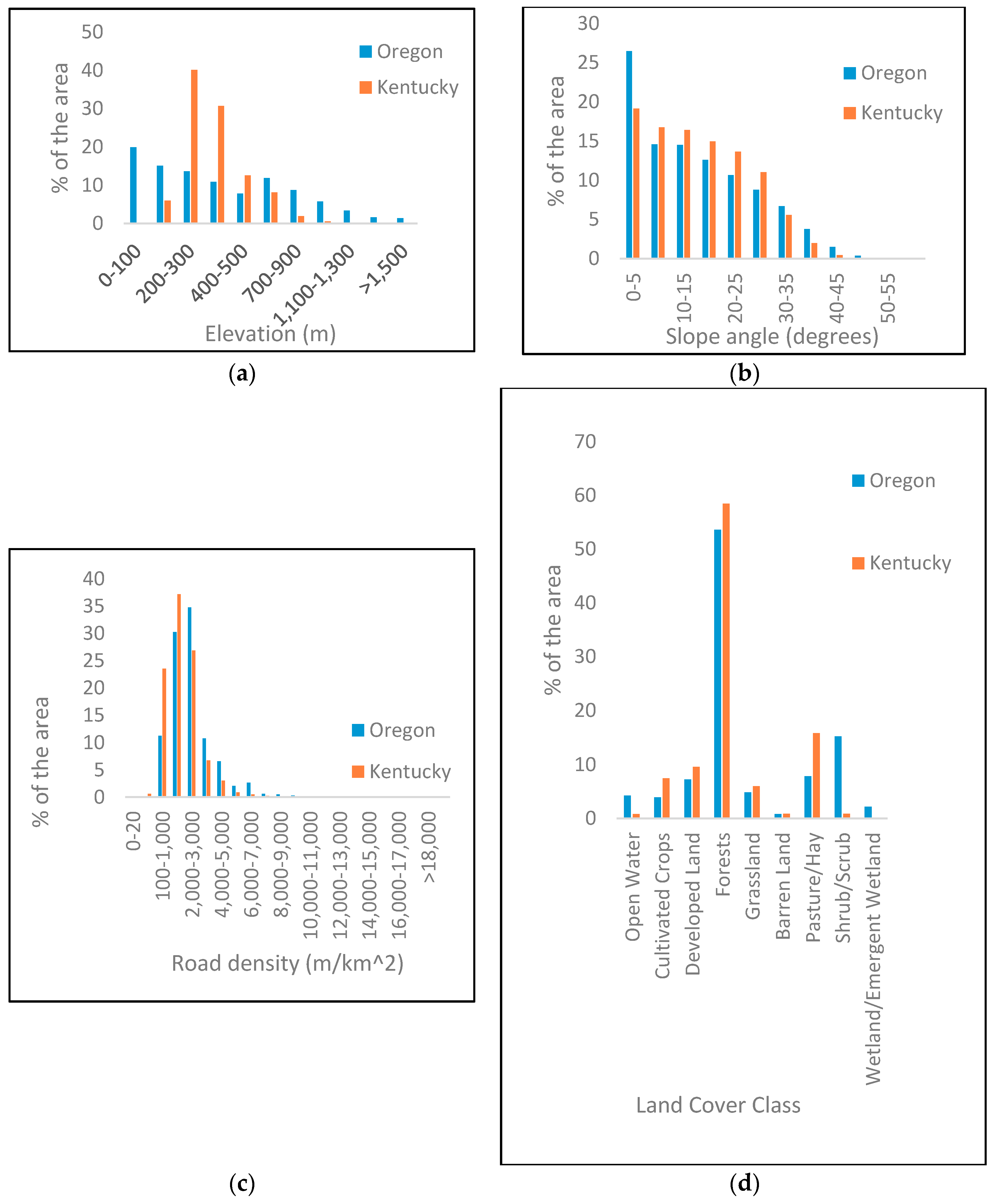
Geosciences 08 00326 g001
Figure 2. Frequency distributions of (a) elevation; (b) slope angle; (c) road density; and (d) land cover in the two study areas.
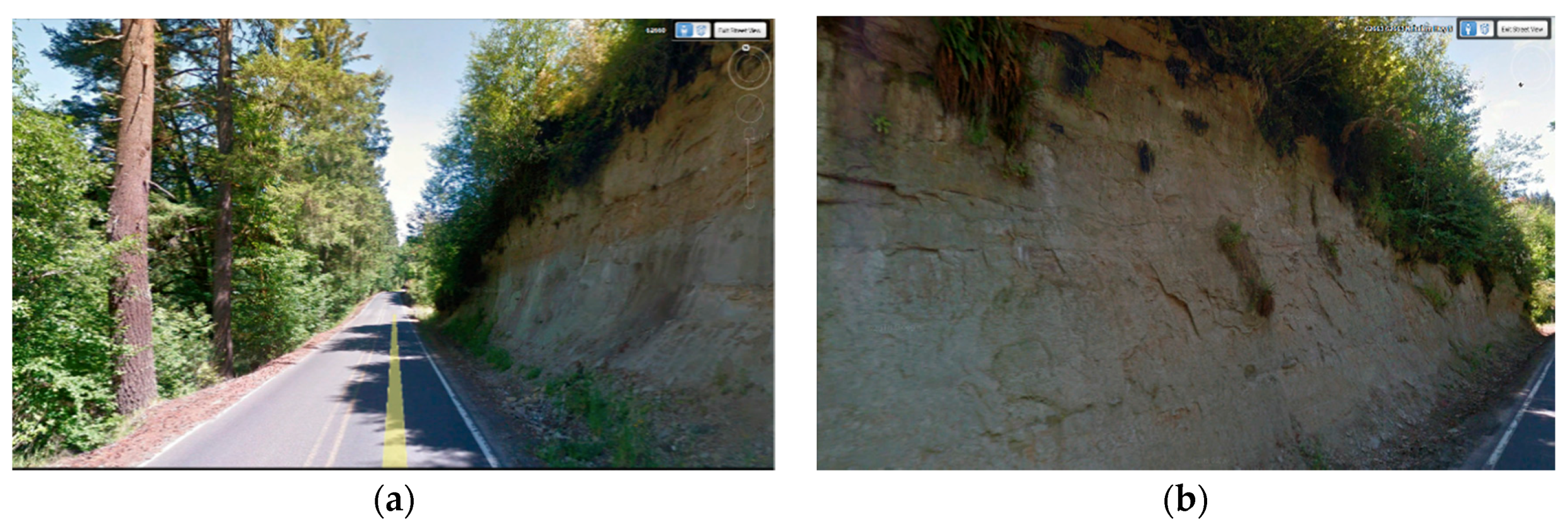
Geosciences 08 00326 g002
Figure 3. (a,b) Images of two sample locations that were excluded from the study due to the presence of exposed rock (Google Earth, 2018).
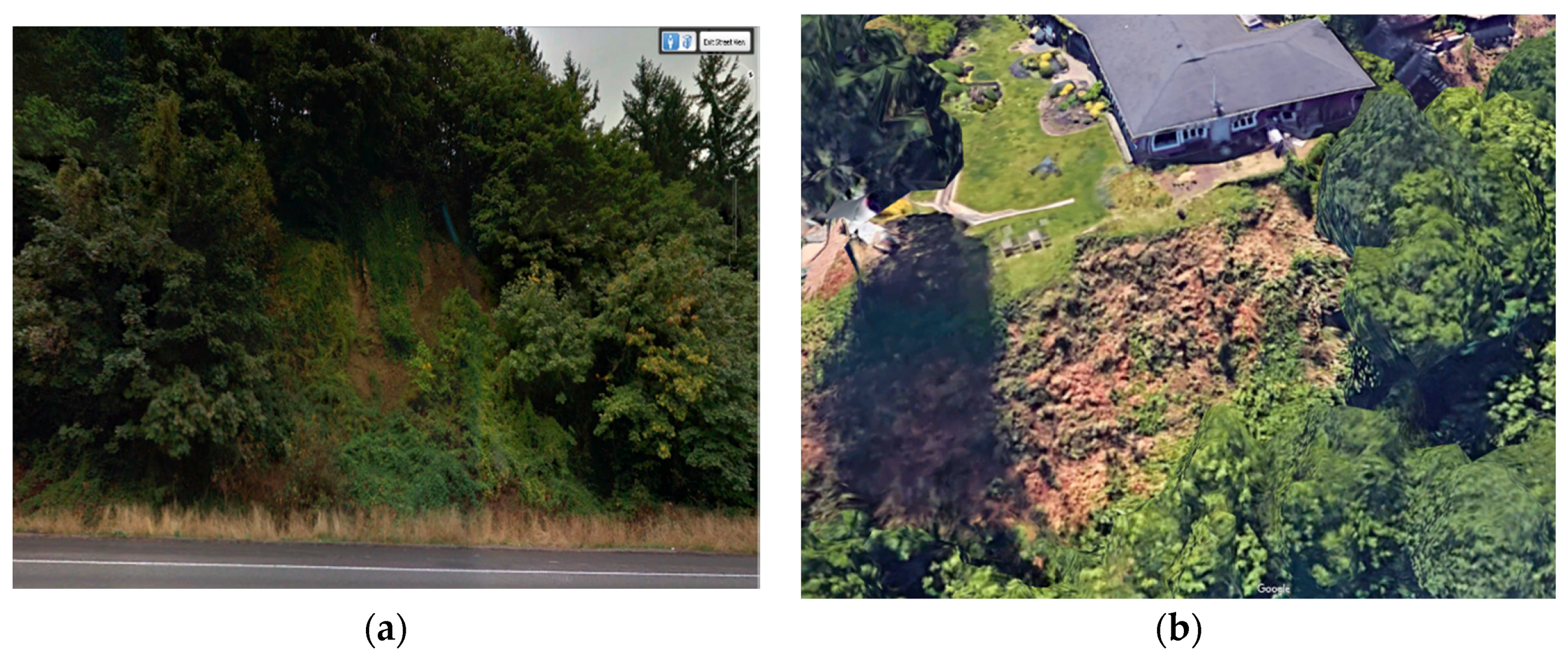
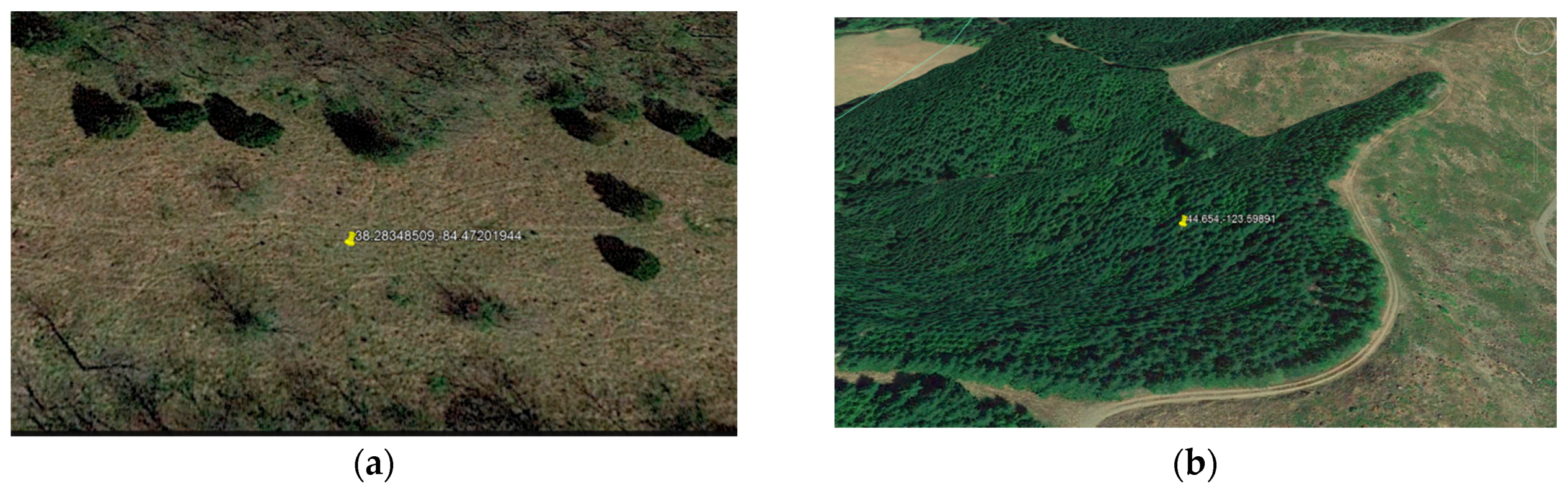
Geosciences 08 00326 g003
Figure 4. (a,b) May 2018 images of two selected soil slide sites (Google Earth, 2018).
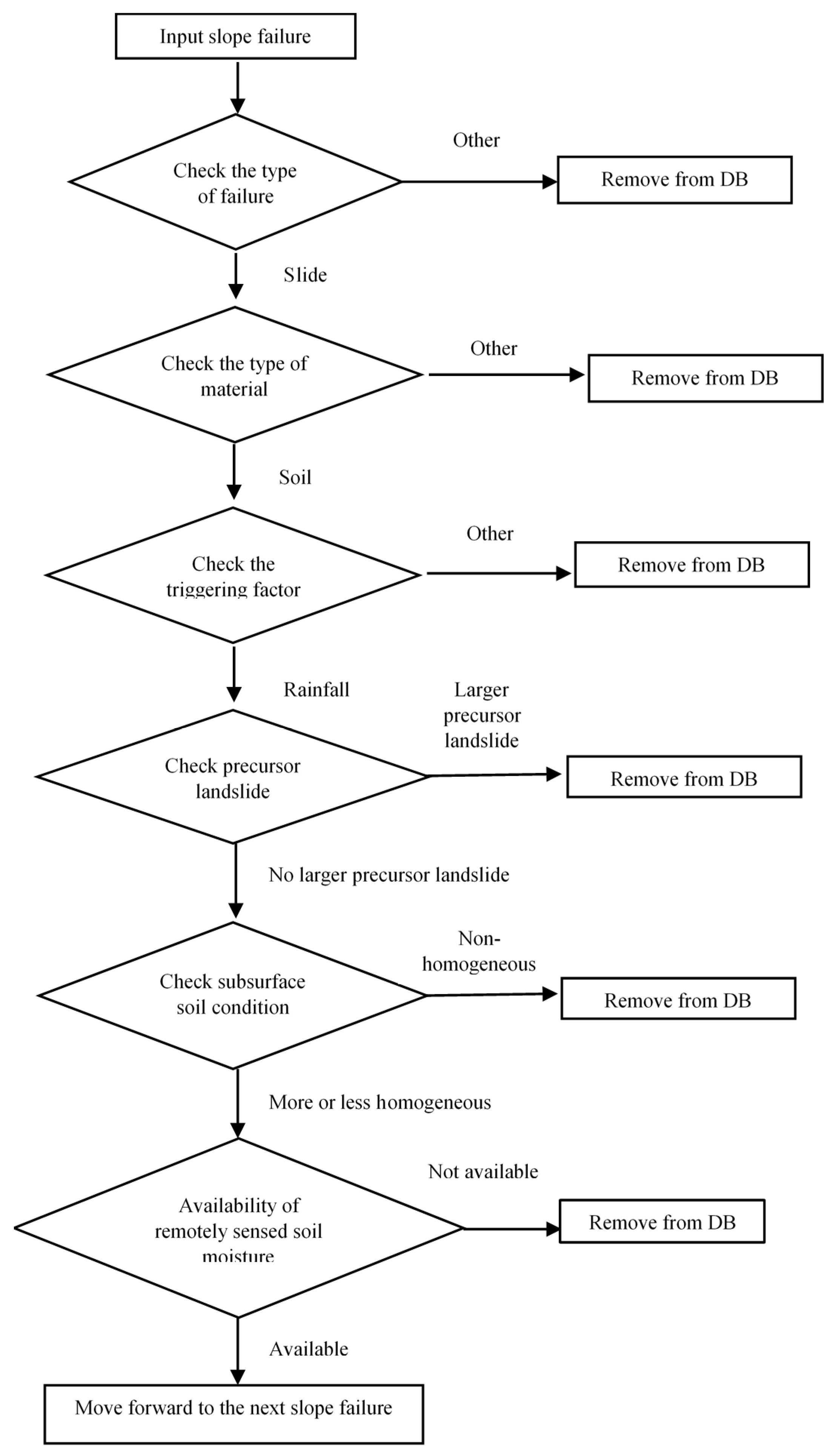
Geosciences 08 00326 g004
Figure 5. Procedure for selecting soil slide sites for this study.
Geosciences 08 00326 g005
Figure 6. (a,b) Two randomly selected non-soil slide locations used in the study (Google Earth, 2018).
Geosciences 08 00326 g006
Figure 7. Selected non-soil slides from (a) Oregon, USA, and (b) Kentucky, USA.
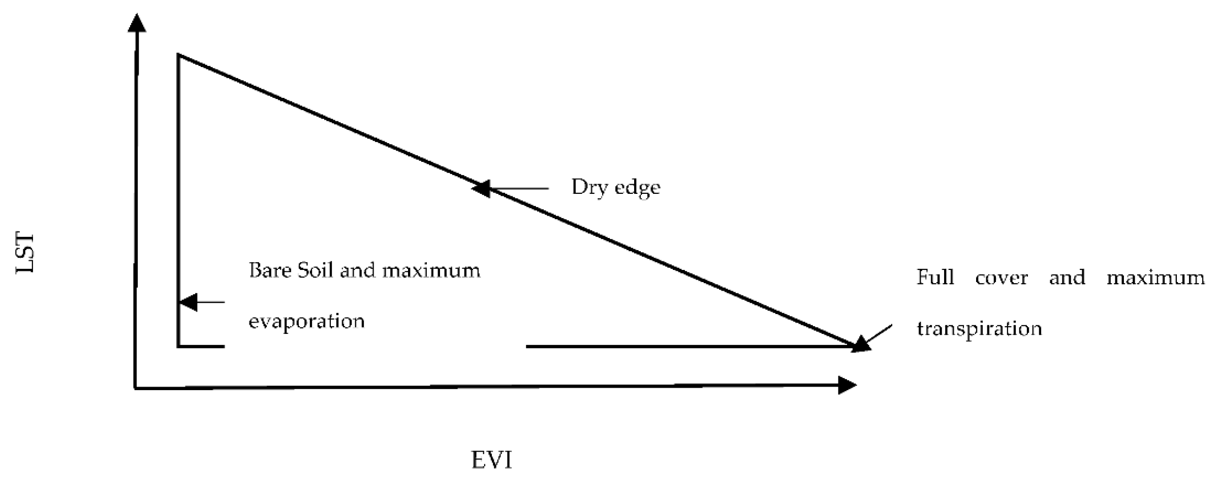
Geosciences 08 00326 g007
Figure 8. Triangular relationship between land surface temperature (LST) and the enhanced vegetation index (EVI).
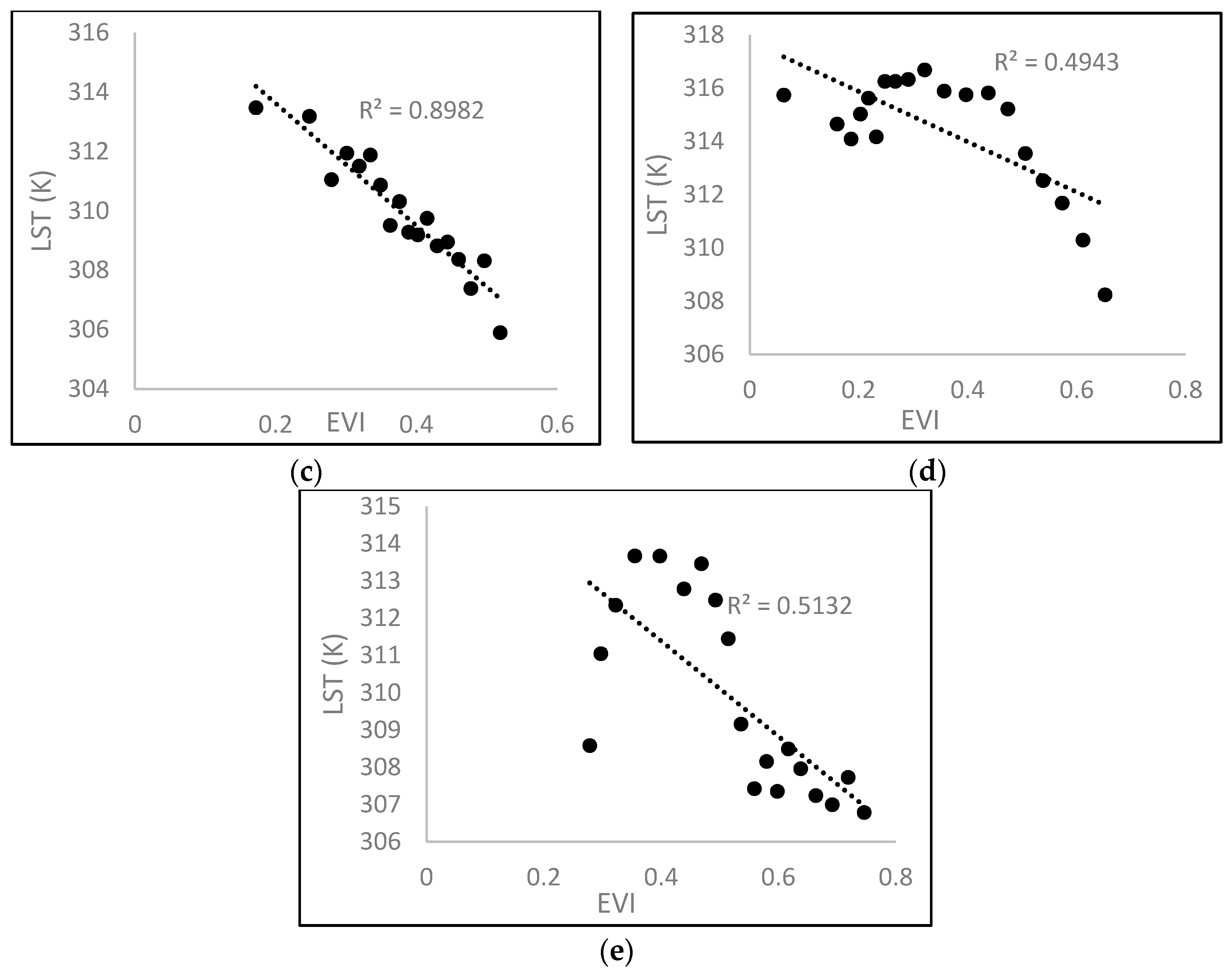
Geosciences 08 00326 g008
Figure 9. Dry edge parameters of (a) the top window of Oregon; (b) the middle window of Oregon; (c) the bottom window of Oregon; (d) the top window of Kentucky; and (e) the bottom window of Kentucky.
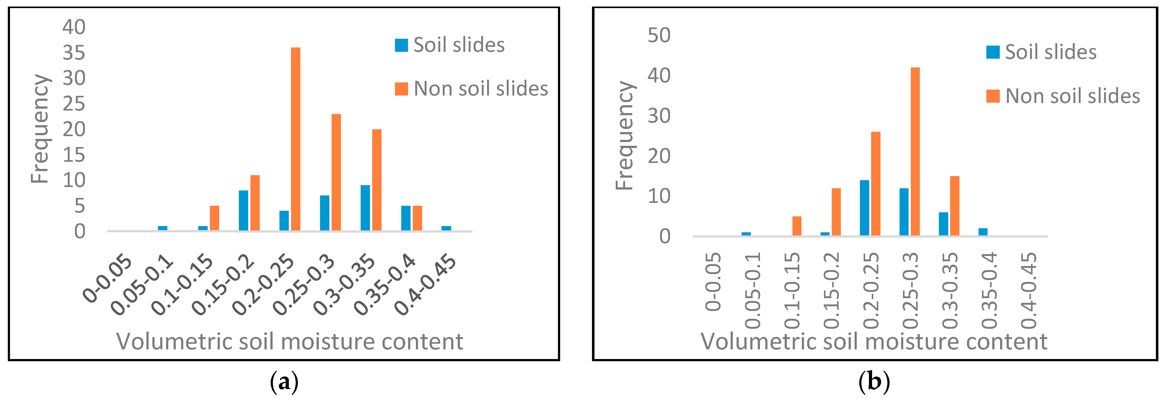
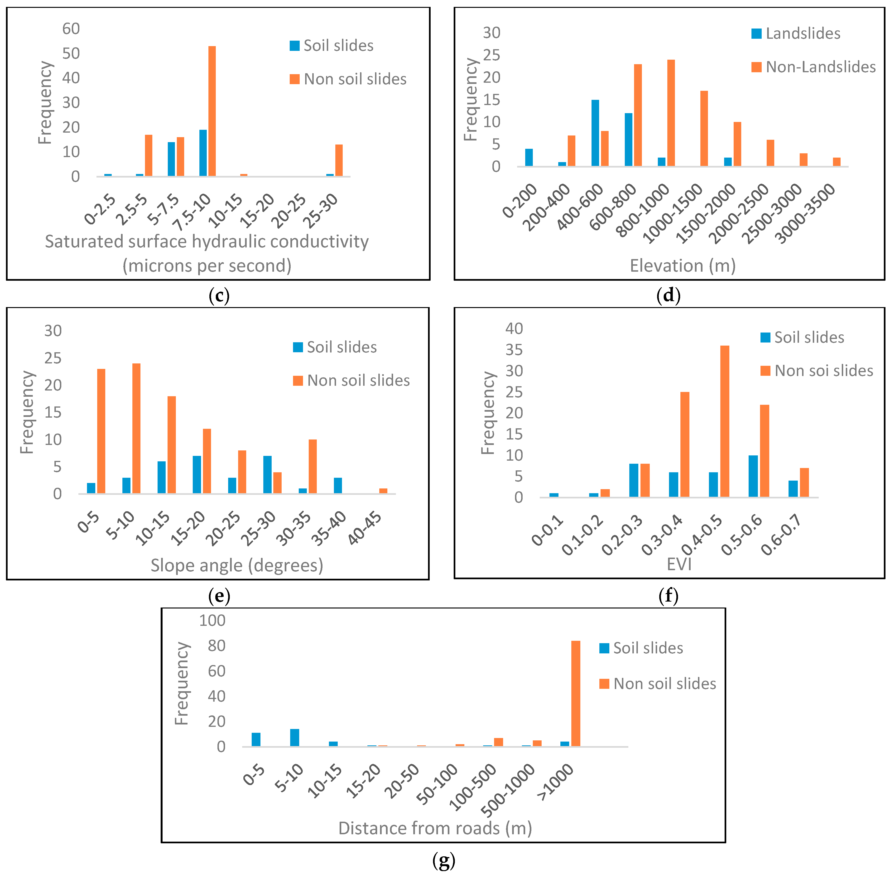
Geosciences 08 00326 g009aGeosciences 08 00326 g009b
Figure 10. Frequency distribution of (a) downscaled soil moisture; (b) undownscaled soil moisture; (c) saturated surface hydraulic conductivity; (d) elevation; (e) slope angle; (f) EVI; and (g) distance from roads.
Geosciences 08 00326 g010aGeosciences 08 00326 g010b
Figure 11. Variation of probability of failure with distance to roads (a) under low and high soil moisture contents; and (b) at low and high distances from roads.
Geosciences 08 00326 g011
Figure 12. Distribution of the predicted probability of failure at the soil slide and non-soil slide locations.
Geosciences 08 00326 g012
Figure 13. Selection of the failure probability threshold by maximizing the classification accuracy.
Geosciences 08 00326 g013
Figure 14. Classification of soil slides in (a) Oregon and (b) Kentucky.
Geosciences 08 00326 g014
Figure 15. (a) Frequency distribution of soil moisture at a 20-m distance from roads and (b) the variation of soil moisture thresholds for soil slide occurrence with distance from roads within a 20-m influence zone.
Geosciences 08 00326 g015
Table 1. Correlation matrix of the explanatory variables.
VariableElevation (m)SlopePresence of Clay Soil Type (Categorical Variable)Presence of Silt Soil Type (Categorical Variable)Presence of Gravel Soil Type (Categorical Variable)Enhanced Vegetation Index (EVI)Downscaled Soil Moisture
Elevation (m)-0.17−0370.030.46−0.002−0.03
Slope0.17-−0.28−0.030.41−0.040.07
Presence of clay soil type (categorical variable)−0.37−0.28-−0.70−0.500.030.05
Presence of silt soil type (categorical variable)0.03−0.03−0.70-−0.28−0.03−0.04
Presence of gravel soil type (categorical variable)0.460.41−0.50−0.28-0−0.02
EVI−0.002−0.040.03−0.030-−0.23
Downscaled soil moisture−0.030.070.05−0.04−0.02−0.23-
Undownscaled soil moisture−0.020.040.070−0.11−0.160.83
Saturated surface hydraulic conductivity (microns per second)0.420.42−0.44−0.150.770.02−0.09
Distance from roads (m)0.670.19−0.440.060.52−0.02−0.19
Proximity to drainage (m)−0.05−0.140.18−0.08−0.140.260.01
Drainage density (m−1)0.320.36−0.310.120.27−0.17−0.02
TWI−0.19−0.600.090.08−0.210.04−0.06
VariableUn-Downscaled Soil MoistureSaturated Surface Hydraulic ConductivityDistance from Roads (m)Distance to Drainage (m)Drainage Density (m−1)Topographic Wetness Index (TWI)
Elevation (m)−0.020.420.67−0.050.32−0.19
Slope0.040.420.19−0.140.36−0.60
Presence of clay soil type (categorical variable)0.07−0.44−0.440.18−0.310.09
Presence of silt soil type (categorical variable)0−0.150.06−0.080.120.08
Presence of gravel soil type (categorical variable)−0.110.770.52−0.140.27−0.21
EVI−0.160.02−0.020.26−0.170.04
Downscaled soil moisture0.83−0.09−0.190.01−0.02−0.06
Undownscaled soil moisture-−0.16−0.21−0.050−0.05
Saturated surface hydraulic conductivity (microns per second)−0.16-0.57−0.09−0.19−0.20
Distance from roads (m)−0.210.57-−0.18−0.16−0.10
Proximity to drainage (m)−0.05−0.09−0.18-−0.06−0.07
Drainage density (m−1)0−0.19−0.16−0.061−0.21
TWI−0.05−0.20−0.10−0.07−0.21-
Table 2. Statistics of the explanatory variables. EVI: Enhanced Vegetation Index.
VariableSoil Slide LocationsNon-Soil Slide Locations
MeanStandard DeviationMeanStandard Deviation
Downscaled soil moisture (m3/m3)0.27870.07500.25230.0585
Undownscaled soil moisture (m3/m3)0.26820.05190.25030.0478
Saturated surface hydraulic conductivity (microns per second)7.844.1510.047.39
Slope angle (degrees)20.9312.2913.349.68
Elevation (m)189100335200
EVI0.40200.15680.44030.1105
Distance from roads (m)25763766767511
Table 3. The distribution of soil types at soil slide and non-soil slide locations.
Soil Type% Soil Slide Locations% Non-Soil Slide Locations
GM (silty gravel)3.035
GC (clayey gravel)016
ML (low plasticity silt)27.2714
MH (high plasticity silt)014
CL (low plasticity clay)27.2729
CH (high plasticity clay)42.4222
Table 4. Parameter estimates, standardized parameter estimates, t-statistics, and p-values of the logistic regression model with all of the explanatory variables.
VariableParameter EstimateStandardized Parameter Estimatet-Statisticp-Value
Intercept−2.54−0.420.67
Downscaled soil moisture17.471.052.440.01
Elevation (m)−0.01−1.92−2.010.04
Slope angle (degrees)0.181.922.760.01
Distance from roads (m)−0.003−19.86−3.300.001
Saturated surface hydraulic conductivity (microns per second)−0.38−2.55−1.710.09
Presence of silt soil type (ML and MH)5.802.551.510.13
Presence of clay soil type (CL and CH)3.351.650.900.37
EVI−2.42−0.29−0.590.56
Table 5. Parameter estimates, standardized parameter estimates, t-statistics, and p-values of the best performing logistic regression model with downscaled soil moisture content.
VariableParameter EstimateStandardized Parameter Estimatet-Statisticp-Value
Intercept2.38-1.030.30
Downscaled soil moisture12.480.721.710.09
Elevation (m)−0.01−2.03−2.320.02
Slope angle (degrees)0.171.792.980.003
Distance from roads (m)−0.009−65.37−2.440.01
Saturated surface hydraulic conductivity (microns per second)−0.52−3.43−2.610.009
Presence of silt soil type (ML and MH)3.321.441.970.05
Downscaled soil moisture × Distance to roads0.0235.671.960.05
Table 6. Parameter estimates, standardized parameter estimates, t-statistics, and p-values of the best performing logistic regression model with undownscaled soil moisture content.
VariableParameter EstimateStandardized Parameter Estimatet-Statisticp-Value
Intercept0.54-0.200.84
Undownscaled soil moisture12.150.571.480.14
Elevation (m)−0.007−1.48−1.980.05
Slope angle (degrees)0.141.472.990.003
Distance from roads (m)−0.002−16.24−3.640.0003
Saturated surface hydraulic conductivity (microns per second)−0.36−2.46−2.350.02
Presence of silt soil type (ML and MH)2.120.941.770.08
Table 7. Parameter estimates, standardized parameter estimates, t-statistics, and p-values of the best performing logistic regression model with proximity to drainage accessories.
VariableParameter EstimateStandardized Parameter Estimatet-Statisticp-Value
Intercept6.85-2.270.02
Distance to drainage accessories (m)−0.009−1.52−1.390.16
Elevation (m)−0.026−5.21−2.620.01
Slope angle (degrees)0.161.693.060.002
Distance from roads (m)−0.002−13.41−3.490.0005
Saturated surface hydraulic conductivity (microns per second)−0.37−2.49−1.810.07
Distance to drainage × Elevation1.68 × 10−53.161.810.07
Table 8. Parameter estimates, standardized parameter estimates, t-statistics, and p-values of the best performing logistic regression model with drainage density.
VariableParameter EstimateStandardized Parameter Estimatet-Statisticp-Value
Intercept0.81-1.000.32
Drainage density (m−1)−0.48−0.60−1.900.06
Elevation (m)−0.013−2.46−3.860.0001
Slope angle (degrees)0.151.674.080
Table 9. Parameter estimates, standardized parameter estimates, t-statistics, and p-values of the best performing logistic regression model with Topographic Wetness Index (TWI).
VariableParameter EstimateStandardized Parameter Estimatet-Statisticp-Value
Intercept−0.75-−0.240.81
Topographic Wetness Index0.440.811.640.1
Elevation (m)−0.007−1.35−1.850.06
Slope angle (degrees)0.182.012.990.003
Distance to roads (m)−0.002−15.62−3.770.0002
Saturated surface hydraulic conductivity (microns per second)−0.39−2.63−2.600.01
Presence of silt soil type (ML and MH)1.700.761.481.40
Table 10. Comparison of the performance of logistic regression models. AIC: Akaike information criterion; BIC: Bayesian information criterion.
Hydrological Variable in the ModelLog LikelihoodAICBIC
Downscaled soil moisture content−17.9051.874.92
Undownscaled soil moisture content−23.3360.680.89
Distance to drainage accessories (m)−22.3058.678.89
Drainage density (m−1)−49.71107.4118.98
Topographic Wetness Index−23.2860.680.79
Table 11. Classification accuracies of soil slide and non-soil slides for Oregon and Kentucky.
DatasetClassification Accuracy %
All data93.2
Oregon data95.7
Kentucky data80.5
Table 12. Classification accuracies of soil slide and non-soil slides for Oregon and Kentucky.
Oregon %Kentucky %
Soil slides81.895.5
Non-soil slides9095.7
Table 13. Confusion matrix for the results obtained with the soil slide classification model.
Predicted Class
True class Soil SlidesNon-Soil Slides
Soil slides303
Non-soil slides694

