1. Introduction
In recent decades, the airborne gravimetry technique has become more and more important for the acquisition of local gravity field data [
1,
2]. This is due to the fact that it permits investigating large areas, of about 100 km × 100 km, by a few days survey and at a relatively low cost, if compared to other techniques, such as ground point-wise measurements, which can be quite time consuming and expensive. Another advantage of using this technique is linked to the possibility of performing measuring campaigns in almost every kind of challenging environments, e.g., mountains, rain forests, polar areas [
3,
4].
Airborne gravimetry did not become fully operational until the advent of the Global Positioning System (GPS) at the end of the 1980s. This technology, in fact, permitted solving the major problem of precise estimation of the aircraft position and led to the improvement of the existing measurement systems and consecutively to the spread of the airborne gravimetry for both the geophysical exploration and geodetic applications. The new accuracy after the advent of GPS were of few mGal (1 mGal =
ms
2) at a spatial resolution of 5–6 km [
1]. Thanks to this technological advancement, apart from the classical stabilized platform system, various measuring systems started to be deployed like the Strapdown Inertial Navigation System, which is based on a set of three orthogonal accelerometers and three gyroscopes or the system based on a combination of GPS and Inertial Measurement Units, used to determine all the components of the gravity vector [
5,
6,
7,
8]. Nowadays, even if different research groups were able to show that strapdown systems can basically produce the same gravity quality of the stabilized platform one [
1,
9,
10] (also for production-oriented campaigns under challenging conditions), the latter is still considered as the standard technique, especially for geophysical applications.
As stated before, airborne gravimetry is, at present, widely adopted for multiple applications in both geodesy and geophysics. Among the different geodetic applications, one of the most important is the local geoid determination [
11] in which airborne gravimetry observations are generally combined with satellite gravimetry data, the latter being more reliable to provide information about the low frequency of the gravitational field signal. Another important application of airborne gravimetry is the so called polar gaps filling. The gravity field of the polar regions is in fact of primary importance for Earth’s Global Gravity field Models (GGMs), but also for providing information on the geology of those regions and for navigation and orbit determination, since the recent satellite gravity field missions such as CHAMP (Challenging Minisatellite Payload), GRACE (Gravity Recovery And Climate Experimen) and GOCE (Gravity field and steady-state Ocean Circulation Explorer) are all strongly affected by the gravity field of polar regions, as they had non-polar orbits that consequently led to polar gaps in their data coverage [
12]. The recent European Space Agency PolarGAP [
13] project, for example, was carried out in the period 2015–2016 with the principal aim to adopt airborne gravity surveys over the southern polar region to cover the polar gap of GOCE in this area (south of
S).
On the other hand, in regards to the geophysical applications, airborne gravimetry is mainly used for regional geological studies and for resources exploration. For the latter application, frontier regions or near shore regions are in fact more and more frequently investigated requiring the adoption of airborne gravimetry, which results in the most suitable gravity measuring technique.
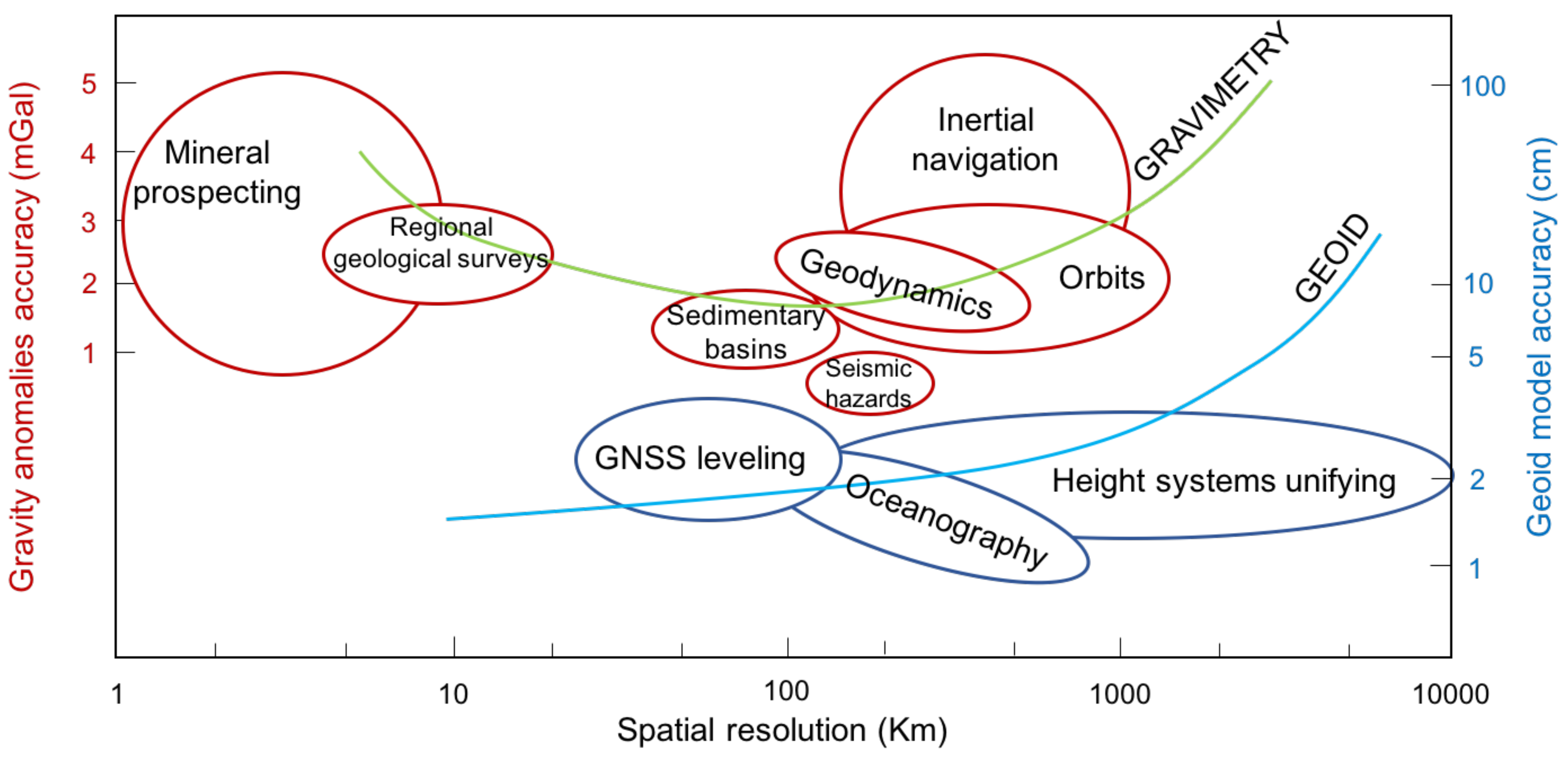
Figure 1 reports a schematic representation of the required accuracies and resolutions for different airborne gravimetry applications. It can be noticed how these two variables can range in a quite large set of possible values, depending on the purpose of the data acquisition: for example, mineral prospecting requires accuracies of few mGal at a spatial resolution of 1–5 km, similarly to regional geological surveys, while geodetic applications related to geoid modeling for various scopes require much lower spatial resolutions (hundreds of km) and an accuracy in terms of geoid of a few centimeters.
Due to these differences, it has to be underlined that the kind of application is of paramount importance since it directly influences the survey design and planning. The type of observation, the required accuracy, the area coverage, the resolution and the flight path as well as the definition of the instrumentation to be used are all part of the survey design and are strictly dependent on the scope of the acquisition. As it is obvious, for highly-accurate high-resolution results, the airborne acquisition should be performed as slow as possible and with a very dense acquisition path, thus increasing the survey cost. For this reason, in the present work, we develop an airborne survey simulator [
14] that, starting from a simulated airborne gravimetric signal, permits evaluating the accuracy of the acquired gravitational field. In more detail, in the following
Section 2, all the aspects related to the simulation of airborne gravity observations as well as those related to the processing procedure are briefly described. Then,
Section 3 is dedicated to the presentation of the numerical tests performed along with some considerations on the obtained results. In the end, some relevant conclusions and essential remarks are drawn in
Section 4.
2. Methodology
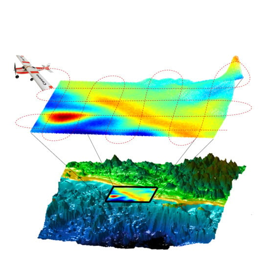
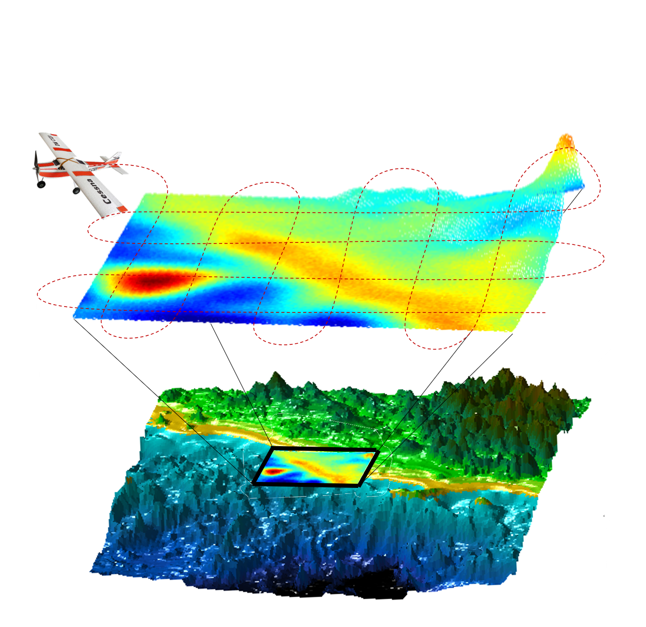
The airborne gravimetric survey simulator developed within this work and presented in this section is a software package thought of as a useful tool to easily simulate a gravimetric signal, i.e., a set of gravity disturbances, on points over a certain flight track. The final objective of this project is the definition of a procedure to optimally plan the airborne survey, according to the required final accuracy and spatial resolution. Thus, once the signal had been simulated, the processing technique described in [
15] is applied, thus recovering the expected filtered gravitational field, together with its predicted accuracy. The whole methodology used to process the simulated signal is summarized here for the sake of completeness; however, the interested reader can refer to the already cited [
15].
The simulator is based on the concept that, once provided, the essential parameters such as the coordinates of the investigated area, the flight starting point, the aircraft velocity, sampling rate, tracks inter-spacing and trajectory planimetric inclination angle, it is possible to reconstruct the aircraft path and the observation points within the interested area. Moreover, considering that standard airborne survey for geophysical applications are constituted by tracks oriented along two perpendicular directions (namely traverse lines and control lines), the simulator allows the user also to add these crossing lines, setting their desired inter-spacing. A note has to be taken on the fact that curves between two consecutive tracks have not been considered here because real airborne gravimetric observations taken along curved paths are never included in the processing phase due to the extremely dynamic environment in which they are acquired that degrades the quality of the measurements. It should be also observed that the simulator will predict the final accuracy along the aircraft trajectory; for this reason, at least in the current work, the effect of the flight altitude is not investigated.
Once the coordinates of the observation points are generated, the simulator creates the observed signal of gravity disturbances
, along the aircraft trajectory, by performing a spherical harmonic synthesis,
, of a Global Gravity field Model (GGM) up to its maximum degree/order
and adding to it a residual terrain correction,
, and a colored noise
:
In more detail, the global model term, namely
, is computed from the coefficients
and
given by the GGM by means of the following well-known [
16] expression:
where
G is the universal gravitational constant, equal to
m
3kg
−1s
−2, M is the Earth mass (
kg),
a is the Earth semi-major axis (taken here equal to 6,378,137 m),
is the fully normalized associate Legendre function of degree
m and order
ℓ, and
are the geocentric coordinates of the point in which
should be computed.
The second term of Equation (
1), i.e., the residual terrain correction [
17]
, is evaluated as the difference between two terrain corrections: the first one computed from a high resolution Digital Terrain Model (DTM) and the second one computed from a smoothed DTM obtained by applying a moving average window to the high resolution DTM. As reported in [
18], the window size
K is related to
by the following relation:
Both the terrain corrections within this work have been computed using a hybrid algorithm that exploits a combined Fast Fourier Transform–prisms approach, working in spherical approximation [
19].
As for the colored noise , it is generated by considering the following hypothesis:
observation along the same flight line are correlated, while observations of different flight lines are supposed to be independent;
the observation noise is zero mean and stationary, namely and , where d is the distance between two points on the same flight line.
Basically, a theoretical noise covariance function
is set by the user, and, for each flight line, an along track error sample is generated as:
where
is a matrix such that
, here obtained by means of Cholensky decomposition,
is the covariance matrix between points
, and
is a vector containing uncorrelated samples from a normal distribution. A comment is required at this point, in fact while the first hypothesis is surely well verified when dealing with real acquisitions, the second one, namely the hypothesis to have
, can be considered questionable. It is in fact well known that the gravimeter observations are affected from biases and trends. However, we will suppose in the current work that the observations, biases, and trends (for sufficiently long paths, i.e., more than 80 km) can be proficiently repaired by exploiting information coming from satellite observations as shown in [
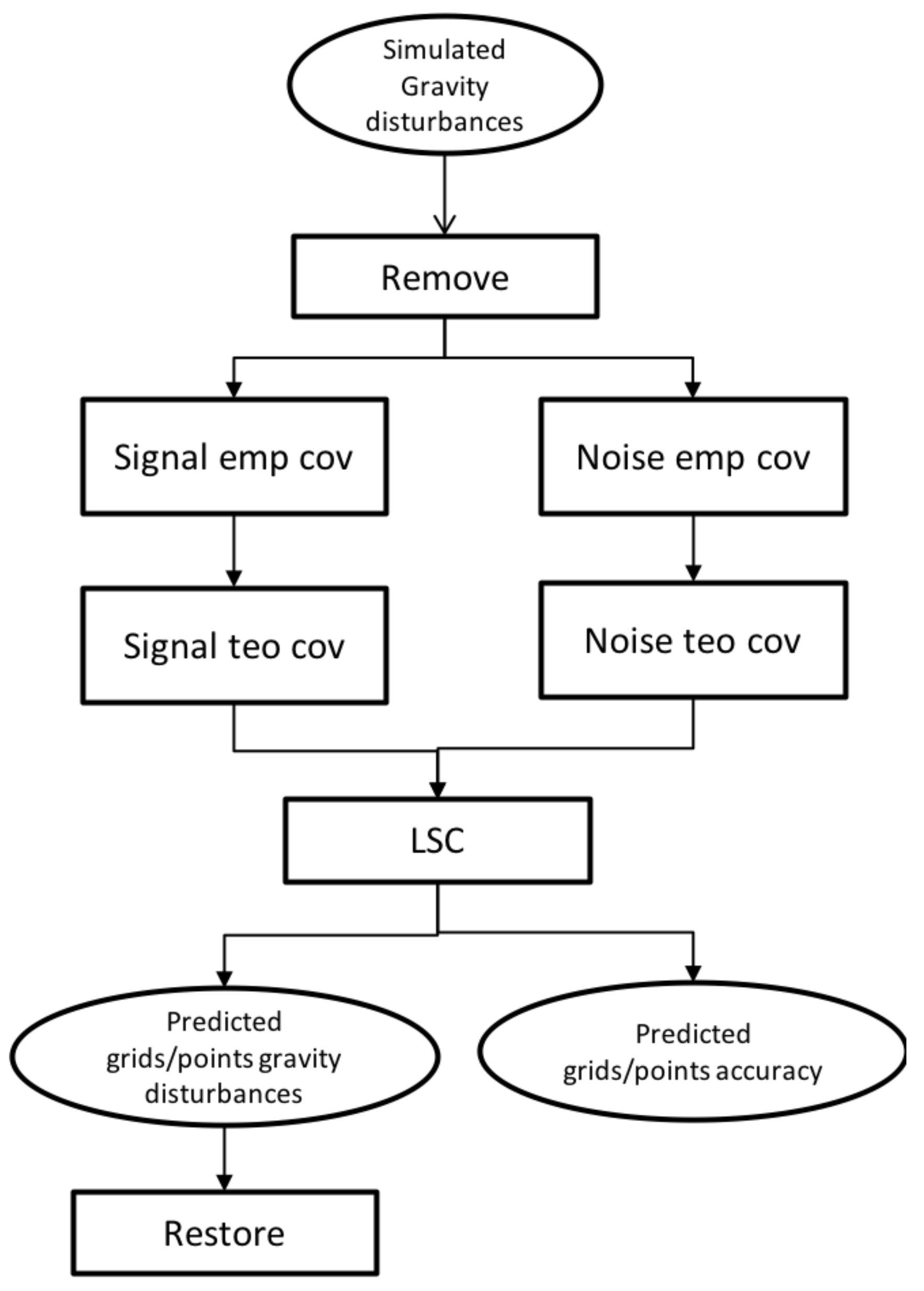
15]. As a consequence, we are entitled to apply also this second approximation in the following. In this way, the simulated gravity disturbances are equivalent to an hypothetical filtered aerogravimetric signal that can be processed with a remove–compute–restore like procedure. The proposed processing scheme is shown in
Figure 2 and outlined in the following paragraph.
Starting from our simulated filtered gravity disturbances along the aircraft trajectory, the first step to be performed is the so called remove. It consists of subtracting from the simulated signal the contribution of a global gravity model for the low frequencies and of a global model of the gravitational effect of the topography for the medium-high frequencies . The former, i.e., , is obtained from a chosen GGM with a spherical harmonic synthesis up to a certain intermediate degree (e.g., here set to 360). The latter, namely , instead is derived from a spherical harmonic synthesis of a global model of terrain effect from to the maximum degree of the model . After this phase, the reduced observations, which are basically , are characterized by a zero mean, a smaller amplitude and short spatial correlation with respect to the original signal.
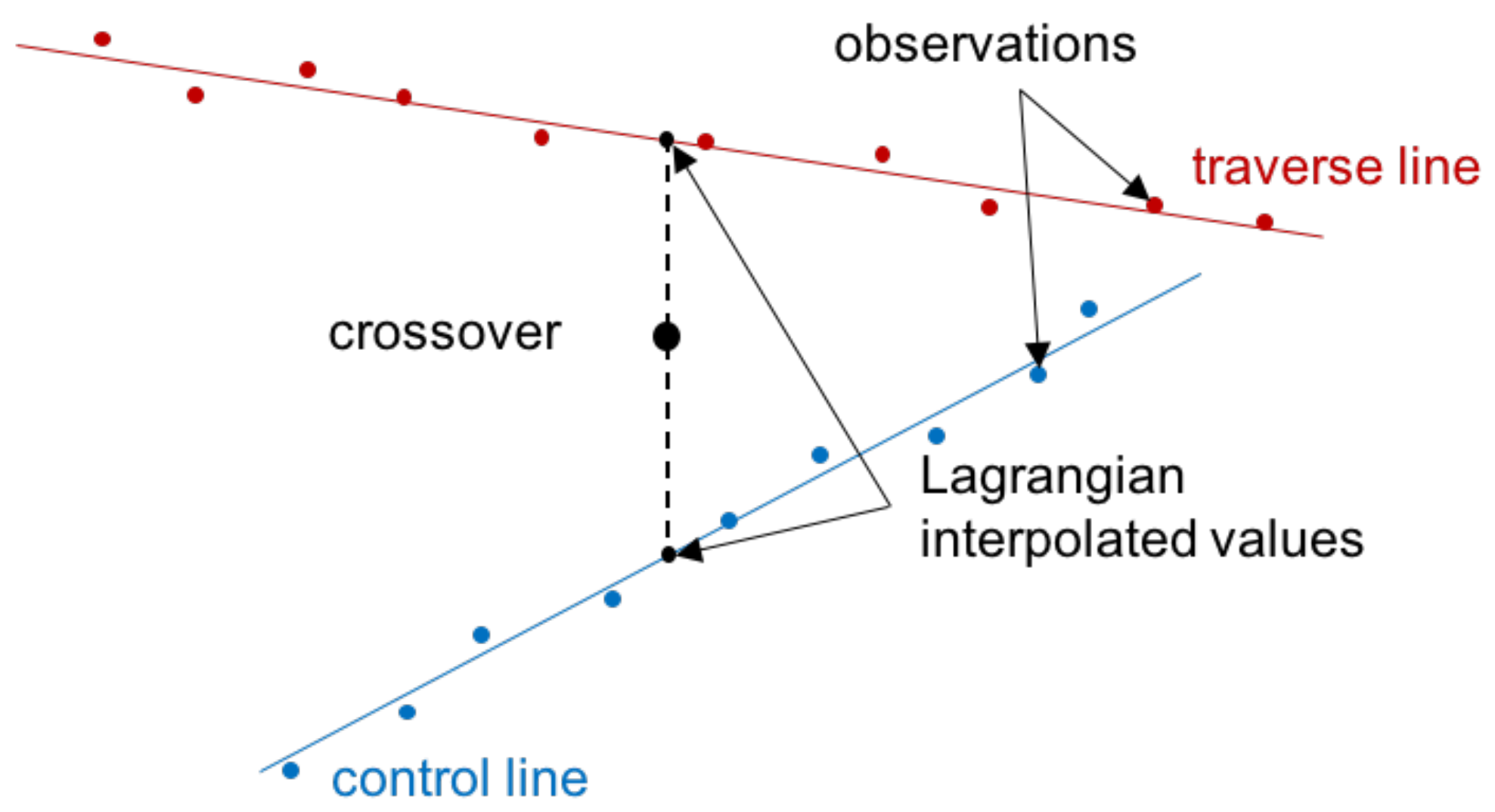
The subsequent compute step consists of the Least Squares Collocation prediction of the filtered residual field, which is used to predict the signal on the same or others’ chosen points (e.g., a grid). In order to perform this step, both the signal and the noise covariance functions should be properly modeled. Within the proposed procedure, the former, i.e., the signal covariance, is empirically obtained directly from the observations while the latter, namely the noise one, is estimated from the crossover analysis, i.e., from the signal difference at intersections between two perpendicular flight tracks. Of course, the quality of this error covariance increases with the number of available crossovers, in geophysical application surveys, up to a few thousand crossovers can be available, thus allowing for a quite realistic error estimate.
In order to model the noise covariance by means of this crossover analysis procedure, each aircraft track is modeled as a straight line, estimating the parameters with a Least Squares adjustment. This modeling is necessary to identify the intersection points between the tracks. Then, for each crossover point, the gravity signal in correspondence of the intersection is evaluated (separately for the two considered lines) by means of a Lagrangian interpolation. Finally, the residual is derived as the difference between the two obtained values of the signal (see
Figure 3).
Once all the residuals at the crossovers have been evaluated, they can be associated with the error of the filtered gravity disturbances, which can be used to compute the empirical along-track error covariances. Now, under the hypothesis that the stochastic properties of the along track error are stationary, it is possible to apply an average on the covariances of all the lines to obtain the final estimate of the empirical along-track error covariance function. This operation guarantees the estimate of a robust error covariance, a property that can not be valid for a single flight line, due to the general limited number of error samples retrievable.
Note that, in order to apply this methodology, and therefore to properly estimate the error covariance function, the airborne survey should contain perpendicular lines. This is quite typical for an airborne gravity survey, since up to now the crossovers have been in general required to remove from the observed field the well known biases and trends. However, it should be observed here that, for the proposed procedure, this acquisition scheme is not strictly required anymore, since both the biases and the long wavelength trends, if the survey is sufficiently large (i.e., of the order of 80 km), can be properly adjusted from satellite derived information coming from the CHAMP, GRACE and GOCE missions.
Both the signal and noise covariance functions are then modeled by means of a linear combination of Bessel function of first order since these functions can properly describes the typical oscillations that characterize the empirical gravity field covariance and can assure the harmonicity of the out-coming field.
Finally, the full gravitational signal is obtained by restoring back the signal removed in the initial remove step.
3. Numerical Tests
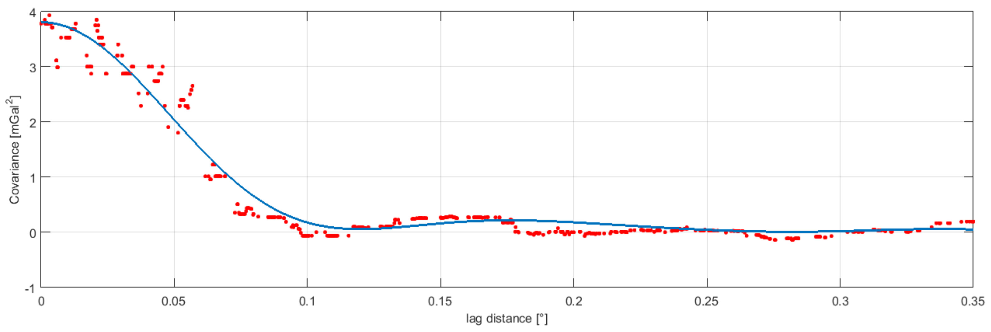
In order to start the airborne simulation, and analyze different scenarios, the fundamental operation is to properly set the initial noise error covariance function. Here, it has been obtained by directly analyzing, with the proposed crossover procedure, the raw observations of a real airborne survey performed within the framework of the CarbonNet project [
20]. In
Figure 4, the empirical and the theoretical covariance functions obtained and used in the sequel to simulate the observation errors are displayed.
It can be seen from the reported covariance function that the observation error has a variance of mGal2 and a correlation length of about corresponding to km.
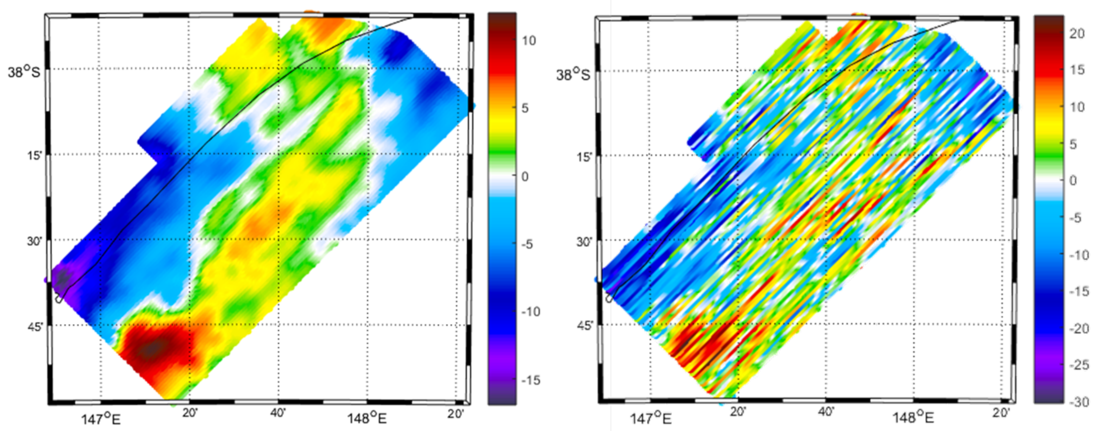
Before starting our analysis, we should also define the survey area, the distances between consecutive traverse and control lines, and the aircraft velocity. Within the first simulation, we considered the same area of the real CarbonNet acquisition. As for the other parameters, we will start by supposing a survey scheme again similar to the one used in the real airborne acquisition, i.e., with distances between traverse lines of 1 km and distances between two consecutive control lines of 10 km. The aircraft velocity is taken equal to 50 m/s. The simulated signal, once the remove step has been applied, with and without the noise realization, is shown in
Figure 5.
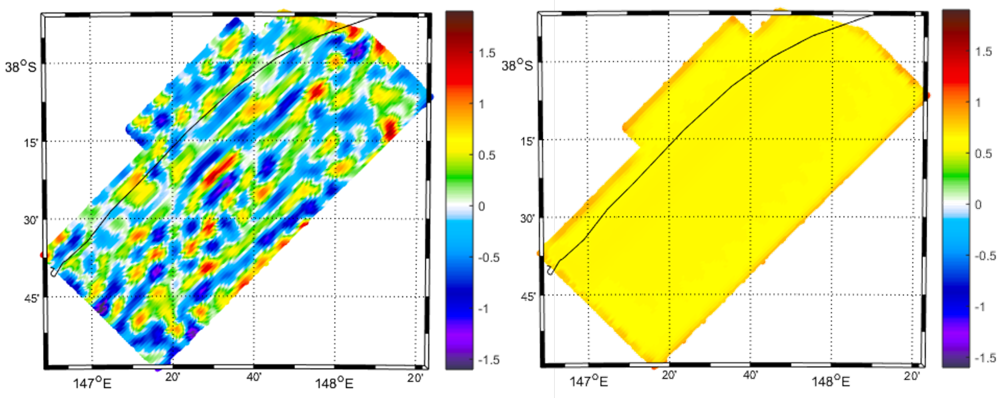
After carrying out the whole filtering procedure, we obtained a predicted accuracy of about
mGal (see
Figure 6), which is quite consistent with the actual difference between the reference and the predicted signal (the latter showing a standard deviation of
mGal). This first test has been performed just to prove, by means of real data, the reliability of the developed gravity survey simulator.
A first problem that we can analyze using the proposed simulation tool is the importance of having both the traverse and control lines within the survey. Basically, the control lines in our processing scheme have a dual impact on the final estimate: on the one hand, they allow for a correct error covariance modeling; on the other hand, they add useful independent observations to the set of input data. The former effect is evaluated here by considering within the Least Squares Collocation adjustment a simple white noise model (with a standard deviation of 1 mGal) instead of the correct noise covariance model, while the latter, namely the effect of the number of independent observations, is evaluated just by removing from the initial dataset the control lines’ observations. For both of these scenarios, the Least Squares Collocation adjustment is applied, and the obtained results are compared with the reference gravity signal. The results of these two tests show that ignoring the proper error covariance function in the Least Squares Collocation prediction, and considering instead a simple white noise model, has a small negative impact on the final estimate, degrading the final accuracy from mGal to mGal (standard deviation of the difference between retrieved field and reference one). As for the second scenario, i.e., modeling the error covariance as white noise and removing also the observations coming from the control lines, a more significant reduction in the final accuracy is obtained, from mGal to mGal (standard deviation of the difference between retrieved field and reference one).
We move now to a second simulation scenario: we considered in this case an area in Central Italy that extends between 11.95–12.65° East and 41.15–41.85° North, and we tried to retrieve the survey parameters minimizing the flight time (and therefore minimizing the flight cost), but always assuring an accuracy better than 1 mGal, i.e., simulating a possible scenario for the design of an airborne survey for exploration activities or regional geological investigations. For this purpose, a different combination of distances between traverse lines and control lines, and different velocities have been simulated and processed. Results are reported in the following
Table 1.
As expected, the worsening of the final predicted accuracy can be clearly seen due to the increasing of the space between two consecutive traverse lines (test ID from from 6 to 9). A slightly minor effect is the one due to the change in the aircraft velocity, where doubling the aircraft speed will decrease the expected accuracy from
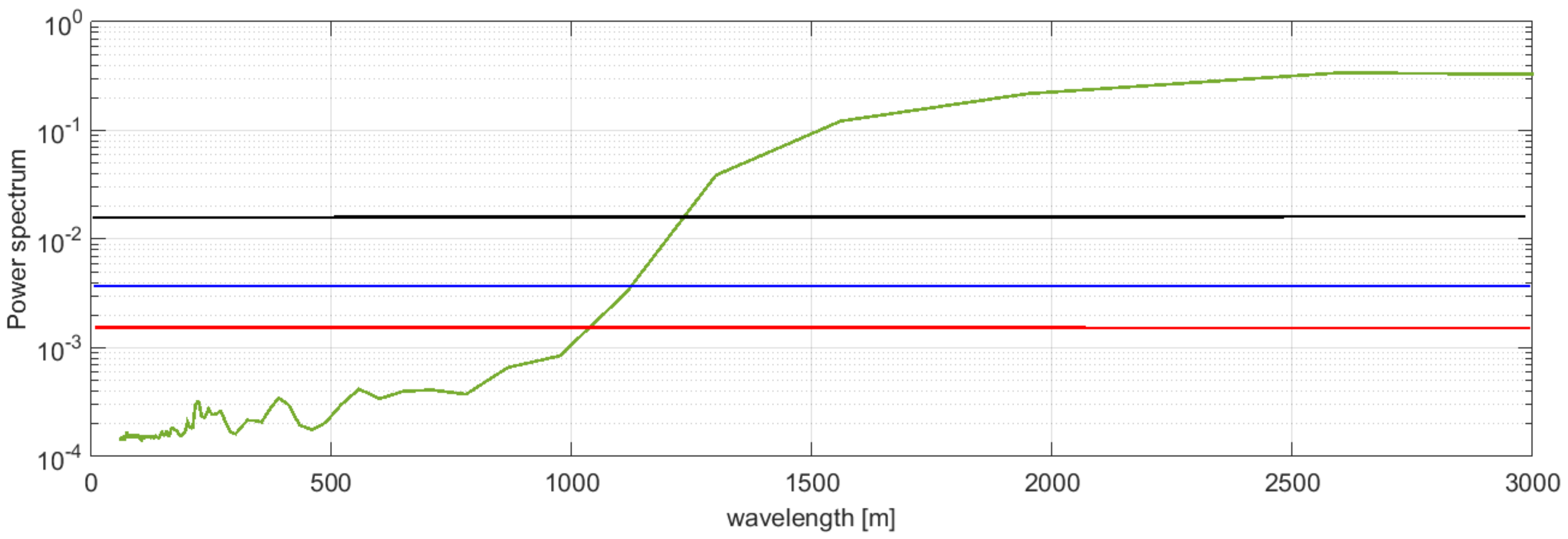
mGal to about 1 mGal. This is quite predictable since adding traverse lines would add a set of independent observations, while decreasing the speed will basically have the effect of increasing the number of correlated observations. In order to evaluate the achievable spatial resolution, we computed the signal power spectrum (supposing an isotropic behavior) and compared it with the power spectrum of a white noise with different variances (
Figure 7).
It can be seen that the mGal noise (red line) would allow in principle to recover wavelengths of the gravity field larger than about 1 km, which increase to for the 1 mGal noise (blue line) and to for the mGal (black line). It should be observed that of course this resolution is referred to the along track retrievable wavelengths. In fact, considering, for instance, test 9, where a traverse line spacing of 10 km has been used, the minimum retrievable spatial resolution will increase.
Summarizing the results obtained for this scenario, aiming for a final accuracy of 1 mGal (typical for surveys related to exploration activities or regional geological studies), we can say that the safer situation is of course a slow flight speed (50 m/s), with 1 km spacing between traverse lines and 10 km spacing between control lines. However, the predicted accuracies obtained show that the aircraft flight speed could probably be increased up to 75 m/s, thus reducing the flight time (and therefore the survey cost). Of course, the obtained results strictly depend on the area considered, in fact the estimate obtained from the Least Square Collocation Adjustment, is based on both the noise and the signal covariance, the latter being retrieved from the reduced signal itself.


