Article

Improved Interpretation of Marine Sedimentary Environments Using Multi-Frequency Multibeam Backscatter Data

by
Peter Feldens
1,*,
Inken Schulze
1,
Svenja Papenmeier
2,
Mischa Schönke
1 and
Jens Schneider von Deimling
3
1
Marine Geology, Leibniz Institute for Baltic Sea Research Warnemünde, 18119 Rostock, Germany
2
Alfred Wegener Institute, Helmholtz Centre for Polar and Marine Research, Wadden Sea Research Station, 25992 List/Sylt, Germany
3
Institute of Geosciences, Christian-Albrechts-Universität zu Kiel, 24118 Kiel, Germany
*
Author to whom correspondence should be addressed.
Geosciences 2018, 8(6), 214; https://doi.org/10.3390/geosciences8060214
Submission received: 8 May 2018 / Revised: 8 June 2018 / Accepted: 9 June 2018 / Published: 12 June 2018
(This article belongs to the Special Issue Geological Seafloor Mapping)

Abstract

:
Backscatter mosaics based on a multi-frequency multibeam echosounder survey in the continental shelf setting of the North Sea were compared. The uncalibrated backscatter data were recorded with frequencies of 200, 400 and 600 kHz. The results showed that the seafloor appears mostly featureless in acoustic backscatter mosaics derived from 600 kHz data. The same area surveyed with 200 kHz reveals numerous backscatter anomalies with diameters of 10–70 m deviating between −2 dB and +4 dB from the background sediment. Backscatter anomalies were further subdivided based on their frequency-specific texture and were attributed to bioturbation within the sediment and the presence of polychaetes on the seafloor. While low frequencies show the highest overall contrast between different seafloor types, a consideration of all frequencies permits an improved interpretation of subtle seafloor features.

1. Introduction

A reliable, repeatable and objective classification of seabeds, ultimately comprising both geological and biological habitats, continues to be an important issue for marine spatial planning and management as well as for research. Acoustic remote sensing by side scan sonar and multibeam echosounder obtains information on seafloor habitats based on measuring the intensity of acoustic signals backscattered from the seafloor [1,2]. The intensity of a backscattered signal depends on a number of geo-acoustic properties of the sediment surface and shallow subsurface, the water column, geometrical and technical parameters, and has been described by a number of physical and heuristic models [3,4,5]. The bulk backscattering level measured by the sonar comprises specular reflection, seafloor scatter and volume scatter and depends on the incidence angle and frequency of the acoustic wave. The angular dependence of backscatter levels has been used to characterize different seabeds [6,7]. A disadvantage of angular response curve (ARC)-based seafloor classification is their inherent half-swath width resolution (except for survey geometries with strongly overlapping survey lines) [8]. Therefore, ARCs are less sensitive to small-scale variations in seafloor composition and a strong synergy with backscatter mosaics corrected for the angular dependence exists, albeit this is rarely utilized [7]. A standard geological application utilizing backscatter data is the creation of sediment distribution maps [9]. In contrast to geological applications, the use of acoustic data for the delineation of biological seafloor habitats has become more widespread only in the past years [1], although it is well-established in fisheries management [10,11].
Available studies involve surveys of cold water corals [12,13,14] and different benthic habitats and assemblages [15,16,17,18,19,20,21,22]. Remote sensing of benthic habitats remains a field of active research, which strongly benefits from the ongoing optimization of multibeam echosounder backscatter and the introduction of multi-frequency capabilities [23,24,25]. Also, based on stationary scatter experiments on the seafloor in the past [26,27], multiple frequencies have been considered as a means of improving backscatter mosaics [23]. Several of the parameters controlling backscatter are frequency dependent and the scattering itself is modulated by geological and biological inhomogeneities in the seabed. For example, seafloor roughness pertinent to acoustic scatter is defined relative to the wavelength of the acoustic source and different acoustic wavelengths are sensitive to different parts of the surface roughness power spectrum. In addition, the effects of volume scatter depend on the penetration depth of the acoustic signal into the subsurface and are generally more prominent with decreasing frequency [28].
Multi-frequency multibeam echosounder surveys are expected to improve backscatter mosaics [23] for geological and biological applications. Applications of multi-frequency datasets for seafloor surface characterization have been rare in the past, an early example being [29]. With the majority of all modern side scan sonars having a dual-frequency capacity, dual-frequency approaches were first developed for side scan sonar surveys. These studies found both distinct [30,31] and less-distinct [32] frequency dependences of marine sediments and acoustic scatter. Strong frequency dependence was reported from multibeam and single beam multi-frequency studies in regard to shallow gas surveying, taking advantage of frequency-dependent penetration depth and resonance effects [33,34]. In contrast, the frequency-dependent visibility of benthic habitats is not yet known. In this study, we show data from a multibeam echosounder survey in the North Sea recorded three times with different frequencies. With this comprehensive dataset, we showcase the possibilities and demonstrate the current limitations of using multi-frequency mosaics for the interpretation of small-scale benthic habitats in the North Sea.

2. Material and Methods

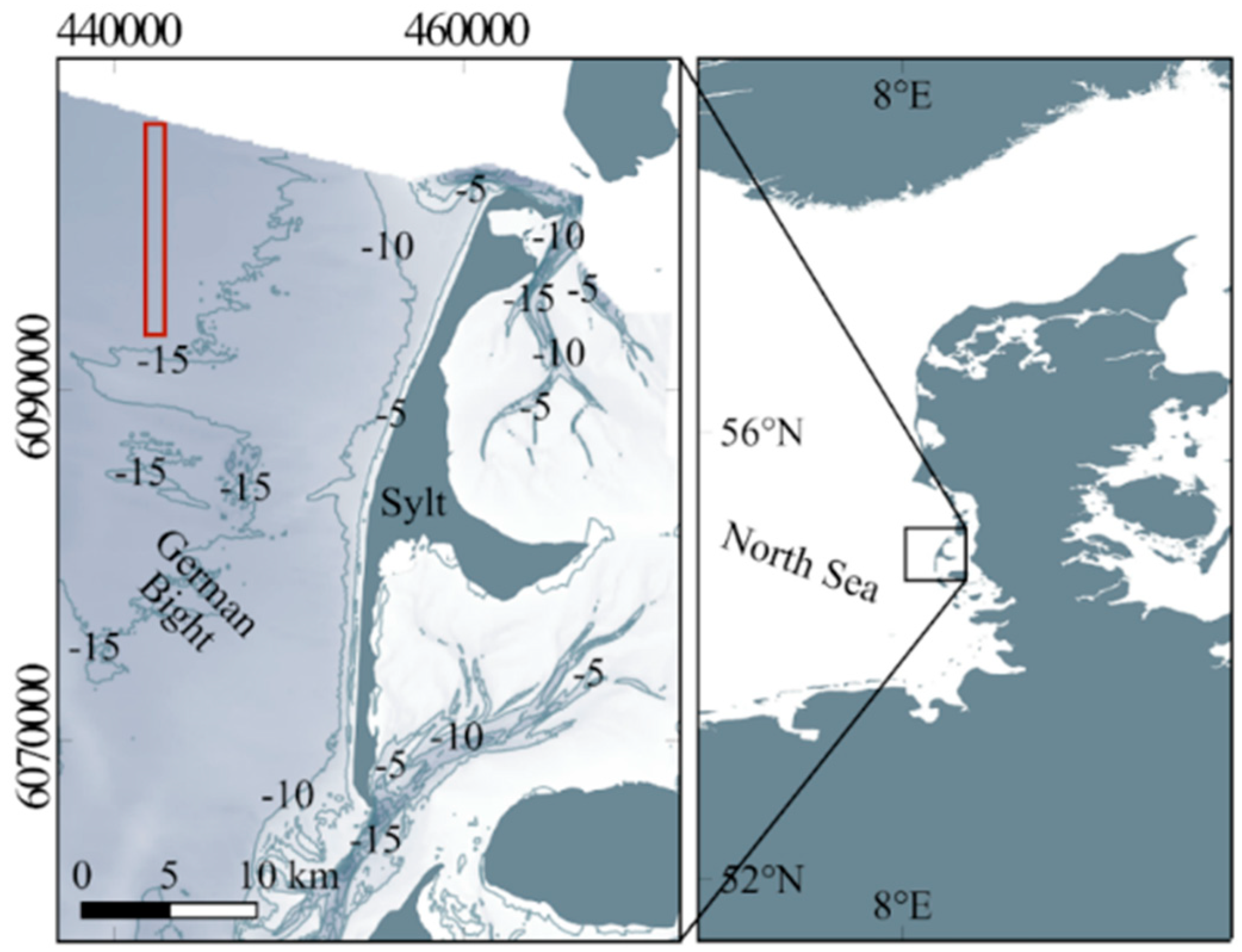
2.1. Regional Setting of the Study Area

The study site is located approx 15 km offshore the island Sylt (Figure 1) in the German Bight in water depths of 15–18 m, covering an area of 8 km2. In the area, glacial sediments of the Saalian period were covered by Weichselian periglacial and Holocene fluvial deposits [35]. These deposits were reworked during the Holocene sea level rise, leaving a low relief seafloor topography mainly composed of marine sand [36,37]. The thickness of the uppermost layer of mobile sand deposits (potentially moved by tides and storm events) reaches 1–3 m [37]. Locally, east–west directed sorted bedforms (rippled scour depressions) composed of medium to coarse sand are observed, often exposing a transgressive layer of gravel and coarse sand present at the base of the marine sands [35,36]. Sorted bedforms in the study site have a length of ~350 m and depths of 1–2 m [36]. These bedforms can remain stable over decades, although their oscillating boundaries may be covered by fine sand for varying amounts of time [36,38,39]. Reefs of the polychaete Lanice conchilega are widespread in the study site but show a high seasonal and annual change in population density [22]. The tubes of L. conchilega, formed by cemented sediment grains and shell fragments, have a diameter of up to 0.5 cm, and protrude 1–4 cm above the seafloor by [40,41]. Aggregating in patches, these reefs can have high densities of thousands of individuals per m2 and reach elevations of up to 20 cm [42].

2.2. Multibeam Echosounder

A Norbit iWBMSe multibeam echosounder mounted on the moonpool of FS Heincke was used together with an Applanix SurfMaster inertial navigation and attitude system. For the three surveys (recorded 13–16 May 2017), frequencies were set to 200, 400 and 600 kHz. EGNOS correction data were received to improve navigation to 0.5 m lateral accuracy. We registered backscatter strength using the Hypack 2016 software. Processing focused on removing the angular variations present in the data by applying an angular varied gain (AVG) and comparing relative backscatter levels between the frequencies [23]. No absolute dB values are given, as recommended by the authors of [25].
Except for frequency, the user-controllable settings of the multibeam system were kept constant and are shown in Table 1. System gains are largely removed from the multibeam output by the Norbit software (level BL1). Residual effects may still be observed because the instruments are not individually calibrated. Pulse lengths and frequencies are constant throughout the swath with no sector dependence. Backscatter data were loaded in QPS Geocoder and corrected considering survey settings and frequency-dependent absorption (Table 1). For calculation of absorption coefficients [43], the temperature was estimated as 11° with salinity to 35. AVG to flatten the backscatter mosaics was calculated using a flat seafloor assumption, given that morphological differences across the study site are minor. AVGs were averaged for complete survey lines to avoid artifacts across boundaries of changing backscatter, accepting a less ideal removal of along-track artifacts. The average seafloor response within an incidence angle interval of 30° to 60° was used to normalize the data. Beam pattern effects were removed by applying the AVG. Backscatter intensities were linearly mapped to a greyscale mosaic with a resolution of 0.3 m. The dynamic range of the mosaics is 10 dB. Dark colors represent low backscatter intensities and bright colors represent high backscatter intensities. The final mosaics were filtered using a 3 × 3 box average filter. Multi-frequency mosaics were created by using three mono-frequency greyscale mosaics as input channels of an RGB image using open source GIS software (QGIS 2.18.9, www.qgis.org). The 200 kHz frequency represents the red channel, the 400 kHz frequency the green channel, and the 600 kHz frequency the blue channel.
Angular response curves (ARCs) supporting the mosaic interpretation were calculated directly from the recorded raw data files. The angular backscatter strength is [44]:
B S ( θ ) ¯ = E L ( θ ) S L + 2 T L 10 l o g ( A ( θ ) ¯ )
where BS is the angular backscatter strength, θ is the incidence angle, EL is the recorded echo level, SL is the (estimated) source level, TL is the transmission loss (spreading + absorption) and A is the ensonified area. The calculation of the texture parameter entropy [45] supporting the mosaic interpretation was done using 32 grey levels, an inter-pixel distance of 1 and a window size of 4.5 m [46].

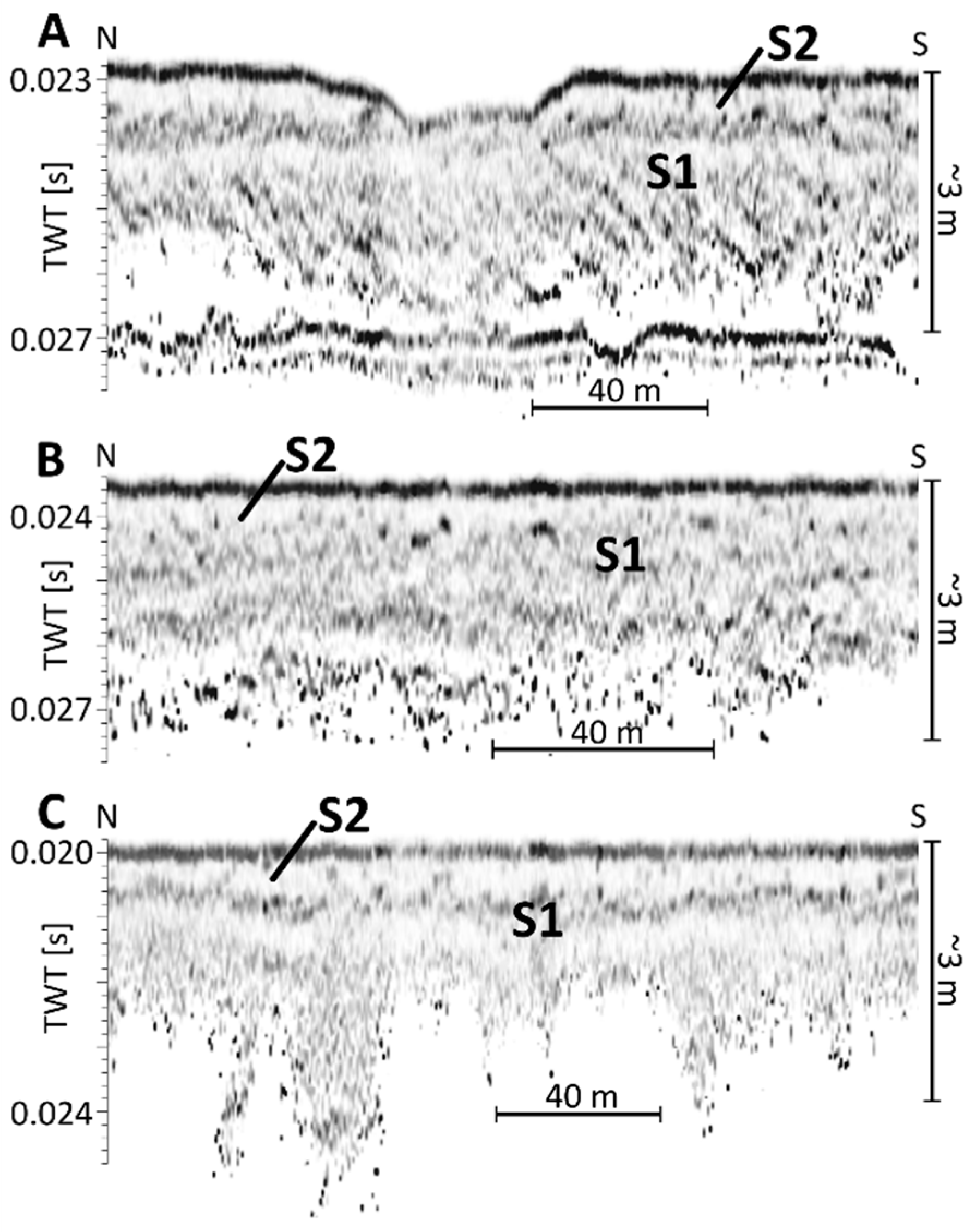
2.3. Parametric Echosounder

Supporting high-frequency seismic data were acquired using an Innomar parametric sediment echosounder to determine the shallow subsurface geology, using primary frequencies of 100 kHz and a low frequency of 12 kHz. Data were binned to 1 m intervals, and a manual time varied gain function was applied.

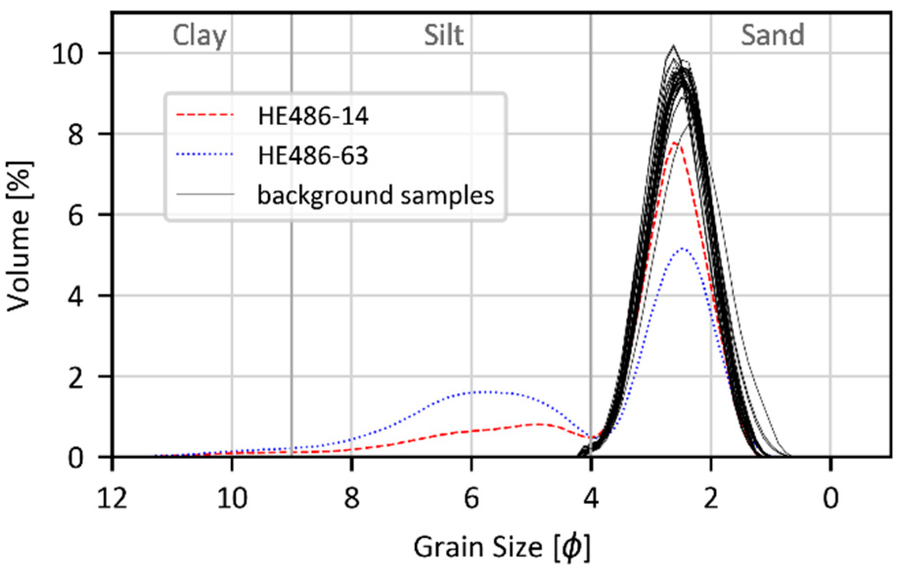
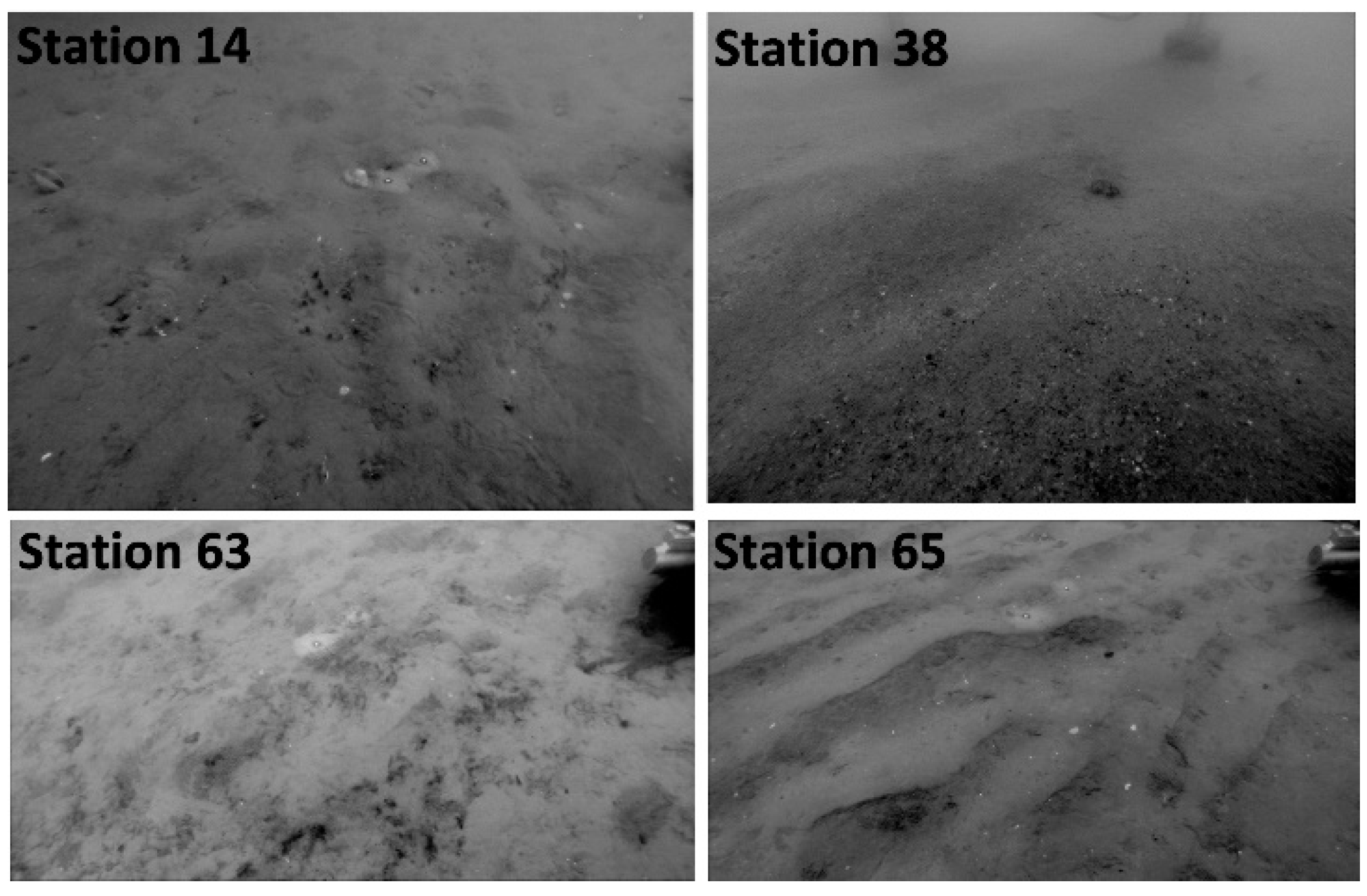
2.4. Ground Truthing
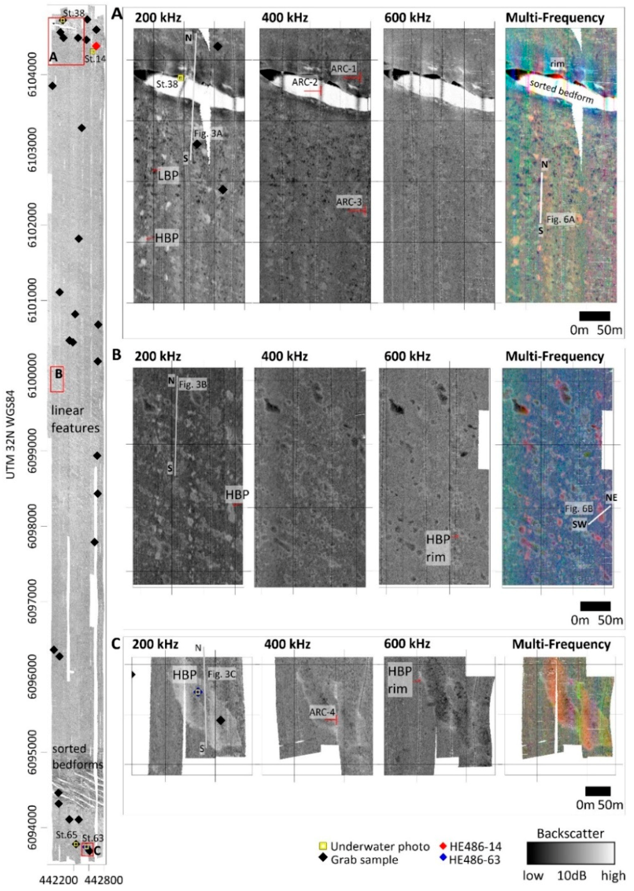
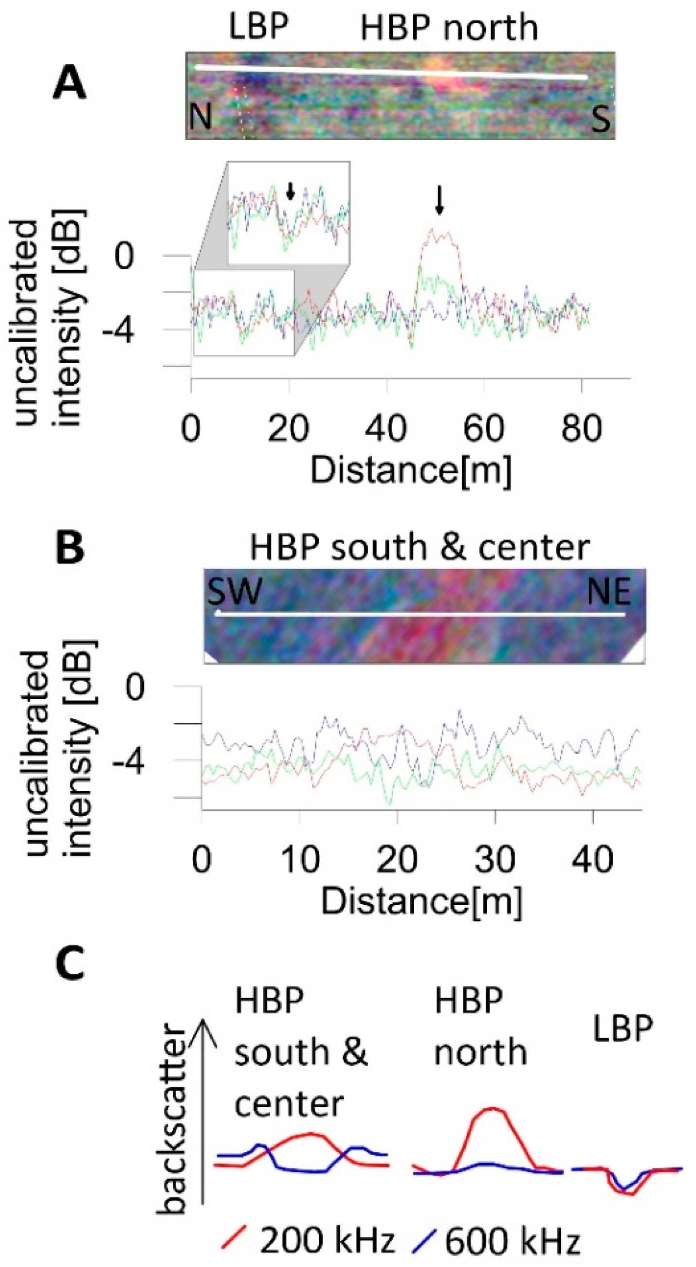
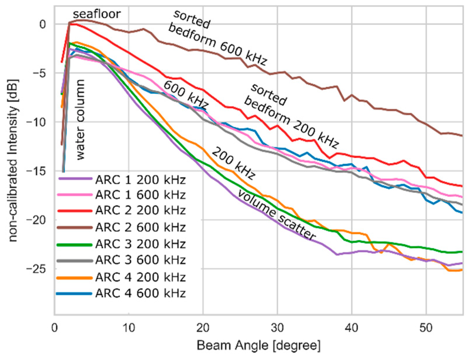
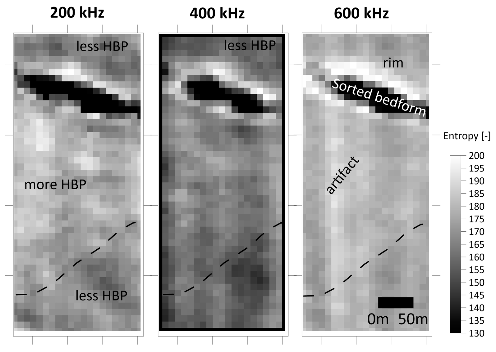
Sediment samples for ground truthing were taken using a Van-Veen type grab sampler. The generally fine-grained sediment samples were analyzed by optical grain size analysis using a CILAS 1180 particle size analyzer. Given the well-sorted sand composition with low organic content, no chemical pretreatment was applied. The mode is used as a central statistical parameter, as it is less affected by the removal of particles exceeding 1 mm in diameter. For ground truthing by underwater video, we used a Kongsberg Colour Zoom Camera (Kongsberg Maritime, Kongsberg, Norway) and a GOPRO 3+ Black Edition (GoPro, San Mateo, CA, USA) both mounted on a steel frame that was towed behind the drifting research vessel.

3. Results

Several features in backscatter mosaics (Figure 2) are frequency dependent and are described in the following. The geologic framework of these features is observed in the seismic data that shows two seismic units forming the shallow subsurface of the study site (Figure 3). Seismic unit S1 is characterized by a chaotic and inhomogeneous appearance and outcrops in the area of sorted bedforms. S1 is interpreted as the onset of a coarse sand transgression layer reported to form the sorted bedforms. Sorted bedforms are clearly detectable by morphologic depressions of 0.2–1 m (Figure 3A) and a characteristic increase in backscatter intensities. Outside of the sorted bedforms, a transparent seismic unit S2 is present (Figure 3A,C). S2 is interpreted as the layer of mobile marine sediments. Its thickness across the study site varies between 0 and approx. 1 m. The minimum thickness is observed within sorted bedforms, and a decreased thickness prevails in the central study site (Figure 3B). Outside of sorted bedforms, results of the grain size distribution suggest a homogeneous, flat seafloor composed of well-sorted fine sand with a mode around 2.5 phi (Figure 4). However, various small-scale backscatter anomalies exist. Fringing the sorted bedforms, 200 kHz data shows rims of decreased backscatter intensity aligning preferably along their northwestern edges (Figure 2A). The decrease in backscatter intensities is poorly observed in 400 kHz data, and disappears for the 600 kHz mosaic, causing a bluish north-western rim adjacent to sorted bedforms in the multi-frequency mosaic (Figure 2A).
Clearly standing out from a homogeneous background, numerous patches of increased backscatter levels (high backscatter patches, HBPs) are visually delineated. HBPs cannot be observed in bathymetric data, suggesting that the depth difference between the patches and the surrounding seafloor is less than 5 cm. In the northern part of the study site, HBPs have an irregular shape and a random distribution pattern. Their diameter is 10–25 m. In the 200 kHz mosaics, the HBPs show increased (~4 dB) backscatter intensities compared to the background sediment. The increase in intensities is reduced in the 400 kHz data (~2 dB) and hardly observed in the 600 kHz data. This results in a distinct reddish appearance of the HBP in the multi-frequency data. An increase of the silt fraction percentage is observed for sample HE486-14 retrieved from an area of densely spaced HBPs, and a poorly developed ripple pattern is recognized in nearby underwater video footage (Figure 5). An increased number of polychaetes identified as L. conchilega were observed in grab samples and underwater video images in the northern part of the investigation area, although overall observed population densities are low (Figure 5).
The shape of the HBP changes towards the south of the study site. In the central part of the study site, HBPs are aligned NW-SE parallel to the observed sorted bedforms (Figure 2). The length of the HBP differs between 5 and 70 m, while their width is approx. constant at 15 m. An intensity profile crossing an HBP (Figure 6B) reveals increased backscatter levels (~2 dB) for the low frequency. The rims of the HBPs have elevated backscatter intensities, especially in the high frequency. However, an intensity decrease to background levels or below can be observed for the inner part of the HBPs mostly at high, but sometimes also at low frequencies (Figure 2B,C). In the multi-frequency data, the HBPs have a reddish center, with bluish-greenish fringes. An example HBP with a size of ~0.013 km2 showcasing this behavior exists in the south (Figure 2C). It shows the highest backscatter intensities for the 200 kHz frequency (an increase of about 2 dB), and a reverse sensitivity with decreased backscatter intensities for the 600 kHz frequency. In the 400 kHz mosaic, only the boundaries of the HBP are recognized, while its central area is difficult to distinguish from the surrounding background sediment. Here, sample HE486-63 revealed an increased amount of silt and clay. Underwater video footage shows a weakly developed ripple pattern, black anoxic sediment directly beneath the surface and increased suspension. In contrast, video footage outside the high backscatter patch shows a distinct rippled seafloor (Figure 5).
Smaller patches of decreased backscatter levels (low backscatter patches, LBP) can be recognized in the northern study site. For LBP, backscatter levels decrease below the background fine sand intensity for all frequencies. No rim effects can be recognized. The diameter of LBP is generally smaller than 10 m. LBPs are best observed in the 200 and 400 kHz data, where the difference to the surrounding seafloor is largest (~1.5 dB). LBPs are barely visible in the 600 kHz mosaic (Figure 2), causing a dark bluish appearance in the multi-frequency mosaic.

4. Discussion

4.1. Impact of Volume Scatter

Our multi-frequency seafloor analyses show clear evidence for significantly different backscattering strengths and image textures at specific frequencies. Principally, the low frequency mosaics show the highest contrast between different seafloor facies (Figure 2), a trend that was previously noted [23]. The frequency-specific backscatter differences could be of geological or biological origin. An example of a geological cause is the increase in high-frequency scatter intensity north of the sorted bedforms. Adjacent to the sorted bedforms, oscillating boundaries to the surrounding seafloor exist, indicating the presence of a mobile fine sand layer. It is redeposited on sub-annual timescales [36] and reduces the number of scatterers in the shallow subsurface. No HBP or LBP patches are present directly at the rim in any frequency (Figure 2A), supporting a homogenous fine sand seafloor that registers with stronger backscatter intensities at higher frequencies and decreased intensities at low frequencies. Comparable trends have been previously observed in side scan sonar [31] and multibeam data [29] for sediments of low volume scatter that allow penetration of the low, but not the high frequency [30]. For sandy sediments, penetration depth is limited to ~1 cm for 600 kHz, while 200 kHz may penetrate ~8 cm into the subsurface [47].
A geologic or biologic cause of the elongated HBP in the central part of the investigation area is more difficult to establish. The HBPs may be interpreted as buried sorted bedforms covered by a thin layer of fine sand. Temporarily or completely buried sorted bedforms have been reported elsewhere [35,38]. Elevated backscatter levels are chiefly observed in the low frequency mosaics, where acoustic waves penetrated a couple of centimeters into the subsurface. A connection to sorted bedforms that could influence volume scatter by sub-bottom layering [48] is possible based on the seismic data (Figure 3B). The transparent layer (S1), interpreted as the mobile layer of fine sand [37], is of decreased thickness in the area of elongated HBPs. This indicates a thin cover of fine sand on the coarser transgressive sand layer. However, a number of factors are in contradiction to the HBP being caused by partially buried sorted bedforms. First, there is no indication of any residual depression of HBP in seismic or bathymetric data, while the active sorted bedforms in the north and south are clearly recognized by their bathymetry. Second, no coarse sand was recovered at the top or base of the grab samples taken in their vicinity, albeit Van-Veen grab samples typically recover several centimeters of sediment. Finally, angular response curves (ARCs) of the 200 kHz data (Figure 7) from the sorted bedform in the north, a mostly featureless area composed of fine sand, and different HBPs, indicate clear differences between sorted bedforms and the remaining seafloor facies. Therefore, the HBP is less likely to be of geological origin. It cannot be ruled out that geological changes in the shallow subsurface (below a few centimeters), while not significantly affecting the acoustic backscatter, impact the benthic biology of the seafloor, thus explaining the similarity in orientation between HBPs and sorted bedforms. Nevertheless, an increase in volume scatter caused by bioturbation and organic scatterers in the shallow subsurface is the most likely cause of the increased backscatter strength of the HBP at low frequencies [49]. Volume scatter is especially prevalent in silty facies [50] due to a generally decreased acoustic impedance, and generally induced by biological activity [51]. Higher frequencies capture the fine, partially silty seafloor without notable ripple features, causing a decreased backscatter intensity [30]. Under the assumption that the rims of the sorted bedforms are composed of frequently redeposited, homogeneous fine sand, ARCs (Figure 7) confirm volume scatter in the area of HBPs at incidence angles >~20°, apparent by increased scatter intensities for the 200 kHz data. No indications of volume scatter are observed in ARCs for the 600 kHz dataset. While volume scatter appears most prominent in the extended southern HBP, where an increased silt fraction is observed (ARC 4 in Figure 7), the extent of almost all HBPs is smaller than a half-swath width, which negatively affects the ability of ARCs to differentiate seafloor types. Therefore, the combined use of ARCs and multi-frequency mosaics may allow differences in volume scatter to be traced, for example, caused by the different presence of burrowing organisms and scatterers, over small scales.

4.2. Impact of Seafloor Scatter

The comparison of backscatter mosaics of different frequencies shows textural differences between HBPs in the southern/central and northern area of the study site, including the lack of a rim, the missing backscatter level inversion between high and low frequencies and a stronger and more rapid increase in backscatter levels (~4 dB in the northern versus ~2 dB in the central area). These differences could not have been observed using mono-frequency mosaics. The higher increase in backscatter levels, missing frequency inversion and comparable ARCs between HBPs in the central and northern study site indicate that volume scatter effects are not the only cause of the northern HBPs. Based on the assumption of a biologic cause of the HBPs, the tube-building species, polychaete L. conchilega is the most likely cause as it is a widespread key species in the North Sea [52] which was frequently observed in video images of the northern part of the investigation area (Figure 5), and it increases seafloor scatter [18,22]. Similar roughness-impacting organisms such as brittle star Amphiura filiformis that may reach high population densities and affect acoustic scatter [53] were not observed in high densities during the ground truthing. In the present bathymetric data, no morphology of the patches is detectable. Therefore, elevation differences in the surrounding seafloor are less than 5 cm. Since data collection took place in the beginning of May, the development of the worm aggregation after deconstruction during the winter [54] was probably in an early stage with a small number of adult individuals that are not expressed in ship-based bathymetric data. While video footage confirms the low densities of tubeworms, low population densities were found to significantly impact seafloor roughness at specific spatial wavelengths [55] and can be detected in backscatter data [16,22]. The fact that the northern HBP patches are best observed at 200 kHz is in contrast to previous findings [18] where a 445 kHz frequency was more effective than 132 kHz for the detection of L. conchilega reefs. The differences might arise due to the use of different acoustic systems (multibeam and side-scan sonar) with different footprints and pulse widths, or seasonal differences in the frequency-dependence of the backscatter strength of L. conchilega due to changing population densities. This needs to be further explored. In general, the largest impact of L. conchilega on seafloor roughness was found at spatial wavelengths of ~0.5 to 2 cm [55], where sparse L. conchilega populations increase the magnitude of seafloor roughness by up to 4 dBm4. Applying the small perturbation approximation to estimate backscatter strengths, the roughness spectrum used for the calculation of the backscatter cross section is evaluated at the Bragg wavenumber 2 k s i n ( θ ) , where k is the acoustic wavenumber and θ the incidence angle [28]. For an incidence angle of 45°, the spatial wavelengths at the Bragg wavenumber vary between 0.5 cm for 200 kHz and 0.2 cm for 600 kHz. The agreement of optical measurements of L. conchilega seafloor roughness and the frequency-dependent appearance of the northern HBP suggests that backscatter strength may be higher for lower frequencies due to changes in surface roughness caused by benthic organisms. Eventually, frequencies less than 200 kHz that were not accessible to our system would be more sensitive to tubeworm presence. Therefore, a frequency-dependent acoustic scatter may be exploited by multi-frequency surveys for benthic habitat mapping, with roughness controlled by reef density, local sediment composition, or even life cycle [21,22].
No sufficient interpretation is possible for a number of features observed in the backscatter mosaics. Several explanations are possible for the high backscatter rims observed at the boundaries of the HBP especially at higher frequencies, including either an increased surface roughness or increased presence of scatterers directly beneath the surface. However, due to the small extent of these features, a ground truthing or a detailed analysis using ARC was not possible. Similarly, the origin of the LBP observed in the northern part of the study site (Figure 2A) remains uncertain. Here, backscatter intensities decrease with increasing frequency, but are not in agreement with backscatter intensities observed for fine sand (Figure 2A, rim of the sorted bedform) or silty sediment compositions (Figure 2C). Possible explanations involve a local decrease in surface roughness (for example, due to changing grain size composition), causing locally smooth seafloor [30] combined with decreased volume scatter. However, the small extent and unsuccessful ground truthing of the LBP does not allow for a comprehensive interpretation.

4.3. Impact on Haralick Texture Parameters

Texture parameters derived from mosaics of backscatter intensity are common features for supervised or unsupervised seabed classification [56]. The acoustic frequency affects the texture parameters due to both changing survey parameters, such as footprint sizes (Table 1), but also due to the different sensitivity to seafloor features. Texture parameters derived from the backscatter mosaics in the northern part of the study site show that the different sensitivity of the mono-frequency mosaics to seafloor features carries over to derived textural parameters. Maps of seafloor entropy (Figure 8), a parameter that is closely correlated with homogeneity and contrast in sedimentary facies [46], demonstrate that the increased density of HBP and LBP in the northern part of the study site is best captured at low and medium frequencies, supporting the sensitivity of texture parameters to the presence of benthic organisms [22].

5. Conclusions

For sediment classification including the recognition of benthic habitats, backscatter data of lower frequencies (200 kHz) showed an increased sensitivity to changes in seafloor composition in a sedimentary continental shelf setting. It is suggested that low frequencies be incorporated in mapping programs utilizing backscatter information. The consideration of multiple frequencies allowed an improved interpretation of subtle seafloor features, although the limited availability of calibrated multi-frequency multibeam echosounders hindered quantitative data interpretation. The application of multi-frequency mosaics is especially promising for the detection of benthic life, which may vary over scales not accessible to interpretation by backscatter angular response curves or routine ground truthing. Introducing multispectral data increases data dimensionality, and may lend itself to automated seafloor classification. However, our results show that for practical application of multi-frequency data for habitat mapping, we lack the information to interpret many backscatter features of the seafloor. Therefore, the concurrent recording of calibrated multi-frequency backscatter data and precisely positioned geological and biological ground truthing, including the shallow subsurface, are required to establish interrelationships and fully utilize the potential of modern multibeam echosounders in the future.

Author Contributions

Conceptualization, P.F. and S.P.; Formal analysis, P.F., I.S. and S.P.; Funding acquisition, P.F. and J.S.v.D.; Investigation, P.F., I.S., S.P., M.S. and J.S.v.D.; Methodology, P.F. and I.S.; Project administration, P.F. and J.S.v.D.; Writing—original draft, P.F. and I.S.; Writing—review and editing, S.P., M.S. and J.S.v.D.

Funding

Part of this work resulted from the BONUS ECOMAP project, supported by BONUS (Art 185), funded jointly by the EU and the Federal Ministry of Education and Research of Germany (BMBF), the National Centre for Research and Development of Poland (NCBR), and the Innovation Fund Denmark (Innovationsfonden).

Acknowledgments

We thank the master and crew of FS Heincke for their support during our research survey HE486. We thank Philipp Held, Dennis Wilken, Arne Lohrberg and our student assistants for their help during the survey. The helpful and constructive comments of three anonymous reviewers improved the manuscript.

Conflicts of Interest

The authors declare no conflict of interest.

Data Availability

Raw multibeam echosounder data and underwater videos of FS Heincke survey 486 are stored on dedicated servers of the Leibniz Institute for Baltic Sea Research Warnemünde and are available upon request.

References

  1. Anderson, J.T.; Van Holliday, D.; Kloser, R.; Reid, D.G.; Simard, Y. Acoustic seabed classification: Current practice and future directions. ICES J. Mar. Sci. 2008, 65, 1004–1011. [Google Scholar] [CrossRef]
  2. Brown, C.J.; Blondel, P. Developments in the application of multibeam sonar backscatter for seafloor habitat mapping. Appl. Acoust. 2009, 70, 1242–1247. [Google Scholar] [CrossRef]
  3. Jackson, D.R.; Winebrenner, D.P.; Ishimaru, A. Application of the composite roughness model to high-frequency bottom backscattering. J. Acoust. Soc. Am. 1986, 79, 1410–1422. [Google Scholar] [CrossRef]
  4. Lamarche, G.; Lurton, X.; Verdier, A.-L.; Augustin, J.-M. Quantitative characterisation of seafloor substrate and bedforms using advanced processing of multibeam backscatter—Application to Cook Strait, New Zealand. Cont. Shelf Res. 2011, 31, S93–S109. [Google Scholar] [CrossRef]
  5. Yu, J.; Henrys, S.A.; Brown, C.; Marsh, I.; Duffy, G. A combined boundary integral and Lambert’s Law method for modelling multibeam backscatter data from the seafloor. Cont. Shelf Res. 2015, 103, 60–69. [Google Scholar] [CrossRef]
  6. Sternlicht, D.D.; de Moustier, C.P. Time-dependent seafloor acoustic backscatter (10–100 kHz). J. Acoust. Soc. Am. 2003, 114, 2709–2725. [Google Scholar] [CrossRef] [PubMed]
  7. Fonseca, L.; Brown, C.; Calder, B.; Mayer, L.; Rzhanov, Y. Angular range analysis of acoustic themes from Stanton Banks Ireland: A link between visual interpretation and multibeam echosounder angular signatures. Appl. Acoust. 2009, 70, 1298–1304. [Google Scholar] [CrossRef]
  8. Rzhanov, Y.; Fonseca, L.; Mayer, L. Construction of seafloor thematic maps from multibeam acoustic backscatter angular response data. Comput. Geosci. J. 2012, 41, 181–187. [Google Scholar] [CrossRef]
  9. Stephens, D.; Diesing, M. Towards quantitative spatial models of seabed sediment composition. PLoS ONE 2015, 10, e0142502. [Google Scholar] [CrossRef] [PubMed] [Green Version]
  10. Foote, K.G.; Aglen, A.; Nakken, O. Measurement of fish target strength with a split-beam echo sounder. J. Acoust. Soc. Am. 1986, 80, 612–621. [Google Scholar] [CrossRef] [Green Version]
  11. Hashim, M.; Aziz, M.F.; Hassan, R.B.; Hossain, M.S. Assessing target strength, abundance, and biomass for three commercial pelagic fish species along the East coast of Peninsular Malaysia using a Split-Beam echo sounder. J. Coast. Res. 2017, 33, 1448–1459. [Google Scholar] [CrossRef]
  12. Roberts, J.M.; Brown, C.J.; Long, D.; Bates, C.R. Acoustic mapping using a multibeam echosounder reveals cold-water coral reefs and surrounding habitats. Coral Reefs 2005, 24, 654–669. [Google Scholar] [CrossRef]
  13. Huehnerbach, V.; Blondel, P.; Huvenne, V.; Freiwald, A. Habitat mapping on a deep-water coral reef off Norway, with a comparison of visual and computer-assisted sonar imagery interpretation. In Mapping the Seafloor for Habitat Characterization; Todd, B., Greene, G., Eds.; Geological Association of Canada: St. John’s, NL, Canada, 2007; p. 12. [Google Scholar]
  14. Glogowski, S.; Dullo, W.-C.; Feldens, P.; Liebetrau, V.; von Reumont, J.; Hühnerbach, V.; Krastel, S.; Wynn, R.B.; Flögel, S. The Eugen Seibold coral mounds offshore western Morocco: Oceanographic and bathymetric boundary conditions of a newly discovered cold-water coral province. Geo-Mar. Lett. 2015, 35, 257–269. [Google Scholar] [CrossRef]
  15. Kostylev, V.; Todd, B.; Fader, G.; Courtney, R.; Cameron, G.; Pickrill, R. Benthic habitat mapping on the Scotian Shelf based on multibeam bathymetry, surficial geology and sea floor photographs. Mar. Ecol. Prog. Ser. 2001, 219, 121–137. [Google Scholar] [CrossRef] [Green Version]
  16. Self, R.F.L.; A’Hearn, P.; Jumars, P.A.; Jackson, D.R.; Richardson, M.D.; Briggs, K.B. Effects of macrofauna on acoustic backscatter from the seabed: Field manipulations in West Sound, Orcas Island, Washington, U.S.A. J. Mar. Res. 2001, 59, 991–1020. [Google Scholar] [CrossRef]
  17. Brown, C.; Hewer, A.; Limpenny, D.; Cooper, K.; Rees, H.; Meadows, W. Mapping seabed biotopes using sidescan sonar in regions of heterogeneous substrata: Case study east of the Isle of Wight, English Channel. Underw. Technol. Int. J. Soc. Underw. 2004, 26, 27–36. [Google Scholar] [CrossRef]
  18. Degraer, S.; Moerkerke, G.; Rabaut, M.; Van Hoey, G.; Du Four, I.; Vincx, M.; Henriet, J.-P.; Van Lancker, V. Very-high resolution side-scan sonar mapping of biogenic reefs of the tube-worm Lanice conchilega. Remote Sens. Environ. 2008, 112, 3323–3328. [Google Scholar] [CrossRef]
  19. McGonigle, C.; Brown, C.; Quinn, R.; Grabowski, J. Evaluation of image-based multibeam sonar backscatter classification for benthic habitat discrimination and mapping at Stanton Banks, UK. Estuar. Coast. Shelf Sci. 2009, 81, 423–437. [Google Scholar] [CrossRef]
  20. De Falco, G.; Tonielli, R.; Di Martino, G.; Innangi, S.; Simeone, S.; Michael Parnum, I. Relationships between multibeam backscatter, sediment grain size and Posidonia oceanica seagrass distribution. Cont. Shelf Res. 2010, 30, 1941–1950. [Google Scholar] [CrossRef]
  21. Raineault, N.; Trembanis, A.C.; Miller, D.C. Mapping benthic habitats in Delaware Bay and the coastal Atlantic: acoustic techniques provide greater coverage and high resolution in complex, shallow-water environments. Estuar. Coasts 2012, 35, 682–699. [Google Scholar] [CrossRef]
  22. Heinrich, C.; Feldens, P.; Schwarzer, K. Highly dynamic biological seabed alterations revealed by side scan sonar tracking of Lanice conchilega beds offshore the island of Sylt (German Bight). Geo-Mar. Lett. 2017, 37, 289–303. [Google Scholar] [CrossRef]
  23. Clarke, J.E.H. Multispectral acoustic backscatter from Multibeam, improved classification potential. In Proceedings of the United States Hydrographic Conference, San Diego, CA, USA, 15–19 March 2015. [Google Scholar]
  24. Tamsett, D.; McIlvenny, J.; Watts, A. Colour sonar: Multi-frequency sidescan sonar images of the seabed in the Inner Sound of the Pentland Firth, Scotland. J. Mar. Sci. Eng. 2016, 4, 26. [Google Scholar] [CrossRef]
  25. Lamarche, G.; Lurton, X. Recommendations for improved and coherent acquisition and processing of backscatter data from seafloor-mapping sonars. Mar. Geophys. Res. 2017. [CrossRef]
  26. Williams, K.L.; Jackson, D.R.; Thorsos, E.I.; Tang, D.; Schock, S.G. Comparison of sound speed and attenuation measured in a sandy sediment to predictions based on the Biot theory of porous media. IEEE J. Ocean. Eng. 2002, 27, 413–428. [Google Scholar] [CrossRef]
  27. Williams, K.L.; Jackson, D.R.; Tang, D.; Briggs, K.B.; Thorsos, E.I. Acoustic backscattering from a sand and a sand/mud environment: Experiments and data/model comparisons. IEEE J. Ocean. Eng. 2009, 34, 388–398. [Google Scholar] [CrossRef]
  28. Lamarche, G.; Lurton, X. Backscatter Measurements by Seafloor-Mapping Sonars. Guidelines and Recommendations. Available online: http://geohab.org/wp-content/uploads/2013/02/BWSG-REPORT-MAY2015.pdf (accessed on 11 June 2018).
  29. Clarke, J.E.H.; Iwanowska, K.K.; Parrott, R.; Duffy, G.; Lamplugh, M.; Griffin, J. Inter-calibrating multi-source, multi-platform backscatter data sets to assist in compiling regional sediment type maps: Bay of Fundy. In Proceedings of the Joint Canadian Hydrographic and National Surveyors’ Conference, Victoria, Australia, 26–29 March 2008; pp. 1–22. [Google Scholar]
  30. Ryan, W.B.F.; Flood, R.D. Side-looking sonar backscatter response at dual frequencies. Mar. Geophys. Res. 1996, 18, 689–705. [Google Scholar] [CrossRef]
  31. Tauber, F. Search for paleo-landscapes in the southwestern Baltic Sea with sidescan sonar. Ber. RGK 2011, 92, 323–349. [Google Scholar]
  32. Collier, J.S.; Brown, C.J. Correlation of sidescan backscatter with grain size distribution of surficial seabed sediments. Mar. Geol. 2005, 214, 431–449. [Google Scholar] [CrossRef]
  33. Klaucke, I.; Weinrebe, W.; Petersen, C.J.; Bowden, D. Temporal variability of gas seeps offshore New Zealand: Multi-frequency geoacoustic imaging of the Wairarapa area, Hikurangi margin. Mar. Geol. 2010, 272, 49–58. [Google Scholar] [CrossRef] [Green Version]
  34. Schneider von Deimling, J.; Weinrebe, W.; Tóth, Z.; Fossing, H.; Endler, R.; Rehder, G.; Spieß, V. A low frequency multibeam assessment: Spatial mapping of shallow gas by enhanced penetration and angular response anomaly. Mar. Pet. Geol. 2013, 44, 217–222. [Google Scholar] [CrossRef] [Green Version]
  35. Diesing, M.; Kubicki, A.; Winter, C.; Schwarzer, K. Decadal scale stability of sorted bedforms, German Bight, southeastern North Sea. Cont. Shelf Res. 2006, 26, 902–916. [Google Scholar] [CrossRef]
  36. Mielck, F.; Holler, P.; Bürk, D.; Hass, H.C. Interannual variability of sorted bedforms in the coastal German Bight (SE North Sea). Cont. Shelf Res. 2015, 111, 31–41. [Google Scholar] [CrossRef]
  37. Zeiler, M.; Schulz-Ohlberg, J.; Figge, K. Mobile sand deposits and shoreface sediment dynamics in the inner German Bight (North Sea). Mar. Geol. 2000, 170, 363–380. [Google Scholar] [CrossRef]
  38. Thieler, E.R.; Pilkey, O.H.; Cleary, W.J.; Schwab, W.C. Modern sedimentation on the shoreface and inner continental shelf at Wrightsville Beach, North Carolina, USA. J. Sediment. Res. 2001, 71, 958–970. [Google Scholar] [CrossRef]
  39. Murray, A.B.; Thieler, E.R. A new hypothesis and exploratory model for the formation of large-scale inner-shelf sediment sorting and “rippled scour depressions”. Cont. Shelf Res. 2004, 24, 295–315. [Google Scholar] [CrossRef]
  40. Ziegelmeier, E. Beobachtungen über den Röhrenbau von Lanice conchilega (Pallas) im Experiment und am natürlichen Standort. Helgolander Wiss. Meeresunters 1952, 4, 107–129. [Google Scholar] [CrossRef]
  41. Callaway, R. Juveniles stick to adults: Recruitment of the tube-dwelling polychaete Lanice conchilega (Pallas, 1766). Hydrobiologia 2003, 503, 121–130. [Google Scholar] [CrossRef]
  42. Rabaut, M.; Vincx, M.; Degraer, S. Do Lanice conchilega (sandmason) aggregations classify as reefs? Quantifying habitat modifying effects. Helgol. Mar. Res. 2009, 63, 37–46. [Google Scholar] [CrossRef]
  43. Ainslie, M.A.; McColm, J.G. A simplified formula for viscous and chemical absorption in sea water. J. Acoust. Soc. Am. 1998, 103, 1671–1672. [Google Scholar] [CrossRef]
  44. Hellequin, L.; Boucher, J.M.; Lurton, X. Processing of high-frequency multibeam echo sounder data for seafloor characterization. IEEE J. Ocean. Eng. 2003, 28, 78–89. [Google Scholar] [CrossRef]
  45. Haralick, R.M.; Shanmugam, K.; Dinstein, I. Textural Features for Image Classification. IEEE Trans. Syst. Man Cybern. 1973, 6, 610–621. [Google Scholar] [CrossRef]
  46. Feldens, P. Sensitivity of texture parameters to acoustic incidence angle in multibeam backscatter. IEEE Geosci. Remote Sens. Lett. 2017, 14, 2215–2219. [Google Scholar] [CrossRef]
  47. Huff, L.C. Acoustic Remote Sensing as a Tool for Habitat Mapping in Alaska Waters. In Marine Habitat Mapping Technology for Alaska; Reynolds, J.R., Greene, H.G., Eds.; Alaska Sea Grant, University of Alaska Fairbanks: Fairbanks, AK, USA, 2008; pp. 29–46. [Google Scholar]
  48. Schneider von Deimling, J.; Held, P.; Feldens, P.; Wilken, D. Effects of using inclined parametric echosounding on sub-bottom acoustic imaging and advances in buried object detection. Geo-Mar. Lett. 2016, 36, 113–119. [Google Scholar] [CrossRef] [Green Version]
  49. Urgeles, R.; Locat, J.; Schmitt, T.; Hughes Clarke, J.E. The July 1996 flood deposit in the Saguenay Fjord, Quebec, Canada: Implications for sources of spatial and temporal backscatter variations. Mar. Geol. 2002, 184, 41–60. [Google Scholar] [CrossRef]
  50. Jackson, D.R.; Briggs, K.B. High-frequency bottom backscattering: Roughness versus sediment volume scattering. J. Acoust. Soc. Am. 1992, 92, 962–977. [Google Scholar] [CrossRef]
  51. Jensen, F.B.; Kuperman, W.A.; Porter, M.B.; Schmidt, H. Computational Ocean Acoustics; Springer Science & Business Media: Berlin, Germany, 2011; ISBN 9781441986788. [Google Scholar]
  52. Van Hoey, G.; Guilini, K.; Rabaut, M.; Vincx, M.; Degraer, S. Ecological implications of the presence of the tube-building polychaete Lanice conchilega on soft-bottom benthic ecosystems. Mar. Biol. 2008, 154, 1009–1019. [Google Scholar] [CrossRef]
  53. Hass, H.C.; Mielck, F.; Fiorentino, D.; Papenmeier, S.; Holler, P.; Bartholomä, A. Seafloor monitoring west of Helgoland (German Bight, North Sea) using the acoustic ground discrimination system RoxAnn. Geo-Mar. Lett. 2017, 37, 125–136. [Google Scholar] [CrossRef]
  54. Carey, D. Sedimentological effects and palaeoecological implications of the tube-building polychaete Lanice conchilega Pallas. Sedimentology 1987, 34, 49–66. [Google Scholar] [CrossRef]
  55. Schönke, M.; Feldens, P.; Wilken, D.; Papenmeier, S.; Heinrich, C.; Schneider von Deimling, J.; Held, P.; Krastel, S. Impact of Lanice conchilega on seafloor microtopography off the island of Sylt (German Bight, SE North Sea). Geo-Mar. Lett. 2017, 37, 305–318. [Google Scholar] [CrossRef]
  56. Blondel, P.; Gómez Sichi, O. Textural analyses of multibeam sonar imagery from Stanton Banks, Northern Ireland continental shelf. Appl. Acoust. 2009, 70, 1288–1297. [Google Scholar] [CrossRef]
Figure 1. Location of the study site in the North Sea, marked with a red rectangle. Bathymetric data is derived from the BSH GeoSeaPortal (www.geoseaportal.de). Coordinates of the inset are in UTM32N WGS84.
Geosciences 08 00214 g001
Figure 2. Backscatter data recorded in the study site. The overview image to the left shows the available data and position of the insets (AC). The overview mosaic was contrast-stretched. Insets (A), (B) and (C) show mosaics of 200, 400 and 600 kHz and an RGB multi-frequency mosaic for selected areas. Examples of high backscatter patches (HBP) and low backscatter patches (LBP) are annotated. The position of seismic lines (Figure 3), grab samples (Figure 4), underwater video (Figure 5), cross sections through the multi-frequency mosaic (Figure 6), and angular response curves (ARC, Figure 7) is indicated.
Geosciences 08 00214 g002
Figure 3. Seismic data reveals the geological structure of the shallow subsurface in the northern (A), central (B) and southern part (C) of the investigated area. A transparent layer composed of fine sand (S2) is observed above a coarse sand transgression layer (S1). Refer to Figure 2 for position of the seismic lines.
Geosciences 08 00214 g003
Figure 4. Grain size composition in the study site. The majority of the samples have a well-sorted fine sand composition. The position of two samples with increased silt content is marked in Figure 2.
Geosciences 08 00214 g004
Figure 5. Underwater video footage from the northern study site (station 14) shows small numbers of L. conchilega tubeworms. In contrast, station 38 at the boundary of a sorted bedform comprises rippled coarse sand. In the south, station 63 shows different benthic assemblages in the center of a high backscatter patch. Outside of the patch, a clear ripple pattern prevails (station 65). Refer to Figure 2 for positions.
Geosciences 08 00214 g005
Figure 6. The cross sections (A) and (B) through the multi-frequency mosaic showcase the frequency-dependent response of high backscatter patches (HBP) and low backscatter patches (LBP). Refer to Figure 2 for the position of the cross sections. (C) displays the schematic of the different observed backscatter anomalies.
Geosciences 08 00214 g006
Figure 7. Angular response curves at the rim (ARC 1) and within (ARC 2) a sorted bedform, in the area of densely spaced HBP (ARC 3) in the northern study site and across a large HBP in the southern study site (ARC 4). The shape of the ARC within a sorted bedform differs clearly from all other sediments. Indications of volume scatter at >20° incidence angle are only observed in the 200 kHz dataset. Refer to Figure 2 for position.
Geosciences 08 00214 g007
Figure 8. Texture parameter entropy for the northern region of the study site, corresponding to Figure 2A. It can be observed that the boundary between the density of less and more high backscatter patches (HBP) is more clearly observed in the 200 kHz data, while the boundary fringing the sorted bedforms is better observed in 600 kHz data. The presence of along-track artifacts is amplified in the texture images.
Geosciences 08 00214 g008
Table 1. Multibeam echosounder settings during data acquisition. Multiple values correspond to frequencies of 200, 400 and 600 kHz respectively. Source levels of the 200 and 600 kHz frequency are unknown.
ParameterValueParameterValue
Bandwidth chirp (kHz)80 Spreading0
Chirp pulse length (ms)0.2 Absorption (dB/km)0
Center frequency (kHz)200/400/600 Static gain (dB)0
Across track beam width at center frequency (°)1.8/0.9/0.6Along-track beam width at center frequency (°)3.8/1.9/1.3
Absorption coefficient (dB/km)60/100/170Source level (dB re µPa)-/227/-

