Correlation Analysis of Seasonal Temperature and Precipitation in a Region of Southern Italy


1
Department of Computer Engineering, Modeling, Electronics, and Systems Science (DIMES), University of Calabria, 87036 Rende (CS), Italy
2
Research Institute for Geo-hydrological Protection (CNR-IRPI), National Research Council of Italy, 87036 Rende (CS), Italy
3
Department of Environmental and Chemical Engineering (DIATIC), University of Calabria, 87036 Rende (CS), Italy
*
Author to whom correspondence should be addressed.
Geosciences 2018, 8(5), 160; https://doi.org/10.3390/geosciences8050160
Submission received: 27 March 2018
/
Revised: 27 April 2018
/
Accepted: 28 April 2018
/
Published: 2 May 2018
(This article belongs to the Special Issue Hydrological Hazard: Analysis and Prevention)
Abstract
:The investigation of the statistical links between changes in temperature and rainfall, though not widely achieved in the past, is an interesting issue because their physical interdependence is difficult to point out. Aiming at detecting possible trends with a pooled approach, a correlative analysis of temperature and rainfall has been carried out by comparing changes in their standardized anomalies from two different 30-year time periods. The procedure has been applied to the time series of seasonal mean temperature and cumulative rainfall observed in four sites of the Calabria region (Southern Italy), with reference to the series which verify the normality hypothesis. Specifically, the displacements of the ellipses, representing the probability density functions of the bivariate normal distribution assumed for the climatic variables, have been quantified and tested for each season, passing from the first subperiod to the following one. The main results concern a decreasing trend of both the temperature and the rainfall anomalies, predominantly in the winter and autumn seasons.
1. Introduction
Rainfall and air temperature are among the most investigated meteorological variables in climatic trend studies, mainly due to the serious implications that their spatial and temporal changes can have on several environmental and socioeconomic aspects [1,2,3]. With regard to the temporal distribution of rainfall, long-term trends have been detected in several areas of the world [4,5]. In the Mediterranean Basin, an alternation of extreme rainy periods and severe droughts or water shortages has been detected [6]. Furthermore, this area is characterized by significant rainfall variability [7,8], caused by synoptic dynamics of extreme events evolving along this basin [9].
In Italy, which has a central position in the Mediterranean area, investigations of long rainfall series showed a decreasing trend, even if not always significant [10]. More detailed analyses have been carried out at smaller scales with varied behaviour: decreasing rainfall amounts in winter versus precipitation increase in the summer months. In particular, these behaviours were detected in the regions of Southern Italy, such as Campania [11], Basilicata [12], Sicily [13], and Calabria [14].
Regarding temperature, several studies evidenced the increase of the mean values of temperatures both at large [15] and local spatial scales [16]. The magnitude of trends varies according to the study area and the studied period. In addition, the increasing rates of maximum and minimum temperatures present a high variability. In the last decades, the analyses of temperature have been focused on the extreme values [17,18]. Salinger and Griffiths [19] showed that the changes in mean and extreme values are closely interconnected between each other and that low trends in average conditions can generate high variations in the extremes, especially in their frequency. Donat and Alexander [20] showed that both daytime (daily maximum) and night-time (daily minimum) temperatures have become higher over the past 60 years, but at different rates: greater for minimum than for maximum values. In Italy, which can be considered as a climate change hotspot [21], variations in the probability density functions of the minimum and maximum daily temperature anomalies were studied by Simolo et al. [22]. Caloiero et al. [23] analysed the minimum and maximum monthly temperatures of 19 stations in Calabria and detected a positive trend for spring and summer months and a marked negative one in September.
In fact, an accurate joint analysis of precipitation and temperature is more difficult to be carried out because of the possible interdependence between them [24]. Nevertheless, Rajeevan et al. [25] found that temperature and rainfall in India were positively correlated during January and May, but negatively correlated during July. Huang et al. [26] showed a negative correlation between rainfall and temperature in the Yellow River basin of China. Cong and Brady [27] applied the copula models to the rainfall and temperature data of a province of Sweden, and they evidenced negative correlations in the months from April to July and in September. Caloiero et al. [14] analysed the spatial and temporal behaviour of monthly precipitation and temperature in the Calabria region (Southern Italy), comparing the Péguy climographs [28] on three subperiods of the whole observation period (1916–2010).
In this paper, a joint analysis of temperature and rainfall has been carried out, comparing time series recorded in some gauges located in Calabria (Southern Italy) over two distinct 30-year subperiods (1951–1980 and 1981–2010). In particular, the anomalies of the seasonal values of temperature and precipitation, standardized by means of the mean values and the standard deviations of the period 1961–1990, were analysed. The series have been selected based on the normality hypothesis. The isocontour lines of the probability density function for the bivariate Gaussian distribution have been considered as ellipses centred on the vector mean of each subperiods. Finally, some statistical tests were applied for verifying the variations of these ellipses passing from one subperiod to the other, aiming at detecting joint trends of the seasonal temperature and rainfall anomalies.
2. Materials and Methods
2.1. Study Area and Data
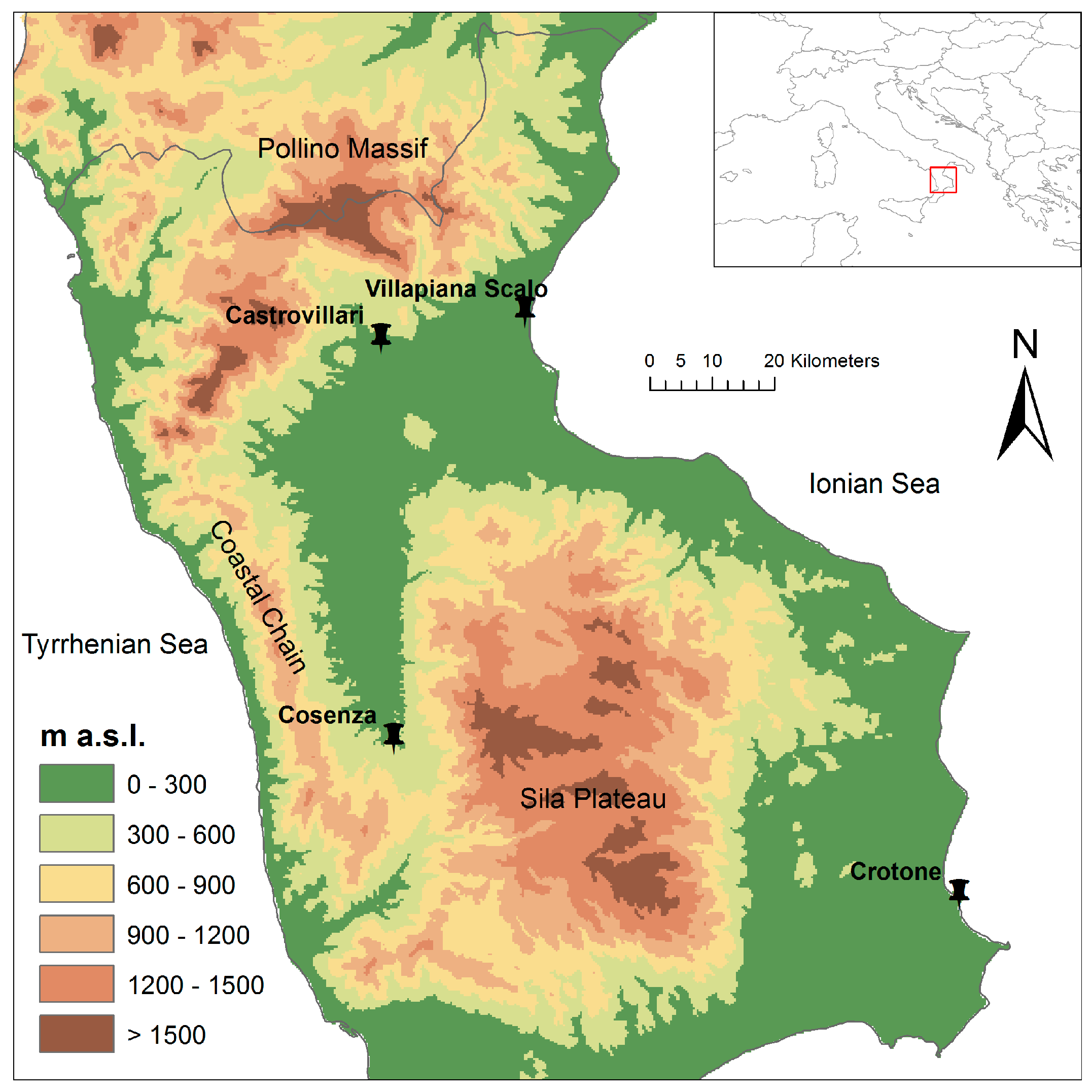
Calabria is situated in the southern part of the Italian peninsula, with an area of 15,080 km2 and a perimeter of about 818 km (Figure 1). This region shows high climatic contrasts, due to the geographic position and mountainous nature. Its climate is characterized by typical subtropical summers, with colder snowy winters and fresher summers in the inland zones, typical of Mediterranean areas. Its elongated shape evidences two coastal sides with dissimilar climatic features. The Ionian coast is exposed to the warm African currents, thus experiencing high temperatures with short and heavy precipitation. In contrast, the Tyrrhenian side is more influenced by Western air currents, which cause milder temperatures and orographic precipitation.
The climatic database used in this study, managed by the former Italian Hydrographic Service, concerns the monthly values of cumulated rainfall and mean temperature of some stations characterizing the different climatic conditions of the region for the period 1951–2010. Particular attention has been given to the problems arising from the low quality and inhomogeneities of the data series. Specifically, the monthly database was a part of the high-quality one presented in a previous study, which detected the inhomogeneities through a multiple application of the Craddock test [29]. In particular, four homogeneous monthly cumulated rainfall and mean temperature series were selected, whose percentages of missing data are presented in Table 1. The main statistical features of the seasonal temperature and rainfall series for the reference period 1961–1990 are shown in Table 2.
2.2. Methods
The statistical approach here used to explore the relationships between climatic data series which are not perfectly similar, such as monthly rainfall and temperature, is the correlative analysis applied to the standardized anomalies [30]. This approach also allows for the comparisons of data series of different time periods and lengths [31]. The standardized anomalies of seasonal values of temperature and rainfall were calculated for each site by using their means and standard deviations calculated for the reference period 1961–1990. In this way, the origin of the temperature versus precipitation plots shown in this study corresponds to the mean values of this reference time span, while the anomalies of the two variables extend over the four quadrants of the plot. Specifically, the peculiar climatic conditions of each quadrant are: warm and wet for the upper right quadrant, cold and wet for the upper left one, cold and dry for the lower left one, and warm and dry for the lower right quadrant.
Previous studies on the long-term cumulated rainfall in the Calabria region indicated a shift towards drier conditions around the year 1980 [32,33]. Thus, in order to search for possible temporal trends, the whole 1951–2010 time interval of the data set was fragmented into two 30-year periods: 1951–1980 and 1981–2010. The normality hypothesis was separately tested for both the variables and the 30-year periods by means of the Anderson–Darling test [34]. This is a goodness-of-fit test specially devised to give heavier weights to the distribution tails (where outliers are sometimes located) than the Kolmogorov–Smirnov test.
Only in the cases where the normality hypothesis was not rejected, the correlation analysis has been successively performed. In particular, a bivariate Gaussian distribution was applied to the seasonal variables in each site for the two 30-year periods separately. The probability density function of this distribution can be visualized as isocontour lines in the temperature–rainfall (T–R) plane with prefixed significance levels αi. These lines are (1−αi)% confidence ellipses centered on the mean values of the variables. In this study, the significance level has been fixed as equal to 0.05, thus characterizing each correlation by means of a 95% confidence ellipse, which is oriented according to the sign of its correlation coefficient [31].
Each ellipse can be described through the vector of the means and the variance–covariance matrix, while its eigenvectors provide the directions of its major and minor axes. If the variables show changes between the two subperiods, the results are displacements of the ellipses in the T–R plane, generally formed by rigid transformations (translations and/or rotations) and deformations of the ellipses. Specifically, the translation concerns a modification in the means vector of the ellipses, and the rotation is due to variations in the correlation coefficients, while the deformation is linked to a change in the variance–covariance matrix.
All these cases can be verified through the application of specific statistical tests. In particular, the global statistical significance of the change in the means vector (, ) can be assessed through the multivariate Hotelling’s test [35], while the statistical significance of the change of each single value of the vector can be verified by means of the univariate t-test of difference in the mean [30].
Concerning the orientation of the ellipses, the statistical significance of the difference in the correlation coefficients passing from a subperiod to the other one can be tested by preliminarily transforming each correlation coefficient between the seasonal temperature and the rainfall anomalies, ρ, into z score through the Fisher Z-transformation [30]:
In this way, firstly, the Z value obtained for each subperiod can be used to test the significance of its correlation coefficient, given that Z is approximately distributed as a normal law with μ = 0 and σ = (N − 3)−0.5, where N is the length of the anomalies series. Then, the difference in the correlation coefficients can be tested through the bivariate test statistic:
which combines the Z1 and Z2 values evaluated for the correlation coefficients ρ1 and ρ2 of the two subperiods 1951–1980 and 1981–2010 with lengths N1 and N2, respectively. The statistical significance of the difference of the ellipses’ orientation can be assessed through the statistic Zbiv, which is normally distributed with μ = 0 and σ = 1. Quantitatively, the change can be expressed as the angle, ϑ (°), between the directions of the main axes of the ellipses in the two subperiods.
The deformations of the ellipses (variations in shape and/or size) corresponding to the two subperiods can be linked to the difference of the variances of the two variables (F-test, univariate case). In other terms, the F-test can be applied to separately consider the variances for seasonal temperature and rainfall in each subperiod. A measure of the ellipse deformation can be related to the change in the axes’ length, which can be expressed as a percentage by:
where (i = 1, 2) represents the changes in the major and the minor axes of the ellipse, respectively, which are both related to the eigenvalues of the variance–covariance matrix [31]. This value represents in some way the amount of change in the total variability of the seasonal temperature and rainfall. Finally, displacements of the ellipses were visualized and quantified for both the subperiods, looking for changes in the mean values, the correlation coefficients, and the variances of the seasonal temperature and rainfall anomalies.
3. Results and Discussion
As a first step of the procedure, the normality hypothesis has been separately verified for each seasonal temperature and rainfall series for both the 30-year periods by means of the Anderson–Darling test [34]. The results obtained for each gauge and 30-year period indicate that the normality hypothesis holds for the 1010 and 930 gauges in three out of four seasons, for the 1180 gauge in two out of three seasons, and for the 1680 gauge only in one (Table 3). Regarding the seasons, the normality hypothesis is fully plausible for winter in all the sites and subperiods. In autumn, the hypothesis is acceptable for three out of four gauges, with the exception of the rainfall of gauge 1680, for both the subperiods. In spring, the normality hypothesis is unacceptable in gauge 1680 for both the variables in 1951–1980, and in gauge 1180 for rainfall in 1981–2010. Concerning the summer, all the gauges show at least one series with a behaviour which is not normally distributed. Globally, a lower number of occurrences of non-normal conditions has been detected in 1951–1980 compared to in 1981–2010.
Based on these results, the seasons and time periods for which the normality conditions have been verified were chosen for the correlation analysis. Specifically, this concerns gauges 930 and 1010 for winter, spring, and autumn, gauge 1180 for winter and autumn, and gauge 1680 for winter only. The correlation analysis procedure has been focused on the 95% confidence ellipses drawn for both the two 30-year periods (Figure 2, Figure 3 and Figure 4).
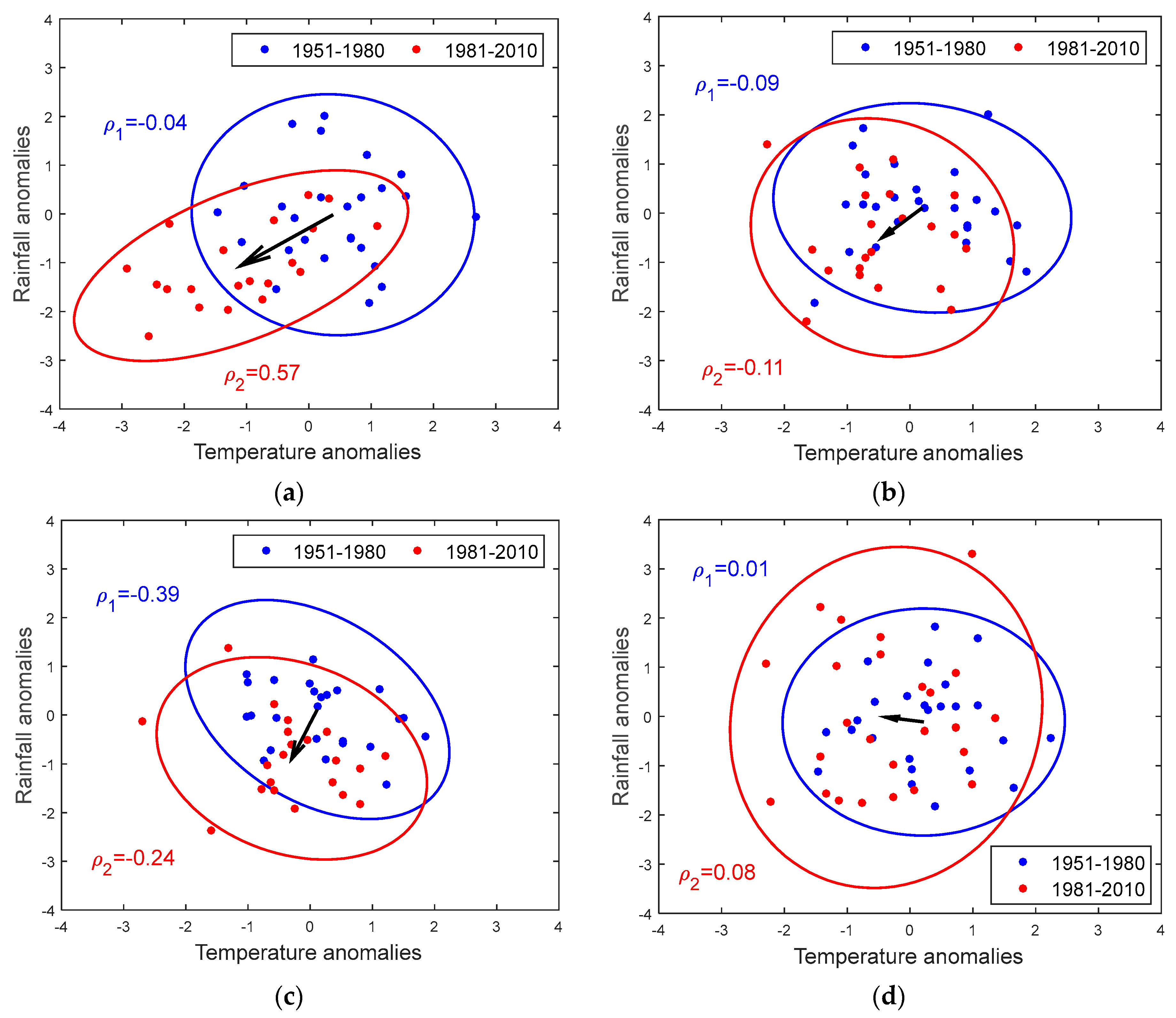
In the winter season, decreasing values of the means for both the seasonal temperature and rainfall anomalies have been detected passing from 1951–1980 to 1981–2010 in all the selected gauges, except for a weak increase of the seasonal rainfall of gauge 1680 (Table 4). These results are clearly evidenced by the translations of the centroids of the ellipses (Figure 2a–d). The t-test, adopted for the verification of these changes in a separate way for and , provides statistically significant results in six out of eight cases (Table 5). Specifically, the rigid translation of the ellipses proved to be significant for both the winter temperature and rainfall of gauges 930 (with remarkable values of −1.5 and −1.0, respectively) and 1010, while in the other two gauges, this is only verified by one variable ( of gauge 1180 and of gauge 1680), as shown in Table 4. The statistical significance of the change in the means’ vector, jointly assessed by means of the multivariate Hotelling’s test, was provided for all the cases, confirming the results obtained though the t-test (Table 5). The rotation assumes a high significant value for gauge 930 (109.1°). The deformations are always not significant, with the highest not-significant increase of 61% observed in gauge 1680 (Table 4).
In spring, Figure 3a,b shows that both the stations which satisfy the normality hypothesis present decreasing tendencies of temperature and rainfall anomalies, but only gauge 930 (Figure 3a) evidences a significant clear negative tendency (−0.8) of the temperature anomalies (Table 4). The Hotelling’s test is verified in spring only for gauge 930, and the t-test is verified for the same gauge only for the temperature anomalies. For the rotations, the only significant value has been observed at gauge 930 (69.2°), while not-significant values were detected regarding the deformations.
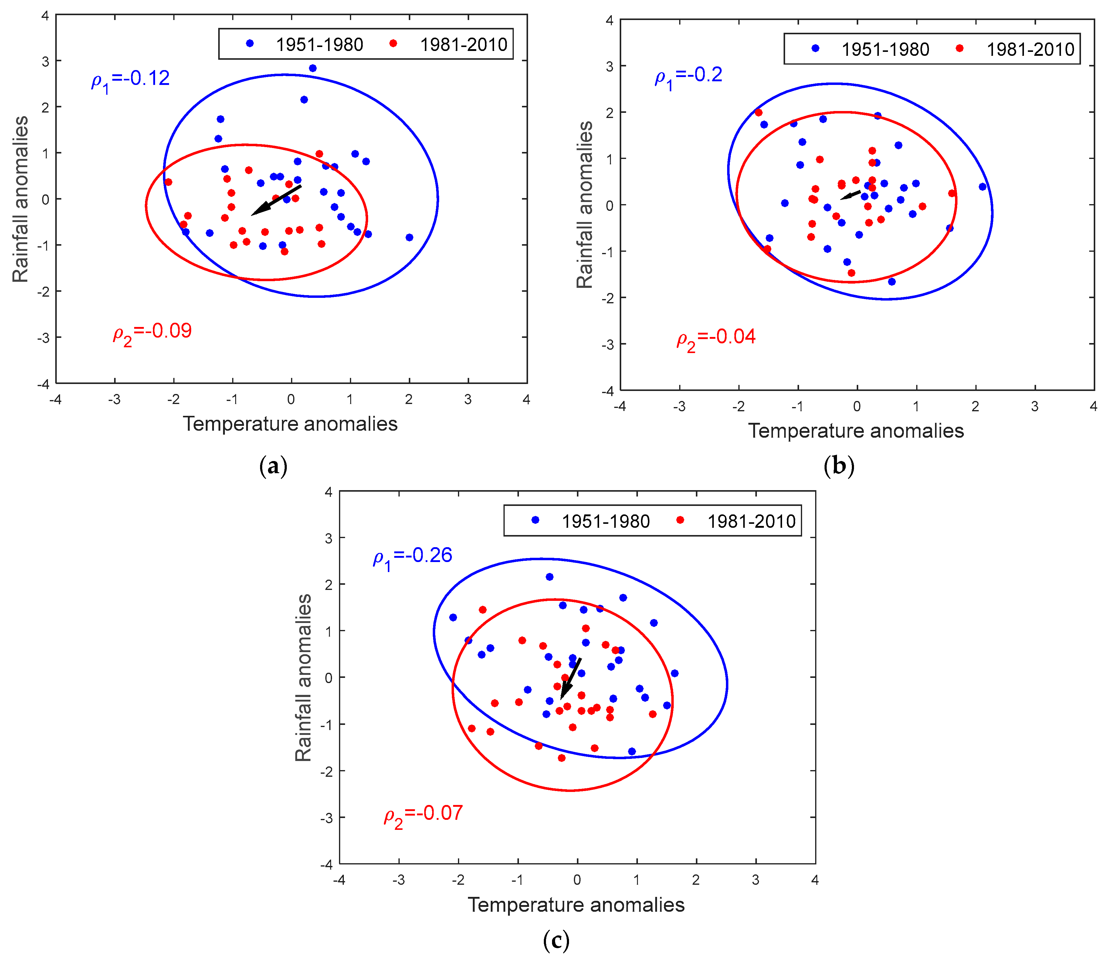
In autumn (Figure 4a–c), notable statistically significant decreasing values (Table 4) have been observed. In particular, gauge 930 (Figure 4a) evidences a more pronounced significant negative tendency for the mean temperature anomalies than for the rainfall ones (−0.8 and −0.6 for the temperature and the rainfall anomalies, respectively), as detected through the t-test. Gauge 1180 presents the only significant value only for the rainfall anomalies (−0.8). These results have been statistically proved also by means of the multivariate Hotelling’s test (Table 5). Not-significant values were observed for the rotations, and the only significant value of deformation has been detected at gauge 930 (−59%).
4. Conclusions
The variabilities of the seasonal temperature and rainfall observed in four sites located in Calabria (Southern Italy) have been jointly investigated by means of the analysis of the variations in the 95% confidence ellipses of the bivariate normal distribution, evaluated for two different 30-year periods. The values of the various displacements (translations, rotations, and deformations) detected for the ellipses, estimated passing from the first subperiod to the second one, have been presented. Though this study is limited to a few gauges, the joint variations of the two climatic variables show the same tendencies in most of the considered cases. The results confirm the general negative trend detected for both monthly temperature and rainfall in Southern Italy, detected in previous studies [14,33]. Moreover, the tendency detected for seasonal rainfall confirms the general trend of long-term cumulated precipitation in the Mediterranean area [6,24]. On the contrary, the results here obtained for temperature evidenced that global warming, also revealed in the Mediterranean and the Middle East [24], is not always observed everywhere and in each season of the year, because opposite trends linked to specific local features can be detected, as already evidenced in Calabria by Caloiero et al. [23]. Moreover, it is important to highlight that when the comparison is carried out on results based on datasets with substantial differences, only limited conclusions about trends can be drawn. Nevertheless, even if the obtained results in terms of the joint gradients of rainfall and temperature statistics cannot be used to predict their relationships, because no assessment about the stationarity of the results was carried out, the trends observed, if confirmed in the future, could have potential impacts on several environmental sectors, in particular on agriculture.
Author Contributions
Conceptualization, E.F., R.C. and B.S.; Methodology, Software and Validation, E.F., R.C. and B.S.; Formal Analysis and Investigation, E.F. and R.C.; Writing-Review & Editing, E.F. and R.C.
Conflicts of Interest
The authors declare no conflict of interest.
References
- Calderini, D.F.; Abeledo, L.G.; Savin, R.; Slafer, G.A. Effect of temperature and carpel size during pre-anthesis on potential grain weight in wheat. J. Agric. Sci. 1999, 132, 453–459. [Google Scholar] [CrossRef]
- Abbate, P.E.; Dardanelli, J.L.; Cantarero, M.G.; Maturano, M.; Melchiori, R.J.M.; Suero, E.E. Climatic and water availability effects on water-use efficiency in wheat. Crop Sci. 2004, 44, 474–483. [Google Scholar] [CrossRef]
- Medori, M.; Michelini, L.; Nogues, I.; Loreto, F.; Calfapietra, C. The impact of root temperature on photosynthesis and isoprene emission in three different plant species. Sci. World J. 2012. [Google Scholar] [CrossRef] [PubMed]
- Caloiero, T. Analysis of rainfall trend in New Zealand. Environ. Earth Sci. 2015, 73, 6297–6310. [Google Scholar] [CrossRef]
- Brunetti, M.; Caloiero, T.; Coscarelli, R.; Gullà, G.; Nanni, T.; Simolo, C. Precipitation variability and change in the Calabria region (Italy) from a high resolution daily dataset. Int. J. Climatol. 2012, 32, 57–73. [Google Scholar] [CrossRef]
- Longobardi, A.; Buttafuoco, G.; Caloiero, T.; Coscarelli, R. Spatial and temporal distribution of precipitation in a Mediterranean area (Southern Italy). Environ. Earth Sci. 2016, 75, 189. [Google Scholar] [CrossRef]
- Mehta, A.V.; Yang, S. Precipitation climatology over Mediterranean Basin from ten years of TRMM measurements. Adv. Geosci. 2008, 17, 87–91. [Google Scholar] [CrossRef]
- Reale, M.; Lionello, P. Synoptic climatology of winter intense precipitation events along the Mediterranean coasts. Nat. Hazards Earth Syst. 2013, 13, 1707–1722. [Google Scholar] [CrossRef]
- Lionello, P.; Giorgi, F. Winter precipitation and cyclones in the Mediterranean region: Future climate scenarios in a regional simulation. Adv. Geosci. 2007, 12, 153–158. [Google Scholar] [CrossRef]
- Brunetti, M.; Maugeri, M.; Monti, F.; Nanni, T. Temperature and precipitation variability in Italy in the last two centuries from homogenised instrumental time series. Int. J. Climatol. 2006, 26, 345–381. [Google Scholar] [CrossRef]
- Longobardi, A.; Villani, P. Trend analysis of annual and seasonal rainfall time series in the Mediterranean area. Int. J. Climatol. 2010, 30, 1538–1546. [Google Scholar] [CrossRef]
- Piccarreta, M.; Capolongo, D.; Boenzi, F. Trend analysis of precipitation and drought in Basilicata from 1923 to 2000 within a Southern Italy context. Int. J. Climatol. 2004, 24, 907–922. [Google Scholar] [CrossRef]
- Liuzzo, L.; Bono, E.; Sammartano, V.; Freni, G. Analysis of spatial and temporal rainfall trends in Sicily during the 1921–2012 period. Theor. Appl. Climatol. 2016, 126, 113–129. [Google Scholar] [CrossRef]
- Caloiero, T.; Buttafuoco, G.; Coscarelli, R.; Ferrari, E. Spatial and temporal characterization of climate at regional scale using homogeneous monthly precipitation and air temperature data: An application in Calabria (southern Italy). Hydrol. Res. 2015, 46, 629–646. [Google Scholar] [CrossRef]
- Klok, E.J.; Tank, A. Updated and extended European dataset of daily climate observations. Int. J. Climatol. 2009, 29, 1182–1191. [Google Scholar] [CrossRef]
- Caloiero, T.; Callegari, G.; Cantasano, N.; Coletta, V.; Pellicone, G.; Veltri, A. Bioclimatic Analysis in a Region of Southern Italy (Calabria). Plant Biosyst. 2015. [Google Scholar] [CrossRef]
- Liang, K.; Bai, P.; Li, J.J.; Liu, C.M. Variability of temperature extremes in the Yellow River basin during 1961–2011. Quat. Int. 2014, 336, 52–64. [Google Scholar] [CrossRef]
- Caloiero, T. Trend of monthly temperature and daily extreme temperature during 1951–2012 in New Zealand. Theor. Appl. Climatol. 2016. [Google Scholar] [CrossRef]
- Salinger, M.J.; Griffiths, G.M. Trends in New Zealand daily temperature and rainfall extremes. Int. J. Climatol. 2001, 21, 1437–1452. [Google Scholar] [CrossRef]
- Donat, M.G.; Alexander, L.V. The shifting probability distribution of global daytime and night-time temperatures. Geophys. Res. Lett. 2012, 39, L14707. [Google Scholar] [CrossRef]
- Giorgi, F. Climate change hot-spots. Geophys. Res. Lett. 2006, 33, L08707. [Google Scholar] [CrossRef]
- Simolo, C.; Brunetti, M.; Maugeri, M.; Nanni, T.; Speranza, A. Understanding climate change–induced variations in daily temperature distributions over Italy. J. Geophys. Res. 2010, 115, D22110. [Google Scholar] [CrossRef]
- Caloiero, T.; Coscarelli, R.; Ferrari, E.; Sirangelo, B. Trend analysis of monthly mean values and extreme indices of daily temperature in a region of southern Italy. Int. J. Climatol. 2017, 37, 284–297. [Google Scholar] [CrossRef]
- Tanarhte, M.; Hadjinicolaou, P.; Lelieveld, J. Intercomparison of temperature and precipitation data sets based on observations in the Mediterranean and the Middle East. J. Geophys. Res. 2012, 117. [Google Scholar] [CrossRef]
- Rajeevan, M.; Pai, D.S.; Thapliyal, V. Spatial and temporal relationships between global land surface air temperature anomalies and Indian summer monsoon rainfall. Meteorol. Atmos. Phys. 1998, 66, 157–171. [Google Scholar] [CrossRef]
- Huang, Y.; Cai, J.; Yin, H.; Cai, M. Correlation of precipitation to temperature variation in the Huanghe River (Yellow River) basin during 1957–2006. J. Hydrol. 2009, 372, 1–8. [Google Scholar] [CrossRef]
- Cong, R.G.; Brady, M. The Interdependence between Rainfall and Temperature: Copula Analyses. Sci. World J. 2012. [Google Scholar] [CrossRef] [PubMed]
- Péguy, C.P. Une tentative de délimitation et de schématisation des climats intertropicaux. Rev. Geogr. 1961, 36, 1–6. [Google Scholar] [CrossRef]
- Craddock, J.M. Methods of comparing annual rainfall records for climatic purposes. Weather 1979, 34, 332–346. [Google Scholar] [CrossRef]
- Wilks, D.S. Statistical Methods in the Atmospheric Sciences, 2nd ed.; International Geophysics Series; Academic Press: Cambridge, MA, USA, 1995. [Google Scholar]
- Rodrigo, F.S. On the covariability of seasonal temperature and precipitation in Spain, 1956–2005. Int. J. Climatol. 2014, 35, 3362–3370. [Google Scholar] [CrossRef]
- Sirangelo, B.; Ferrari, E. Probabilistic analysis of the variation of water resources availability due to rainfall change in the Crati basin (Italy). In Global Change: Facing Risks and Threats to Water Resources; Servat, E., Demuth, S., Dezetter, A., Daniell, T., Ferrari, E., Ijjaali, M., Jabrane, R., van Lanen, H., Huang, Y., Eds.; IAHS Publication, N° 340; IAHS Press: Wallingford, UK, 2010; pp. 142–149. [Google Scholar]
- Ferrari, E.; Terranova, O. Non-parametric detection of trends and change point years in monthly and annual rainfalls. In Proceedings of the 1st Italian-Russian Workshop on New Trend in Hydrology, CNR-IRPI, Rende, Italy, 24–26 September 2002; pp. 177–188. [Google Scholar]
- Kottegoda, N.T.; Rosso, R. Applied Statistics for Civil and Environmental Engineers, 2nd ed.; Wiley & Sons: New York, NY, USA, 2008. [Google Scholar]
- Hotelling, H. The generalization of Student’s ratio. Ann. Math. Stat. 1931, 2, 360–378. [Google Scholar] [CrossRef]
Figure 1.
Location of the selected gauges in the Calabria region.

Figure 2.
The 95% confidence ellipses for the winter season at gauge (a) 930; (b) 1010; (c) 1180; (d) 1680.
Figure 2.
The 95% confidence ellipses for the winter season at gauge (a) 930; (b) 1010; (c) 1180; (d) 1680.

Figure 3.
The 95% confidence ellipses for the spring season at gauge (a) 930; (b) 1010.
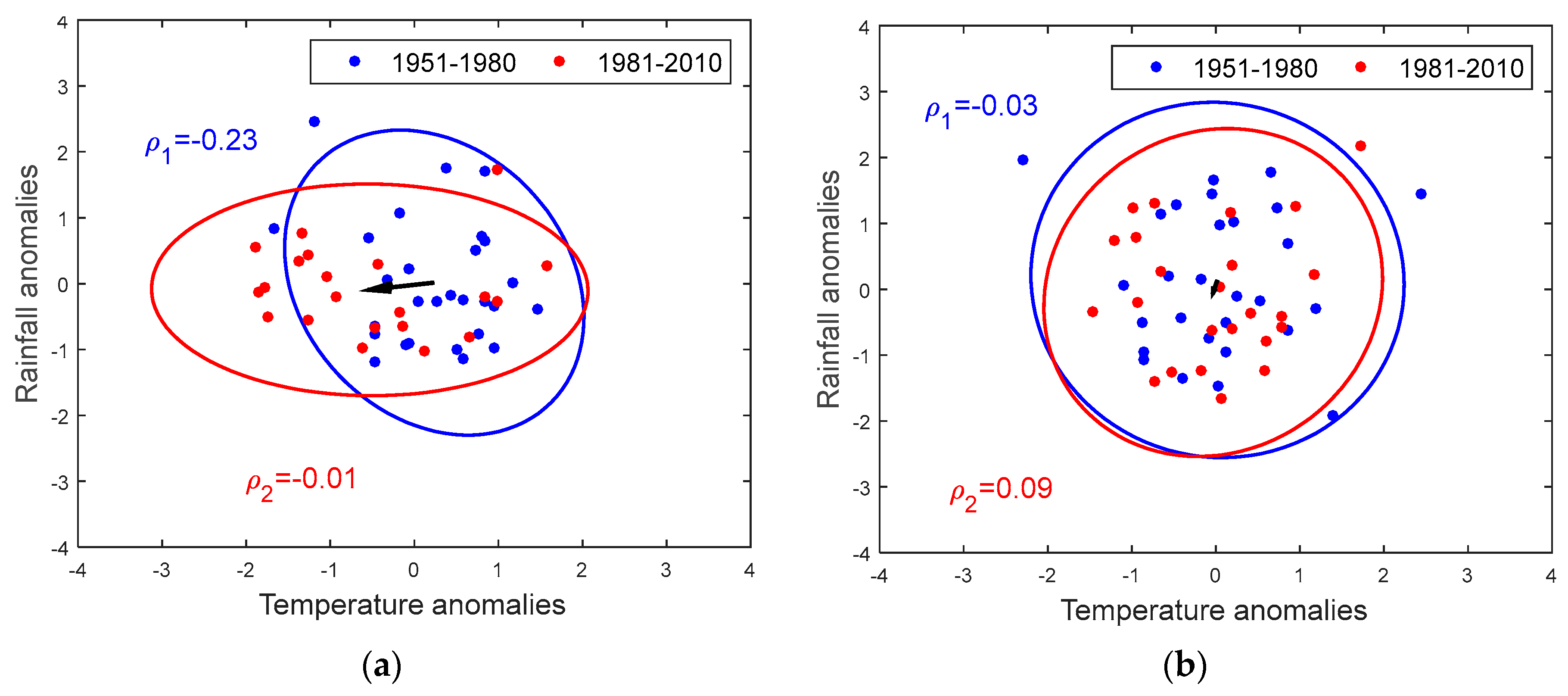
Figure 4.
The 95% confidence ellipses for the autumn season at gauge (a) 930; (b) 1010; (c) 1180.


Table 1.
Percentages of missing values of monthly mean temperature and cumulated rainfall.
| Missing Data (%) | |||||||
|---|---|---|---|---|---|---|---|
| Monthly Temperature | Monthly Rainfall | ||||||
| Code | Station | 1951–1980 | 1981–2010 | Whole Period | 1951–1980 | 1981–2010 | Whole Period |
| 930 | Villapiana Scalo | 0 | 0 | 0 | 5.8 | 13.6 | 9.7 |
| 1010 | Cosenza | 0 | 0.3 | 0.1 | 7.5 | 9.7 | 8.5 |
| 1180 | Castrovillari | 0 | 4.7 | 2.4 | 5.3 | 9.4 | 7.4 |
| 1680 | Crotone | 3.1 | 5.3 | 4.2 | 8.9 | 11.1 | 10.0 |
Table 2.
Main statistics of temperature and rainfall for the reference period 1961–1990. ( mean daily temperature, : standard deviation of temperature, cumulated rainfall, standard deviation of rainfall).
Table 2.
Main statistics of temperature and rainfall for the reference period 1961–1990. ( mean daily temperature, : standard deviation of temperature, cumulated rainfall, standard deviation of rainfall).
| Season | Station | (°C) | (°C) | ||
|---|---|---|---|---|---|
| Winter | 930 | 10.3 | 0.8 | 231.9 | 81.3 |
| 1010 | 8.6 | 1.1 | 405.4 | 149.0 | |
| 1180 | 9.2 | 1.2 | 371.6 | 134.7 | |
| 1680 | 11.3 | 0.8 | 234.9 | 89.8 | |
| Spring | 930 | 14.9 | 0.9 | 125.2 | 69.0 |
| 1010 | 14.1 | 1.4 | 210.1 | 74.3 | |
| 1180 | 14.6 | 1.2 | 178.0 | 71.2 | |
| 1680 | 15.4 | 1.4 | 117.1 | 60.3 | |
| Summer | 930 | 24.6 | 1.2 | 41.4 | 26.5 |
| 1010 | 24.0 | 1.1 | 64.4 | 36.4 | |
| 1180 | 24.8 | 1.3 | 78.2 | 57.3 | |
| 1680 | 25.3 | 1.1 | 31.9 | 27.7 | |
| Autumn | 930 | 18.5 | 0.9 | 203.5 | 115.1 |
| 1010 | 17.2 | 1.2 | 260.0 | 99.4 | |
| 1180 | 17.8 | 1.1 | 250.1 | 92.1 | |
| 1680 | 19.4 | 0.8 | 250.2 | 117.1 |
Table 3.
Anderson–Darling statistic for temperature and rainfall series. Critical values for different N have been assumed at the 95% confidence level. (The cases in which the normality hypothesis is rejected are in bold italics.)
Table 3.
Anderson–Darling statistic for temperature and rainfall series. Critical values for different N have been assumed at the 95% confidence level. (The cases in which the normality hypothesis is rejected are in bold italics.)
| Season | Gauges | 1951–1980 | 1981–2010 | ||
|---|---|---|---|---|---|
| Temperature | Rainfall | Temperature | Rainfall | ||
| Winter | 930 | 0.229 | 0.249 | 0.189 | 0.473 |
| 1010 | 0.474 | 0.325 | 0.425 | 0.196 | |
| 1180 | 0.472 | 0.707 | 0.392 | 0.224 | |
| 1680 | 0.249 | 0.279 | 0.279 | 0.443 | |
| Spring | 930 | 0.673 | 0.490 | 0.490 | 0.309 |
| 1010 | 0.349 | 0.477 | 0.257 | 0.321 | |
| 1180 | 0.303 | 0.305 | 0.387 | 0.807 | |
| 1680 | 0.790 | 0.899 | 0.261 | 0.218 | |
| Summer | 930 | 0.216 | 0.406 | 1.047 | 0.791 |
| 1010 | 0.264 | 0.351 | 0.309 | 1.154 | |
| 1180 | 0.321 | 1.229 | 0.576 | 0.448 | |
| 1680 | 0.428 | 2.053 | 1.027 | 1.240 | |
| Autumn | 930 | 0.344 | 0.491 | 0.338 | 0.434 |
| 1010 | 0.242 | 0.276 | 0.442 | 0.223 | |
| 1180 | 0.351 | 0.196 | 0.405 | 0.695 | |
| 1680 | 0.346 | 1.015 | 0.190 | 0.863 | |
Table 4.
Displacements of the 95% contour ellipses corresponding to each station and variable passing from 1951–1980 to 1981–2010. (Statistically significant results at 95% confidence level are in bold italics.)
Table 4.
Displacements of the 95% contour ellipses corresponding to each station and variable passing from 1951–1980 to 1981–2010. (Statistically significant results at 95% confidence level are in bold italics.)
| Season | Site | Translations | Rotations | Deformations | |
|---|---|---|---|---|---|
| ϑ (°) | |||||
| Winter | 930 | −1.5 | −1.0 | 109.1 | −16 |
| 1010 | −0.6 | −0.6 | −51.4 | 0 | |
| 1180 | −0.4 | −1.0 | 9.5 | 1 | |
| 1680 | −0.6 | +0.1 | 1.8 | 61 | |
| Spring | 930 | −0.8 | −0.1 | 69.2 | 4 |
| 1010 | −0.1 | −0.2 | −14.9 | −17 | |
| Autumn | 930 | −0.8 | −0.6 | 43.5 | −59 |
| 1010 | −0.2 | −0.1 | 13.5 | −36 | |
| 1180 | −0.3 | −0.8 | −42.8 | −27 | |
Table 5.
Testing results of the change in the means of the seasonal values of temperature (T) and rainfall (R) observed in 1951–1980 and 1981–2010. (H, Hotelling’s test; t(T) and t(R), two-sample t-test. Statistically significant results at the 95% confidence level are in bold italics.)
Table 5.
Testing results of the change in the means of the seasonal values of temperature (T) and rainfall (R) observed in 1951–1980 and 1981–2010. (H, Hotelling’s test; t(T) and t(R), two-sample t-test. Statistically significant results at the 95% confidence level are in bold italics.)
| Season | Site | H | t(T) | t(R) |
|---|---|---|---|---|
| Winter | 930 | 30.28 | −4.84 | −3.91 |
| 1010 | 11.66 | −2.39 | −2.19 | |
| 1180 | 23.77 | −1.59 | −3.88 | |
| 1680 | 4.91 | −2.18 | +0.28 | |
| Spring | 930 | 8.70 | −2.85 | −0.48 |
| 1010 | 0.46 | −0.21 | −0.65 | |
| Autumn | 930 | 17.39 | −3.05 | −2.51 |
| 1010 | 1.37 | −0.98 | −0.51 | |
| 1180 | 14.78 | −1.24 | −3.36 |
© 2018 by the authors. Licensee MDPI, Basel, Switzerland. This article is an open access article distributed under the terms and conditions of the Creative Commons Attribution (CC BY) license (http://creativecommons.org/licenses/by/4.0/).
Share and Cite
MDPI and ACS Style
Ferrari, E.; Coscarelli, R.; Sirangelo, B. Correlation Analysis of Seasonal Temperature and Precipitation in a Region of Southern Italy. Geosciences 2018, 8, 160. https://doi.org/10.3390/geosciences8050160
AMA Style
Ferrari E, Coscarelli R, Sirangelo B. Correlation Analysis of Seasonal Temperature and Precipitation in a Region of Southern Italy. Geosciences. 2018; 8(5):160. https://doi.org/10.3390/geosciences8050160
Chicago/Turabian StyleFerrari, Ennio, Roberto Coscarelli, and Beniamino Sirangelo. 2018. "Correlation Analysis of Seasonal Temperature and Precipitation in a Region of Southern Italy" Geosciences 8, no. 5: 160. https://doi.org/10.3390/geosciences8050160
Note that from the first issue of 2016, this journal uses article numbers instead of page numbers. See further details here.