Downscaling Africa’s Drought Forecasts through Integration of Indigenous and Scientific Drought Forecasts Using Fuzzy Cognitive Maps


1
Unit for Research on Informatics for Droughts (URIDA), Central University of Technology, Free State, Private Bag X20539, Bloemfontein 9300, South Africa
2
National Drought Mitigation Center, School of Natural Resources (SNR), University of Nebraska-Lincoln, 815 Hardin Hall, 3310 Holdrege St., Lincoln, NE 68583, USA
*
Author to whom correspondence should be addressed.
Geosciences 2018, 8(4), 135; https://doi.org/10.3390/geosciences8040135
Submission received: 25 November 2017
/
Revised: 25 March 2018
/
Accepted: 9 April 2018
/
Published: 16 April 2018
(This article belongs to the Special Issue Drought Monitoring and Prediction)
Abstract
:In the wake of increased drought occurrences being witnessed in Sub-Saharan Africa, more localized and contextualized drought mitigation strategies are on the agendas of many researchers and policy makers in the region. The integration of indigenous knowledge on droughts with seasonal climate forecasts is one such strategy. The main challenge facing this integration, however, is the formal representation of highly-structured and holistic indigenous knowledge. In this paper, we demonstrate how the use of fuzzy cognitive mapping can address this challenge. Indigenous knowledge on droughts from five communities was modeled and represented using fuzzy cognitive maps. Maps from one of these case communities were then used in the implementation of the integration framework, called ĩtiki.
1. Introduction
Africa continues to be the highest hit by global droughts as well as having the most deaths resulting from these droughts. For instance, 118 out of the 235 world’s droughts that were reported between 2006 and 2015 occurred in Africa. What is more striking is the fact that the 118 droughts (50% of the all droughts) in Africa led to over 99% (20,078 out of 20,251) of the total deaths resulting from the world’s droughts occurring in the same period (2006–2015). Put differently, while 173 people died from the 50% of droughts that occurred in the rest of the world, 20,078 people died from the other 50% of droughts that were recorded in Africa.
Droughts are natural disasters and therefore, cannot be prevented, but they can be mitigated through drought early warning systems (DEWS). DEWS, in turn, require provision and access to timely and reliable climate information [1]. When it comes to Sub-Saharan Africa, there is a complex link between droughts and economic development (or lack of it). In most of these countries, rain-fed agriculture (extremely responsive to climate variability) accounts for over 70% of food production [2]. When droughts strike, governments are forced to redirect budgets initially allocated for developmental projects towards supporting the hungry [3]. For this reason, there are many research, as well as implementation, initiatives geared towards addressing this vicious cycle of droughts facing the region.
Though well-developed drought indices, such as the standard precipitation index (SPI), the Palmer Drought Severity Index (PDSI) and the Effective Drought Index (EDI), perform very well in mapping droughts in spatial and time-scale dimensions, they only detect events that are already happening [4]. El Nino–Southern Oscillation (ENSO) and North Atlantic Oscillation (NAO) are the most developed and most commonly used medium-term drought forecasting indices [5]. One of the drawbacks of these two indices, however, is the fact that they do not forecast the severity of the predicted drought [4]. The use of artificial neural networks (ANNs) to forecast future values of EDI attempts to address this drawback as well as introducing a new addition—forecasting daily drought indices [6].
Seasonal climate forecasts (SCFs) are the main source of drought prediction information in Sub-Saharan Africa. However, despite improvements in the SCFs’ technology and skill, their utilization is still dismal [6,7,8]. Literature-backed evidence indicates that small-scale farmers in Sub-Saharan Africa are still using their indigenous knowledge (IK) on weather to make critical cropping decisions [9,10]. IK is a body of informal folklore [11], associated with the prediction of the weather, which is based on localized knowledge and human observations of the environment. As such, it tends to be more holistic, and more localized to a farmer’s context [12]. Further, this knowledge system has limitations—firstly, it does not offer forecasts beyond a season [13], and secondly, meteorologists continue to treat this knowledge as superstition, partly because there are no means of scientifically evaluating and validating it.
IK systems are dynamic and change after human innovation and interaction with other knowledge systems [12,13,14]. Conversely, modern weather forecasting is a scientific process that estimates weather prospects based on concepts such as hotness and rainfall [15]. Some modern methods predict daily weather based on fuzzy concepts and testing of meteorological premises [16]. Researchers have advocated for SCFs as a measure to represent the impact of droughts [17]. In this regard, SCFs could help to prepare for, and adapt to, droughts.
There is consensus that, in the face of droughts, solutions that focus on local actors and ‘at risk’ communities are key to humanitarian responses’ effectiveness. To this end, there have been renewed efforts towards promoting IK and how to integrate it with SCFs [10,18,19,20,21] The main hindrance to this integration is the representation of IK in ways that can allow its integration with SCFs. In this paper, we present a formal method for analyzing and representing IK. We achieve this by way of leveraging the ability of fuzzy cognitive maps to model imprecise data and nonlinear functions of arbitrary complexity.
Indigenous knowledge and modern, science-based weather forecasting approaches are not mutually exclusive, but significant discordance between the two is still apparent. Clear understanding and careful integration of IK presents opportunities, especially in the dissemination process of drought forecasts, to farmers in Sub-Saharan Africa (SSA). IK supports ways that are culturally appropriate and locally relevant. There is a common departure whereby generally (not just in climate and weather information), integrating indigenous knowledge into modern science can improve livelihoods [22,23,24,25,26]. Integrated approaches aimed at giving communities several levels of risk-preparedness are desirable.
Over the last decade, initiatives towards integrating these two systems have increased two-fold, especially in the area of environmental conservation [27,28,29,30]. Though this integration has potential to bring several benefits, the diverse nature of the two makes it a daunting task [31]. For instance, IK is highly informal and tacit—it is often represented using vague linguistic variables [32]. On the contrary, its scientific counterpart is explicit and highly structured [31]. If IK is to be integrated with scientific knowledge and eventually be used in decision-making processes, there is a need to represent IK in an explicit, structured way; fuzzy cognitive maps are one way of achieving this. This is because other approaches that employ subjective and qualitative approaches may not capture the holistic nature of IK whose concepts are not precise.
Fuzzy logic was conceptualized by [33] and is defined as a convenient way to map an input space to an output space. Fuzzy cognitive mapping (FCM) is a combination of fuzzy logic and cognitive mapping; it is a way to represent knowledge in systems that are characterized by uncertainty and complex processes [34]. FCM has proven efficient for solving problems in which a number of decisions and uncontrollable variables are causally interrelated [35]. FCMs can be used to exploit causal knowledge and experience which has been accumulated over a certain period of time on a complex phenomenon [36,37,38,39]. FCM is developed using human knowledge experts who know the operation of a particular system and its behaviour under different circumstances [40].
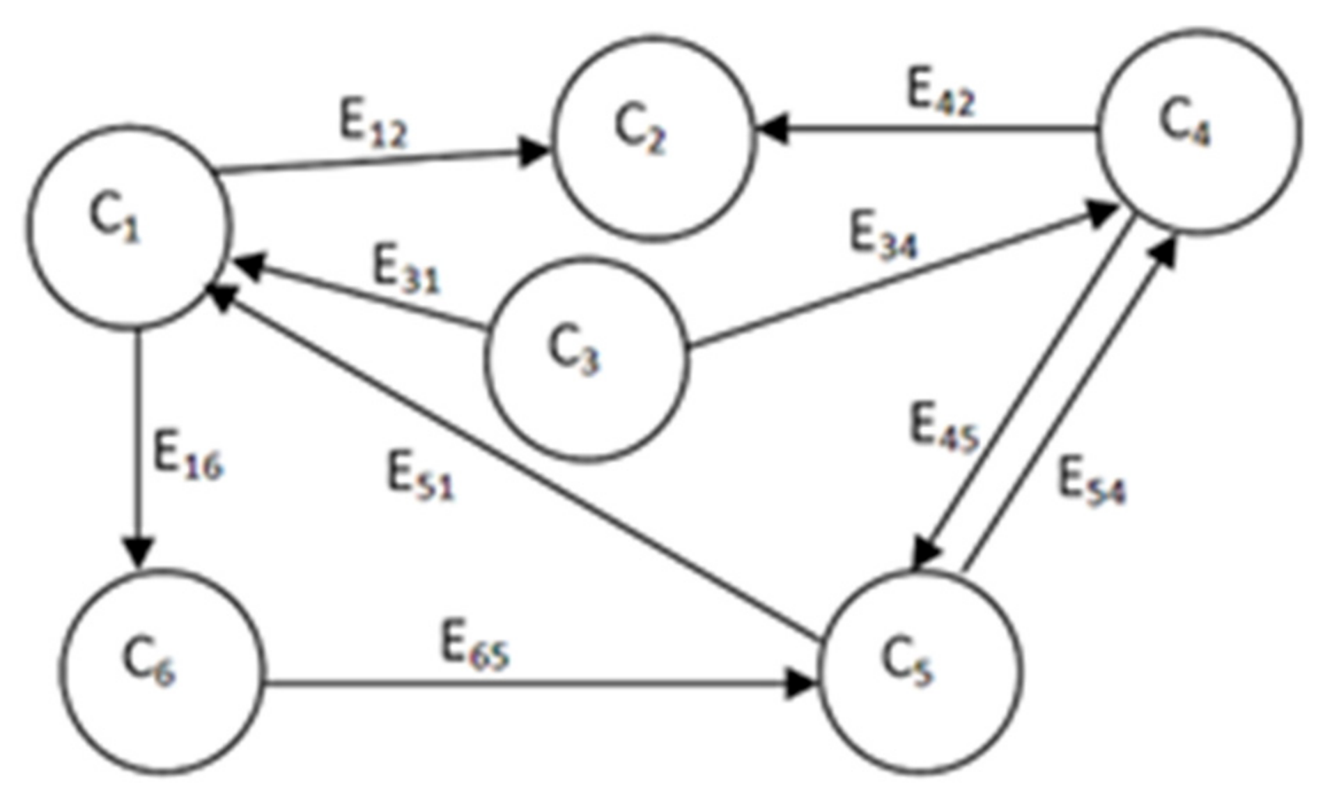
FCMs work efficiently with missing data to model systems with nonlinearities and surrounding uncertainty [41]. FCMs use artificial neural network techniques that incorporate ideas from fuzzy logic to create decision support systems [40,41,42,43] To come up with a universal FCM, knowledge from different experts can be accumulated through combining several FCMs into one FCM by merging same concepts [35,44,45]. A FCM is represented as a directed graph (Figure 1) in which each node represents a concept(the edge, Eij, from causal concept Ci to concept Cj measures how much Ci causes Cj, with Eij taking values in a fuzzy causal interval [0, 1] or [−1, 1] based on system specifics [46]).
- Eij = 0 indicates no causality;
- Eij > 0 indicates causal increase, i.e., Cj increases as Ci increases;
- Eij < 0 indicates causal decrease or negative causality i.e., Cj decreases as Ci increases.
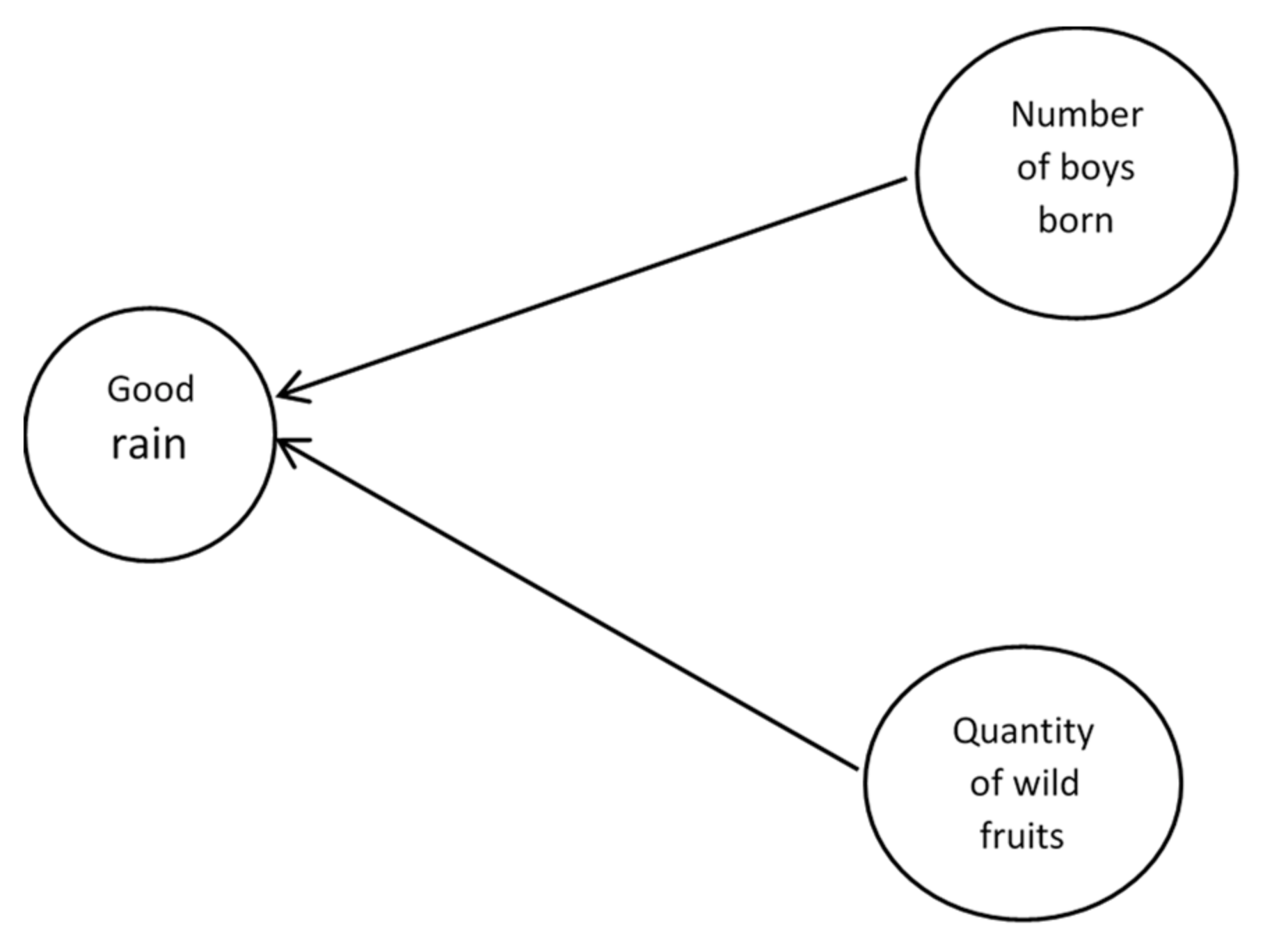
As an example, an FCM based on IK can be used to depict that the number of human boys born and the quantity of wild fruits influences the quality of rains (as shown in Figure 2).
The direction of the arrows represents causal relationships between two concepts, while the weights characterize the strength of the causal relationships [44,45]. For instance, a directed edge Wij, representing the weight between concept Ci and concept Cj, is a measure of how much Ci causes Cj [47]. Therefore, in FCM, the state of a node, Ci, is determined by the sum of its inputs modified by causal link weights [35,44] and a nonlinear transfer function, S, as shown in Equation (1) [42].
FCM models can be tested dynamically through simulations where scenarios are introduced and predictions made by indigenous knowledge viewing dynamically the consequences of the corresponding actions [38,43,44,47]. To get complex personal knowledge concerning concepts, controlled interviews can be used and information transcription from recorded interviews to the concept maps formalized. FCMs are recorded in the form of matrices of relationships between concepts [44,48,49].
Learning methods can be employed with multiple concepts to improve the speed of the learning process and the quality of learning FCMs to construct a causal graph based on historical data. Prediction algorithms can also be constructed in FCM using the fuzzy c-means clustering algorithm, in which a genetic algorithm is applied to learn weights of the FCM. Using this method, a fully learned FCM can be used to symbolize preserved fuzzy logic relationships of fuzzy time series and form predictions. Further, FCMs can be designed using crisp decision trees (an intelligent technique that extracts rules from both symbolic and numeric data) that have been fuzzified [35,45,50]. Fuzzy rules can be combined and used to express non-monotonic causality in FCMs along with aggregation operators to combine multiple causal influences. In situations where domain experts are not able to express causal relationships, data driven methods can be used to learn FCMs.
2. Materials and Methods
2.1. Data Sources
Data sources considered in this research were both primary—acquired using interviews and case studies—as well as secondary data from a literature review. The aim of this investigation was to identify the main characteristics of indigenous knowledge that are used in drought forecasting within the identified communities.
2.1.1. Source 1: Indigenous Knowledge on Drought Forecast Indicators from the Literature
Four case studies were reviewed. The objective of this review was to identify common features and classifications of IK in drought forecasting. Below is the description of each of these four case studies:
Monze and Sinazonmgwe, Zambia
Here, a good season is characterized by the presence of certain types of birds/insects, mist in hills during the dry season as well as by plenty of wild fruits. Other indicators for a good season are an abundance of leaves on fig trees, more (than male) female births among humans, high temperatures, frost around the end of the year and dark and heavy clouds. A bad season is characterized by less wild fruits, the failure of mukololo trees to flower, sparse leaves on fig trees, more human male children births, and finally, very cold winters between May and August [9].
Lupane and Lower Gweru, Zimbabwe
A good season is characterized by a heavy production of fruits by Rhus lancea and Lancea discoloring trees and non-fruiting of Azanzagarikeana. Heat waves are also experienced, characterized by a lot of cicadas; early haziness soon after winter is witnessed. Further, north-easterly winds, the prevalence of whirlwinds, frogs turning brownish, rain-birds making a lot of noise and the appearance of butterflies from the north starting in October indicate a good season. A bad season is identified by opposing observations (to those of a good season), such as Rhus lancea and Lancea producing few fruits, discoloration of Lancea which then produces fruit but aborts it before the rain. An extended winter period is also a sign of a bad season. North-easterly winds are also dominant, white frogs appear in trees, lots of thunderstorms occur without rain and rain starts from early October [9].
Rakai District, Uganda
Indicators that rain will fall in a week’s time include an increase in night time temperature, a shift in the direction of prevailing winds from easterlies to westerlies or a shift from southerlies to northerlies and flowering of trees, especially coffee trees. Others are particular phases of the moon (rain is more likely during the dark phase of the moon), the appearance of whirlwinds that lift dust and leaves as well as arrival of migratory birds, particularly the Abyssinian hornbill (Bucorvusabyssinicus). This bird’s call is said to resemble the Luganda word, ggulu, which means “heaven”, and to connote the phrase, ggulumpaenkuba or “heaven, send rain”. [51].
Wajir in Kenya
Somalis live in the Northeastern part of Kenya, and their main economic activity is pastoralism. For Somalis, the most trusted indicators are to do with their domestic animals with which they spend most of their lives. The Somalis occupy a semi-arid region, Wajir, which lies within the Sahelian climatic region. The region is characterized by long dry spells and short rainy seasons (annual average rainfall is between 250 mm and 300 mm). Most of the areas in Wajir, therefore, are 100% arid. Due to continentality and low altitude, Wajir experiences high temperatures with an annual mean of 28 °C. Droughts are very rampant in Wajir and when they occur, they lead to a very large number of deaths of livestock, which leaves the community very vulnerable [52]. With an area of 56,501 kilometers squared (about 10% of Kenya’s land mass), Wajir is home to an approximated population of 521,000. Over 70% of this population practice nomadic pastoralism, with camels and cattle being the most dominant livestock [53,54].
Indicators from the Somali community are described below. These indicators are associated with the four main seasons experienced in the area.
January-February-March (Jilaal) are the hottest (over 30 °C) months, characterized by clear clouds and meteorological indicators such as:
- Failure of the out of season showers expected on the 56th day (towards the end of February) is an indicator of a bad season and
- Failure of the out of season showers expected on the 70th day (second week of March) is an indicator of a bad season.
Indicators associated with animal behavior include
- When a drought is looming in the coming season, cattle take on excessive water and refuse, or are reluctant to, move away from the watering point;
- When cattle take water and run around jovially as if in a celebration mood, this predicts a good season (rain) on the way;
- When cows give birth to female calves, the community should prepare for a bad season (drought);
- Cattle bulls become “arrogantly playful” when the coming season is going to be good;
- Female camels urinate while sitting as if to express hopelessness for the future; and
- A sudden increase in libido, mating and general excitement of livestock symbolizes the rain season approaching.
April-May-June (Guu) is wet and represents the long, rainy season. Nimbus clouds cover the sky and the nights are very cold. The indicators for this season include
- If rain starts early in the morning, the community should prepare their cattle and land as it symbolizes good seasonal harvest and plenty of pasture for livestock during that season;
- Failure of mid-season showers expected on the 90th day is an indicator of a bad season
- Failure of peak season showers expected on the 90th day (which is on 15th of April) is an indicator of a bad season and
- One astronomical indicator states that if there is a shooting star on a Tuesday, camels will soon get stuck in mud, and this symbolizes heavy (adequate) rain on the way.
Indicators associated with animal behavior during this season are
- The jovial mood of camels is an indication that the coming season will be good;
- Grunting of camel bulls (making mating calls) symbolizes a good rainy season;
- If the cattle refuse to go back to home and run away while facing different directions, it is a sign of a bad season;
- If cattle run towards their home around 3 o’clock in the afternoon, this shows that a good season (rain) is coming and
- When cattle make specific throat vocal sounds when sleeping at night, this is an indicator that the coming season is going to be good; other vocals represent a bad season.
An indicator associated with birds’ behavior is that when the bird called IrrKujira makes noise between midnight and early in the morning, this is a sign of a season with good rain. Further, an indicator associated with insects’ behavior states that when black ants make and follow only one route from their hole, this is an indicator of a bad season. If the ants make more than four routes from their holes, it shows a good season is looming.
July-August-September (Hagaay) is characterized by dry and cold as well as cool weather and a low evaporation rate that favors the continuous growth of vegetation. Animal behavior indicators include
- When camels run away browsing haphazardly and appear to have lost their hearing senses, this depicts a bad season;
- When camels brush their legs together, this is a good indication of a bumper season and
- When moles throw up soil, making the sand loose for aeration, this depicts a very hot season.
October-November-December (Deyr) is wet and is characterized by short periods of rain, high temperatures and unpredictable clouds. The main indicator here is meteorological in nature. The indicator states that “if the short rains start early in the morning, get prepared with your camel and shoats—seasonal rains are going to be good for browsers (camel and goats), but there will be no grass for cattle”.
Common Features of IK on Drought Forecasting
From the above case studies, it can be seen that the indicators are very specific to a location. Subjective terms, such as ‘good yield’ and ‘bad season’, are only put into context at local levels and for specific seasons. The indicators also reflect the main economic activities that the community indulges in. For instance, the indicators for cattle keepers will be different from those of a crop farmer. The general consensus, however, is that some aspects of IK, such as the behavior of birds/animals, are difficult a model to represent. Approaches for assessing the scientific validity of these indicators have also not been developed. Further, their interpretation is in the context of a given season, for example, July-August-September (Hagaay) in the case of Somalis.
A further finding from the case studies above is that IK in drought forecasting in the tropics falls into six general categories: (1) patterns of seasons (cold, dry, hot, rainy); (2) animal, insects and birds’ behaviors; (3) astronomical; (4) meteorological; (5) human nature and behavior; and (6) the behavior of plants/trees, for example fruit and flower production. Further, it must be noted that in applying indigenous knowledge to predict drought-related events, communities have informal ranking systems based on factors such as the source (who reported the indicator) and coverage (how widespread it is).
2.1.2. Source 2: Primary Data Collection
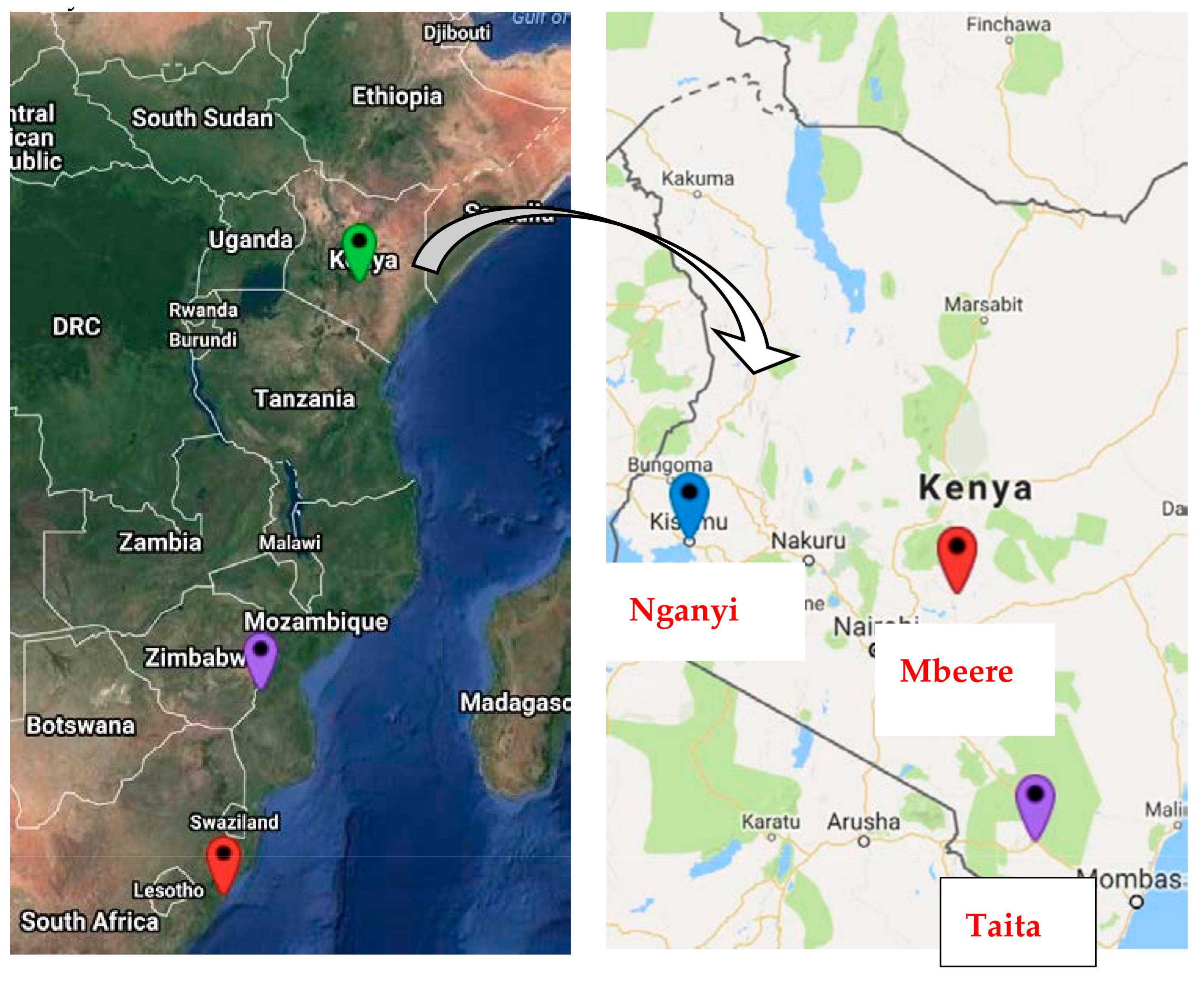
Using a series of structured interviews [55,56] primary data was collected from five communities—see a sample extract of the questionnaire in the Appendix A. Three of these communities live in Kenya, one in South Africa and the fifth one is found in Mozambique. The first data collection was carried out among the Mbeere people in Eastern Kenya, between September and December 2011, while the second case study was carried out among the Nganyi people in Western Kenya between February and March 2012. Subsequently, using the experience from these two case studies, a third set of data was collected (between November and December 2013) from Muchenedze, a place located in the Mossurize district, in Manica Province of Mozambique. The fourth data set (collected between April and May 2014) was from KwaZulu Natal in South Africa, while the fifth case study, carried out between June and July 2014, was from Taita-Taveta in Kenya (Figure 3).
In all five case studies, the people interviewed, with the help of research assistants from the communities, were members of the studied communities. The purposive sampling method [15] was used to select 50 respondents for each case. The research assistants were trained with regard to interpretation of the interviewing guidelines and research ethics. The main objective of using structured interviews was to understand the respondents’ points of view so that individual opinions about indigenous knowledge on drought forecasts could be elicited. In order to place the data into context, other aspects of the interview included respondents’ demographics (age, gender, education level, home village and occupation), levels of seasonal climate forecast awareness, mobile phone ownership/usage and the weather stations’ coverage of the target location.
Qualitative research [55] was then used to describe causal links between indigenous drought indicators and drought outcomes. Quantitative methods were used to establish statistically significant conclusions about the populations in the case study locations by analyzing the collected data from a representative sample of the population. These indicators were recorded by scales of magnitude of effects between the concepts (strong negative, negative, none, positive and strong positive). The collected data was set up in a Statistical Package for Social Sciences (SPSS) codebook. In order to derive common knowledge, the data was analyzed using both quantitative (such as percentage and number of respondents) and descriptive statistics (such as mode and mean of categorical responses). The analyzed data was represented as group knowledge (on visual astronomical and meteorological weather concepts and causal effects on short term weather) using statistical summaries.
Case Study 1: Mbeere, Kenya
With an average of 750 mm (most parts receive less than 550 mm) annual rainfall, Mbeere is classified as an Arid and Semi-Arid Land (ASAL). Between 50% and 85% of the land is arid (Republic of Kenya, 2008). Mbeere’s terrain is characterized by scattered outcropping hills and the extensive altitudinal range of the area influences the temperature, which ranges from 15 °C to 30 °C. The main source (over 80%) of livelihood is rain-fed marginal farming and livestock (agro-pastoralists) keeping. This being the case, the farmers here rely mostly on the knowledge of seasons in making cropping decisions. Like most parts of Kenya, there are two main rainy seasons experienced in Mbeere: the March-April-May (MAM) long rains and the October-November-December (OND) short rains. Crops grown include maize, sorghum, millet, beans, cowpeas, green grams, pigeon peas, cotton and tobacco on farms with an average size of 3.5 Ha. Livestock kept include cattle (Zebu mostly), goats, sheep, poultry, donkeys and bees.
The 50 respondents interviewed were drawn from several villages covering over a third of the region. The respondents were mostly semi-literate small-scale/peasant agro-livestock female farmers over 20 years of age. There were many more literate men than women; the number of illiterate people dropped with a decrease in age. There were generally more men who owned mobile phones than women, however, all (except one) people that did not have a phone, used phones, mostly from relatives. The lack of relevant weather information among the respondents motivated their willingness to receive forecasts by mobile phone—89% of them said that they would like to receive weather information via mobile phone. Like in most other communities/regions, the indigenous weather/drought indicators among the Mbeere people are associated with seasons. The diversity, level of detail and systematic nature of the indicators from the respondents confirmed that the community has very rich IK systems that help the people cope with, and adapt to, the environment—mixed agriculture, for example. A complete list of these indicators was compiled and classified according to five main seasons: January–February, dry season; March-April-Mary, long rains; June–July, cold season; August–September, dry season and October-November-December, short rains. Below are the details of the identified indicators.
(a) January–February
This period forms the transition between the OND and MAM rain seasons. In a normal season, the OND rains end in the second week of December and the MAM starts in the second week of March.
Meteorological
- Moderate temperatures (less than 25 °C) are considered good because this ensures that the annual crops (cotton and pigeon peas) survive until the MAM rains.
Flower, Leaf and Fruit Production:
- Good yields by mango trees that produce large fruits (e.g., ndoto) are a good sign, the opposite indicates a poor season, and
- Good yields from some wild fruits such as ngaa are a bad sign.
Birds, Animals and Insects:
- Many goats giving birth is a good sign; the sign is stronger when twins are born;
- If movement of the Mindithu (Playing Mantis) is as if they are ‘kissing’ the ground is noticed in late February, then the rains are less than a month away.
Spiritual Beliefs and Human Behavior:
- A poor MAM season is predicted if many farmers sell most of their produce from OND season at ‘throw-away’ prices; this is a ‘punishment from God’
(b) Long Rains (March, April and May) (mburayanthoroko)
The season starts by the second week of March and ends in the first or second week of June. Late onset and/or early cessation is a sign of a bad season. Crops requiring more moisture are planted during this season.
Meteorological:
- Presence of thunderstorms and lightening is a sign of a good season;
- Intense heavy showers, mostly falling in the evenings and early parts of the night, is a good sign and
- Very warm nights are a sign of rain within 24 h.
Flower, Leaf and Fruit Production:
- Germination of nthinuriu is a sign of a good season and
- Flourishing of edible wild tubers (mbaku) and some wild fruits, such as ngawa and Njiara, is a sign of a poor season. These fruits and tubers are seen as God’s provision in place of food.
Birds, Animals and Insects:
- Sounds from a bird called kivutambura (means rain puller) is a sign of good harvest;
- When young bulls jump up and down as they return home, it is a sign that rains will fall in less than 2 weeks;
- The presence of many baboons is a sign of a poor season—the rains are not adequate to support their wild sources of food and water;
- If, after about two weeks of rain, frogs are heard croaking in nearby water bodies, then the harvest will be good;
- If beetles are seen pushing huge balls of cow dung (or human waste), the season will be good. The beetles are said to be preparing homes for their offspring
- If Bugvare are observed filling their nests to the brim after about 2 weeks of rain, this signifies a good season—it is an analogy of a full granary and
- The presence of white frogs on grass is a bad sign. These frogs are known to kill cows if they (cows) ingest them during grazing.
Astronomical:
- Rain onset is predicted to occur around the time of a new moon. Visible phases of full moon signify a drier period. Dark phases of moon dictate a wet period
Spiritual Beliefs and Human Behavior
- When older people experience congested chests in early March; this means that rain is less than a week away. Scientifically, this is related to increased humidity in the atmosphere.
(c) Dry Season (June to September)
Meteorological:
For this category of indicators, two classifications were identified, those that occur during the cold phase (June–July) and the hot phase (August–September). The cold phase is extremely cold and foggy (nundu). It starts from the second week of June and ends in the last week of July or first week of August. The dry phase starts from the last week of July or first week of August and continues until the second week of October.
Cold Phase (mbevo)
- Night temperatures drop to 15 °C or below;
- Intense cold implies abundant rainfall in the rainy season;
- The cold, sometimes accompanied by drizzle, retains the moisture from the MAM rains and gives late (planted) crops a chance to grow. Late and annual maturing crops such as pigeon peas also benefit from the cool temperature and so do animals because the water bodies retain water for longer and the fodder does not wither fast;
- Cowpea plants grow new leaves that are used as vegetables;
- Interruption of the cold season by days of warm temperature implies drought spells during the rainy season, and
- Strong and destructive winds are a bad omen at this time—they carry away stock (of crops) that is used as fodder for animals.
Hot and Dry Phase (Thano)
- Intense hot temperature predicts abundant rainfall. The community believes that these temperatures ‘cook’ the rain;
- East–west, very strong, whirling (kïthirü) winds observed in September are a sign of favorable season. Since there are many water bodies in the east, this movement is translated to mean that the wind is carrying the water to go and ‘make’ the rains, and
- Very warm nights are a sign of rains within 24 h.
Flower, Leaf and Fruit Production:
Similar to the meteorological category, this category of indicators also has two classifications—those that occur during the cold phase (June–July) and those that occur during the hot phase (August–September).
Cold Part (mbevo)
- Production of secondary leaves by cowpeas is a good sign—there is still moisture in the soil), and
- Very leafy migaa is a good sign—the trees branches are usually cut and used as fodder for goats and sheep.
Hot and Dry (Thano)
- Maturity of wild fruits of the Mutiru (ndiru) is a sign that the OND rains will be starting in less than 2 weeks;
- Flowering of muramba (oak trees) is a sign of rain onset;
- Germination of karambakanthi is a sign of rain onset;
- Flowering of mugaa, mutororo, mukuu and muthigira means rain is 2 weeks away. This is true when there is shedding of seeds by muthuri and gakega.
Birds, animals and insects:
- Low nesting by the ngoco bird along water bodies is a sign that rain will be poor and vice versa for favorable rain;
- When cows are unwilling to leave (they are forced) the water points, this is a sign of poor OND rains, and
- When the Mindithu (Playing Mantis) starts moving southwards this is a sign that OND rains will be inadequate for crop production.
(d) Short Rains (October, November, December) (mbura ya mwere)
Early onset (second week of October) is a sign of a good season and late onset is sign of a bad season. The onset is accompanied by sharp lightening that can be spotted from the east
Meteorological:
- The presence of an intense thunderstorm with no rain is a sign of a bad season. A moderate start (not storms) is a good sign;
- Rain falling mostly during the day (from 11 a.m. onwards) is a sign of a good season;
- Storms and hailstones are considered bad omens; they bring down millet stocks which are generally weaker than maize; and
- Dew in the morning is a sign of dry spell onset.
Flower, Leaf and Fruit Production:
- Flowering and fruiting of drought-category mango trees is a sign of a bad season and
- Flowering and fruiting of large category mango trees is a sign of a good season.
Birds, Animals and Insects:
- Flocks of the thari bird seen migrating from the west to Mbeere is a bad sign. The bird’s name means ‘snatch’ (ku-thara) and it is interpreted that the birds are coming to snatch the little crops (millet and sorghum) from the farmers;
- When thari birds invade maize crops, an extreme drought is predicted;
- A good season is predicted if the libido among animals is high;
- Hopelessness expressed by bulls that refuse to plough (and lie down instead) is a sign of a poor season. It is interpreted that these bulls are telling the farmers that they are wasting their time planting becausethe crops will not mature, and
- Noise from ngiri (crickets) in the early evening is a sign of the onset of a dry season. Farmers still planting should be alarmed because their seeds may not germinate.
Astronomical:
- Rain onset is predicted to be around the time of a new moon;
- Visible phases of full moon signify a drier period, and
- Dark phases of the moon indicate wet periods.
Case Study 2—KwaZulu-Natal, South Africa
KwaZulu-Natal (KZN) is South Africa’s third-smallest province with a total area of 94,361 square kilometers and taking up 7.7% of South Africa’s land area (South Africa Statistics, 2015). The province has the second largest population in the country (with 10.3 million people in 2015). The climate in the coastal areas of KZN is subtropical with summer temperatures rising to over 30 °C. KZN gets the most rain (over 1000 mm a year) in South Africa, which occurs between the months of October and April and mostly during the summer months of December to February in which thunderstorms can occur almost every afternoon. During the winter seasons, the temperature is usually mild to warm (an average of over 20 degrees) and the probability of rain is low. KZN has fertile soil making agriculture the major economic activity.
A sample of 51 respondents, consisting of 60% females and 40% males, was gathered using purposive sampling from the villages of KZN. The majority of the respondents were middle aged with 56% over 35 years of age, while 40% were aged between 18 and 35 years. Most of the respondents were educated, since 75% had minimum of secondary education, with a third of these having post-secondary school qualifications. Two thirds of the respondents were in formal employment, and 28% were self-employed. The main economic activity in the province is farming, represented by 76% of the respondents. Most of the respondents had lived in KZN for a long time, with 75% indicating that they had stayed for over 5 years, of which over 50% of these had stayed for over 20 years.
The respondents were asked to state the local names (in isiZulu, the language mostly spoken by the communities living in KZN) of weather seasons, times and the corresponding signals of onset and cessation as well as whether the seasons were interruptible. The summer season (October to February) is locally known as ihlobo. Autumn, locally known as intwasabusika, is the long rain season that occurs from March to May. The cold season (winter) is locally known as ubusika and occurs from May to July. The spring (short rains season), locally known as intwasahlo, occurs from August to October. Table 1 summarizes the weather seasons and their characteristics in KwaZulu-Natal.
2.2. Integration Framework Design
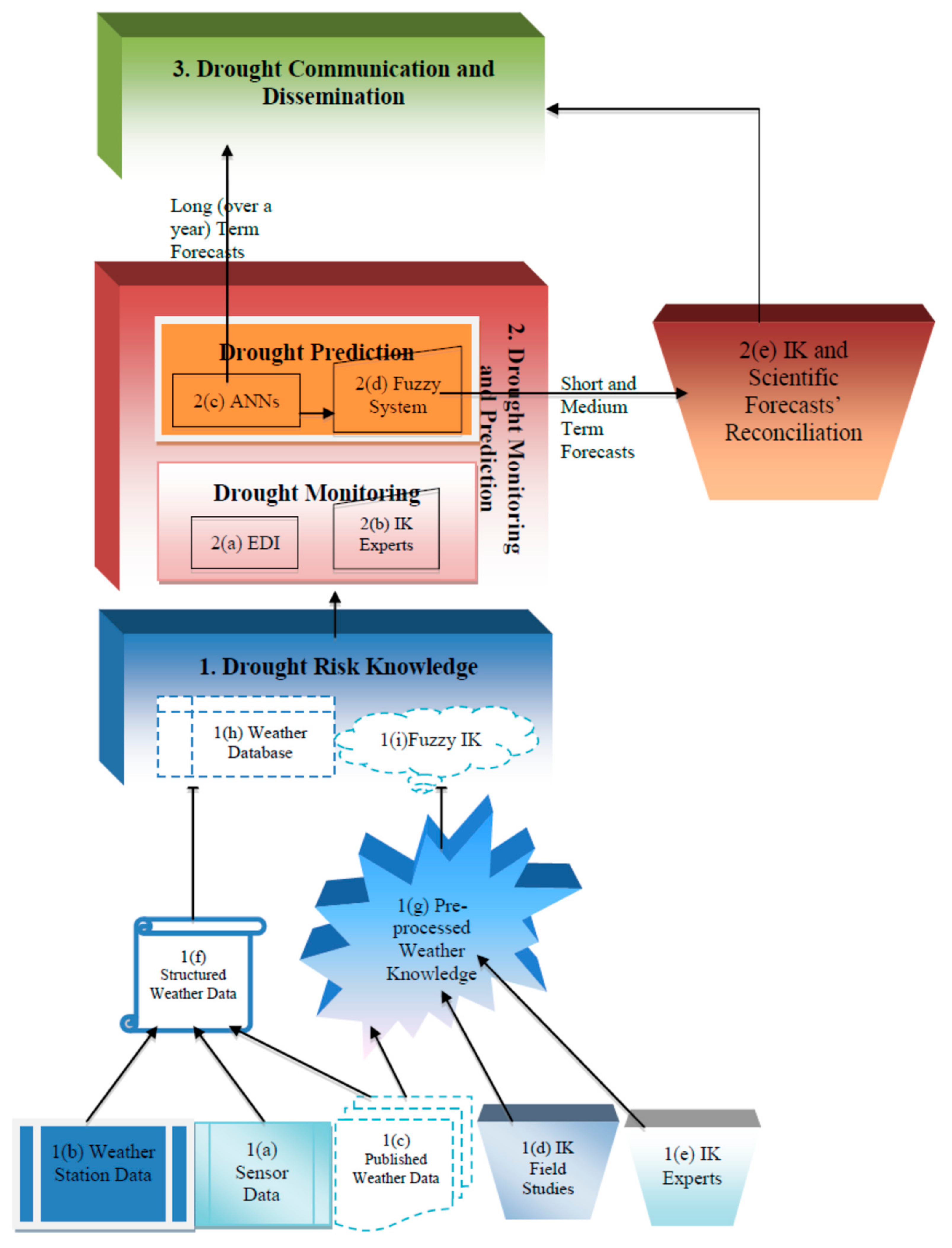
The main methodology followed in this research was the development of an integration framework. Information Technology and Indigenous Knowledge with Intelligence (ITIKI) is an integration framework that provides the blueprint for the implementation of a system that integrates SFCs with indigenous knowledge on droughts. The framework took the form of a generic early warning system (EWS) consisting of four components: (1) gathering of risk-related knowledge; (2) monitoring and predicting the situation; (3) communicating warning messages; and (4) responding to warnings [2]. However, the framework did not include element 4, which mostly requires resources and measures (for example, the distribution of relief food and planting materials) that are beyond the scope this research. In order to incorporate artificial intelligence, wireless sensor networks, mobile phones and IK in the 3-element EWS, the model was adapted as shown in Figure 4. Details of the framework (known as ĩtiki) were published in [18]. The main focus of the current paper is the formal representation of IK using FCMs.
2.3. Layer 1: Drought Knowledge
As described in Section 2.1 above, capturing the IK aspect of the drought knowledge was accomplished through three case studies in Kenya (Mbeere, Nganyi, and Taita), one in South Africa (Zulu people) and one in Mozambique (Ndau people). Scientific weather data was captured from sensor-based weather meters, conventional weather stations run by national meteorological organizations and historical weather data [18].
2.4. Layer 2: Drought Monitoring and Prediction
The monitoring and predication component was implemented using two subcomponents: (1) drought monitoring and (2) drought prediction. Drought monitoring pre-processed the data to detect suggestive patterns as well minimizing duplicates and other errors. This was achieved through effective drought index (EDI) monitor and Indigenous Knowledge (IK) experts. The IK experts made use of a mobile application to capture IK indicators. Drought prediction was done through Artificial Neural Network (ANN) and fuzzy logic system models [6].
2.4.1. Drought Monitoring Using the Effective Drought Index (EDI)
As shown in Figure 4, implementation of drought monitoring entails the integration of indigenous and scientific approaches. For the scientific drought monitoring part, the Effective Drought Index (EDI) was used.
Ref. [57] developed the Effective Drought Index (EDI) to address the Standardized Precipitation Index (SPI) shortcomings. EDI is different from SPI in a number of ways, one being that it is capable of calculating drought on a daily basis. In this research, the interest was microlevel drought indicators, and therefore, EDI was selected. EDI was also chosen because it is the only index that quantifies droughts in absolute terms. Firstly, it is possible to tell when the droughts start and end as well as the severity and the spatial distribution of the droughts. Other desirable features of EDI are as follows: (1) It calculates daily drought severity; (2) it calculates the current level of available water resources more accurately; (3) it considers drought continuity, not just a limited period—it can therefore diagnose prolonged droughts that continue for several years; (4) it is computed using precipitation alone; and (5) it considers daily water accumulation with a weighting function for time passage.
Calculation of EDI is made with consideration of the fact that the quantity of rainfall that can be used as a water resource drops gradually over time after the rain has fallen. Precipitation (EP) is used to compute the deficiency or surplus of water resources for a particular date and place. EP here refers to the summed value of daily precipitation with a time-dependent reduction function; it makes use of Equation (2) below.
where Pm is the precipitation of m days before, and the index, i, represents the duration of summation (DS) in days. Here, i = 365 is used; that is, the summation for a year which is the most dominant precipitation cycle worldwide. The value, 365, can then representative of the total water resources available or stored for a long time.
Using 30-year historical daily precipitation data, both monthly and daily EDI values for each of the locations that were considered in the case studies were computed and stored. EDI computes the ‘normal’ monthly precipitation for each calendar month of the year based on the mean precipitation of a calendar month for all 31 years (of historical data). For example,
The normal precipitation for November is the mean of the precipitations for November 1979, November 1980, November 28, 1980, …, November 2009.
The ‘normal’ precipitation for November in Mbeere may not be compared with the ‘normal’ precipitation for November for KwaZulu Natal, since the two are in different climatic zones. The EDI values solve this by use of standard deviations to compute universal real values that have a similar meaning in all climatic zones. Therefore, an EDI value of −2.59 will represent ‘Extreme Drought’ irrespective of climatic zone.
EDI applies a time-dependent reduction function in computing the monthly/daily water deficiency. This is to cater for runoff and evapotranspiration that progressively reduce soil moisture over time. The Available Water Resources Index (AWRI) expresses the actual amount of available water [58]. In order to visualize a drought in terms of classes, described by [57], the classification in Table 2 below was adapted:
For integration (of IK and EDI) purposes, similar calculations were used to compute daily and monthly EDI values for the periods within which the IK data collection took place.
2.4.2. Drought Forecasting: Artificial Neural Networks (ANNs)
Artificial Neural Network (ANN) models for each location were created by combining various inputs/targets extracted from the outputs (EDI and AWRI) of the EDI computations [6]. The lead-time (in days) considered included 1, 2, 3, 4, 5, 6, 7, 12 and 14. Given a specific day, n, to forecast an EDI or AWRI value for d days from n, the following expression was used:
Forecast [En+d] = f(En, En−1, En−2, En−3, En−4, En−5), where Ei is the EDI value for day i; the latter ranges from 1 to 6. That is, in order to forecast future values, six past values were input into the neural network. In case of AWRI, E was replaced with W. For example, to forecast the value of EDI with 5 days lead-time from 21 January to 26 January, the following expression was applied:
Forecast [E21+5] = f (E21, E20, E19, E18, E17, E16)
These models were then implemented in MATLAB’s Neural Network Toolbox, leading to drought prediction accuracies ranging from 75% to 98%. The accuracies were determined using a combination of percent Root Mean Square Error (%RMSE) and Regression (R).
2.4.3. Drought Forecasting: Fuzzy System
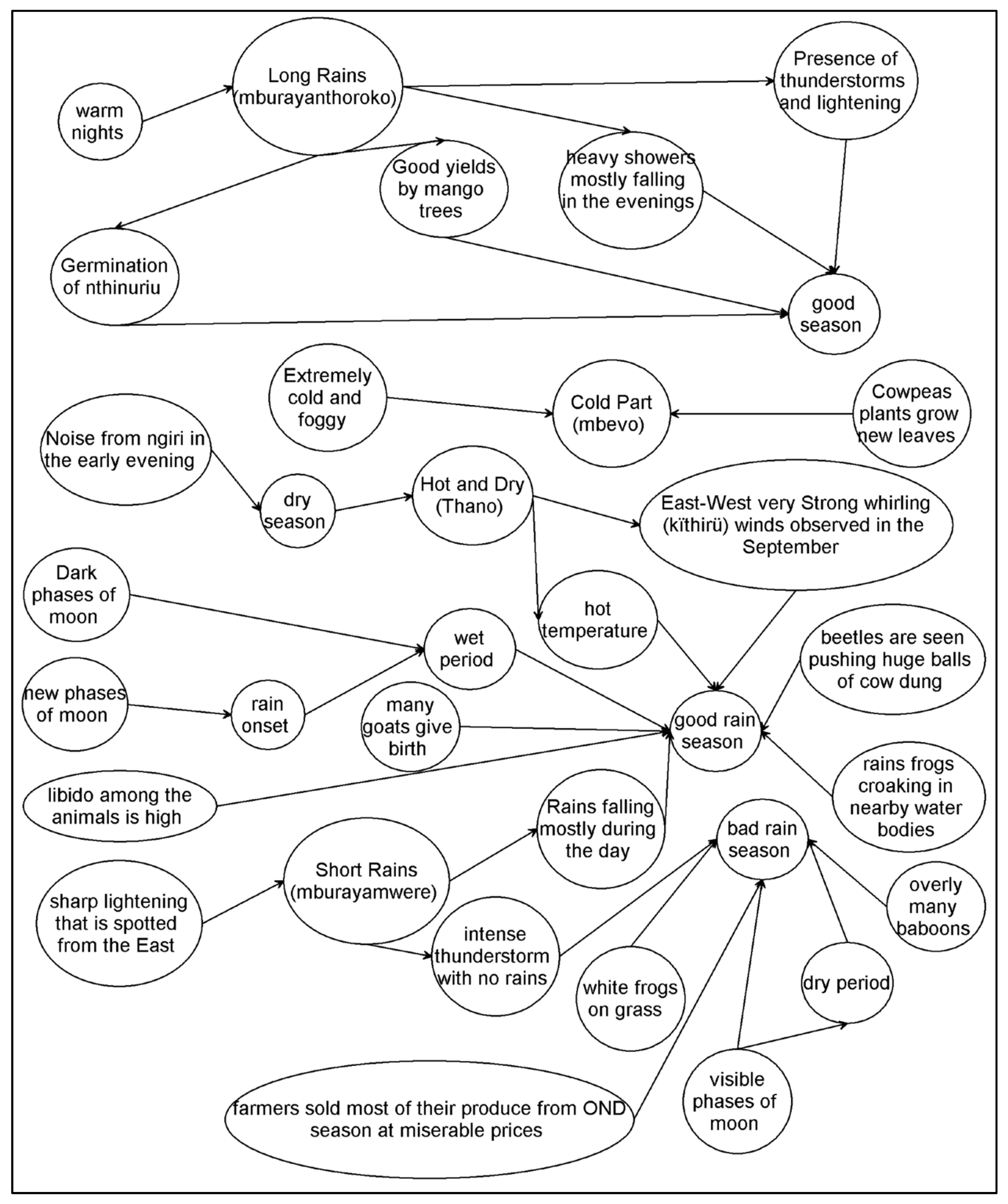
FCMs were generated for each of the case studies. In most cases, a network of more than one FCM was generated in order to capture all of the indicators and their causal effects. The FCM in Figure 5, for example, captures indicators for the Mbeere people.
One set of indicators, representing one season, was then selected for further modelling. Using this set, a simple form of learning was characterized by aggregating knowledge from corresponding seasonal fuzzy cognitive map matrices into single units. This was done by adding the adjacent matrices of the seasonal FCM, , to form an overall FCM connection matrix, . The resultant matrix had values outside the range [−1, 1]; hence, for scaling, the combined matrix was divided by N.
The object, , represented the overall seasonal FCM, corresponds to the number of FCMs, and corresponds to the FCM connection matrix of the season. The final fuzzy cognitive map connection matrices consisted of collective knowledge for all seasons for each case study.
The causal effects between the concepts (weather indicators) were declared using the variable “causal effect” which uses values, w, in a closed range, −1 ≤ w ≤ 1, with term sets, T, that are proposed to comprise five linguistic variables representing the different degrees of causal effects between concept(s).
T (causal effect) = {strong positive, positive, none, negative, strong negative}, using the range of strong positive to strong negative effects, as follows:
0.5 < strong_positive ≤ 1
0 < positive ≤ 0.5
0 = none
0.5 < negative < 0
−1 < strong_negative < −0.5
The densities, D, of the seasonal fuzzy cognitive maps were determined to depict how highly connected the concepts are to each other. For each seasonal fuzzy cognitive map, the densities were computed by dividing the number of countable connections, Z, by the number of possible connections between N concepts. Given that the relationships between the seasonal connection matrices depicted no self-loops, the main diagonal of the connection matrices consisted only of zeros. The maximum number of concepts connections was given by N (N − 1). The densities in the seasonal fuzzy cognitive maps were determined by
The implementation significance of density was that seasonal fuzzy cognitive maps with many connections per concept had higher densities, provided by increased alternatives for manipulating the IK concepts. The in degrees were computed by summing the counts of all of the absolute values of incident arrows. In the connection matrices, this was the sum of the columnar IK concepts. The out degrees were determined by summing the counts of all of the absolute values of the outgoing arrows. In the connection matrices, this was the sum of the row IK concepts. The absolute values were used to give equal importance to recognize both negative and positive causal effect weights between IK concepts.
The centralities of all of the IK concepts for each seasonal fuzzy cognitive map were determined. The centrality was also called the total degree of the IK concepts (i.e., the sum of the in degree and out degree per IK concept). The centrality was used to measure the importance of the IK concepts; IK concepts with high centrality were given special attention.
3. Results
3.1. Integrated Drought Early Warning System
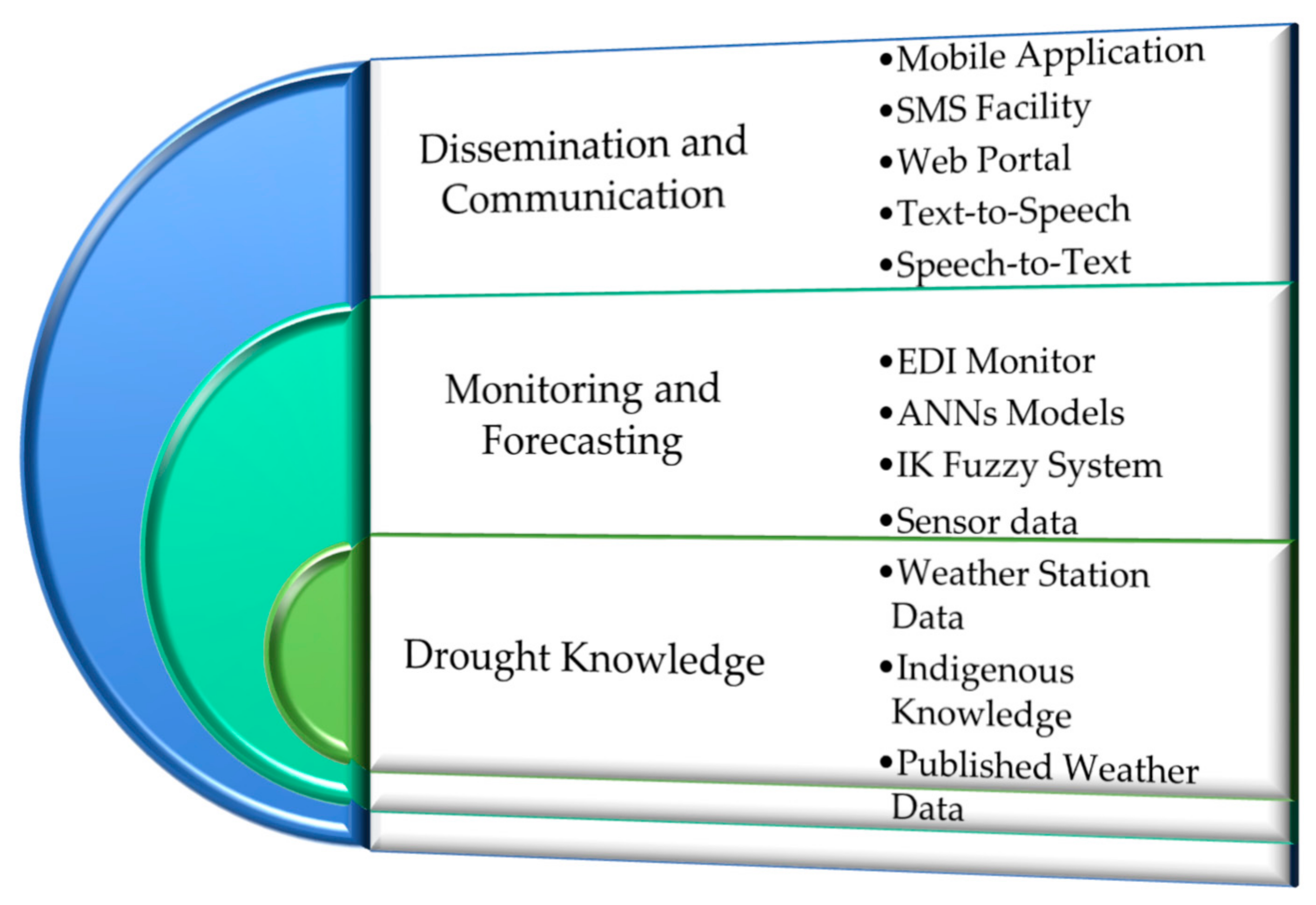
The integration framework was realized in the form of a three-layered drought early warning system prototype: a drought knowledge capture layer, a drought monitoring and predication layer and finally, drought forecast dissemination and communication (see Figure 6).
3.1.1. Drought Knowledge
Data from sensors was sent to a central database via a Java-based Short Message Service (SMS) gateway. Weather station data and indigenous knowledge were captured into the system via a web interface and a mobile phone application, respectively. Forecasts were automatically retrieved from published weather data from meteorological organizations’ (Kenya Meteorological Department and the South Africa Weather Service) weather reports.
3.1.2. Monitoring and Forecasting
The data collected and stored in the drought knowledge layer was used by the following three subsystems:
- (a)
- The EDI monitor that handled the ‘monitoring’ aspect. Here, the stand-alone FORTRAN program developed by [57] was used.
- (b)
- Artificial Neural Networks (ANNs) were in charge of the ‘forecasting’ aspect. These were implemented in MATLAB and used to predict future values (EDI and AWRI) of droughts.
- (c)
- A Fuzzy Logic System handled the monitoring and forecasting of droughts using indigenous knowledge. This was also implemented using MATLAB; its output was uploaded to the MySQL database from where it was linked to the ANN models’ output.
3.1.3. Dissemination and Communication
The system is accessible to end users via five input/output channels: (1) a mobile application that is used for inputting and outputting IK indicators and extreme weather events; (2) an SMS facility for requesting drought and weather forecasts as well as for extreme weather events alerts; (3) a web portal which is used to access comprehensive information on droughts, weather and extreme events. The formats available include text, graphs and audio files; (4) Text-to-speech is a simple plug-in implemented to generate audio formats of the drought and weather forecasts; and (5) speech-to-text which is also a plug-in for android phones that is used as an alternative to typing input data via the android application.
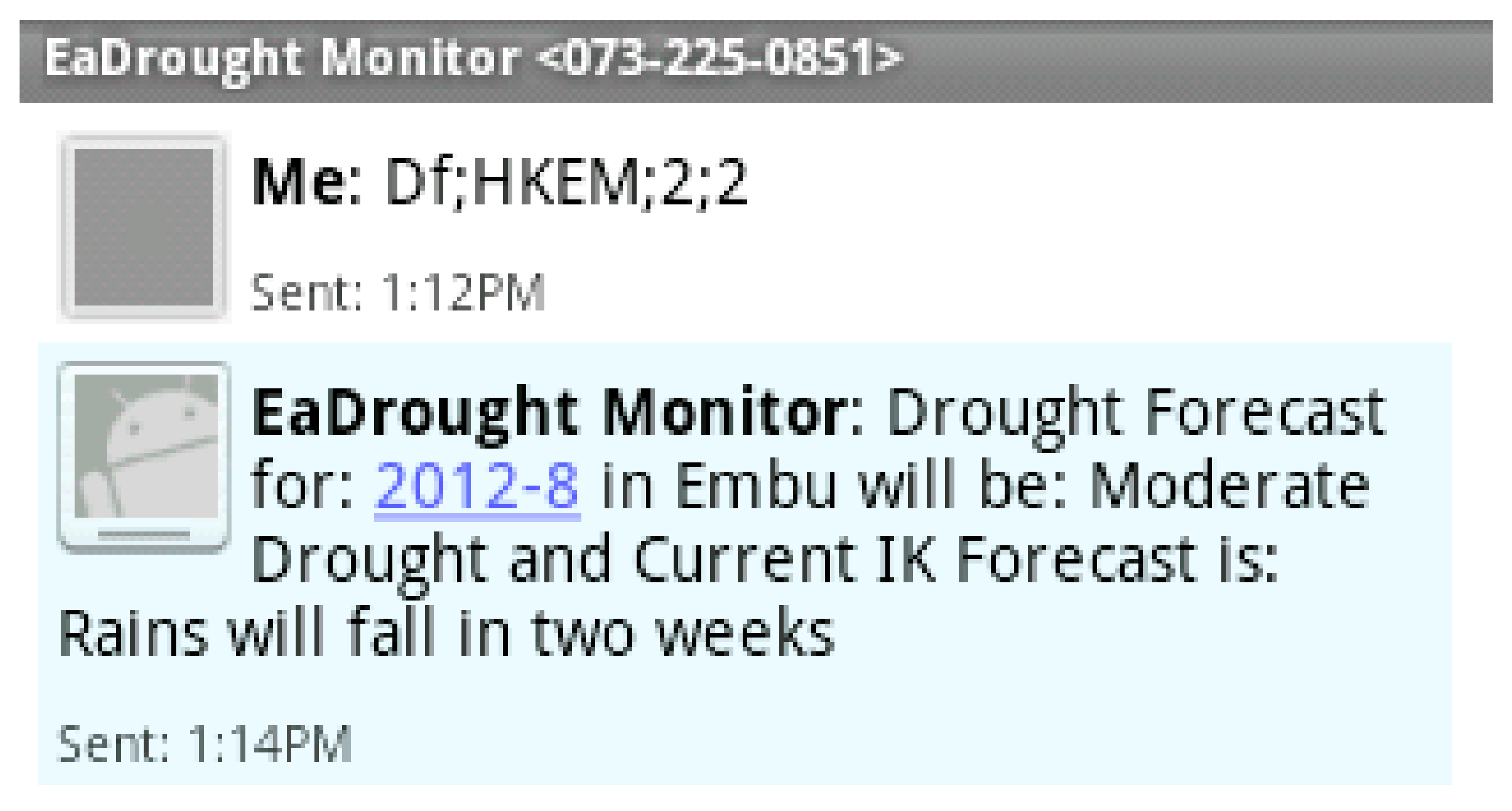
An SMS request to the Medium-Term Drought for Embu (this serves Mbeere region) weather station for two months lead time generated some output (see Figure 7):
3.2. EDI Monitor
The EDI computer program’s [57] NAMELIST.TXT file was edited to accommodate inputs related to the case studies considered. See Figure 8, where data for a station named “District 83” is used as the input to the EDI program.
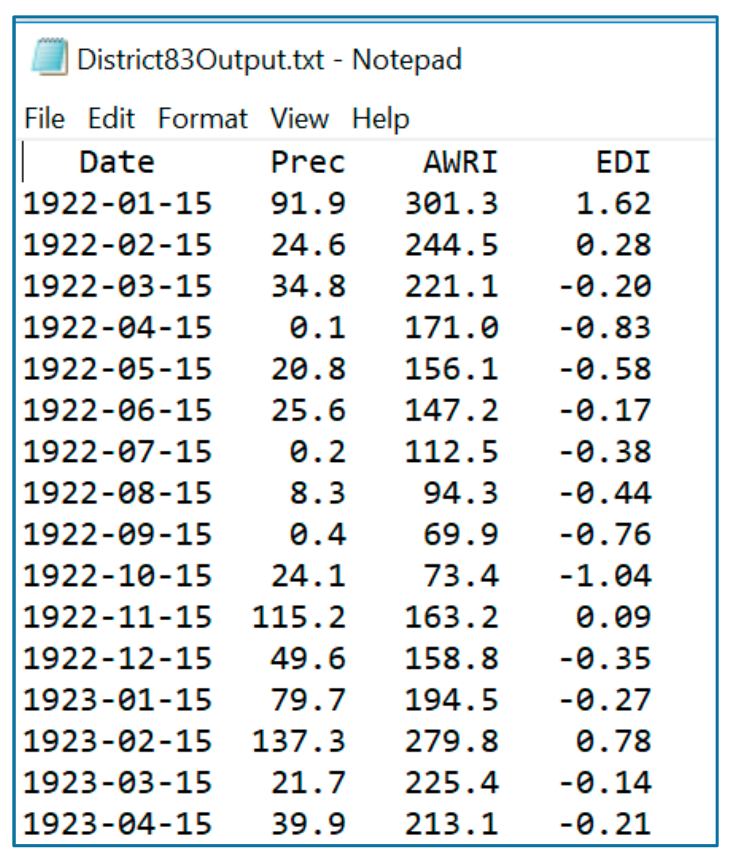
Upon execution, an output file for each of the location was realized, each showing the EDI and AWRI, as shown in the example in Figure 9.
In Table 3, the AWRI for December 1980 was 460.8. A total of 14.9 mm of precipitation was received in January 1981. Simple summation of monthly precipitation would have yielded 475.7, but factoring in runoff and evapotranspiration EDI yielded 364.2.
3.3. IK Fuzzy Logic System
The IK Fuzzy Logic System handled the knowledge management, monitoring and forecasting of droughts using indigenous knowledge. Each fuzzy cognitive map generated the actual weights of the causal effects, represented in the form of tables (see Table 4 and Table 5).
Table 6 is an example of determination of the importance of the IK concepts for the spring season.
4. Conclusions and Further Work
In this research, a method was developed to formally represent indigenous knowledge as used by traditional communities to predict droughts. In this method, fuzzy cognitive mapping was used to model and represent causal relationships between selected indigenous knowledge and weather conditions. The indigenous knowledge used to generate FCM maps was collected through case studies of five communities in Kenya, Mozambique and South Africa.
The case studies were important in understanding the indigenous knowledge domain as well as linking the causal effects between indigenous knowledge and weather/drought indicators. The representations made it possible to match IK indicators with associated drought/weather conditions through weighted graphs.
The FCMs were represented in the form of matrices with relationships between the weather concepts. A number of transformation functions were devised, leading to a fuzzy system capable of generating drought predications given a set of IK indicators. The output from the fuzzy system was formal (quantitative) enough to be integrated with the values (EDI values) generated from artificial neural network drought prediction models.
The predicted outcomes were also enhanced by integrating iterative reorganization (a simple form of learning) of the season connection matrix weights before successive steps of a simulation. The prediction component portrayed the uncertainty of the seasons by allowing the choice of specification of the weather season and status; otherwise, mechanisms were put in place for the model to utilize object time stamps for season resolution.
Both the EDI and AWRI values generated from the ANN drought predication subsystems and the results from the fuzzy system were integrated and disseminated to the users. This is partially a manual activity in which the meteorologists and the IK experts reconcile the results from the two knowledge systems. However, the short-term forecasts (a few hours to two weeks) do not need the manual ‘reconciliation’, because the system intelligently reconciles the two (from IK and from ANNs) and sends them to the drought communication and dissemination component. Further, in line with fuzzy system, for purposes of ‘recovering’ IK’s original meaning/format, the output from the fuzzy system is passed through a defuzzification process.
Implementation of the integration framework is in prototype form. More work, aimed at converting it into a fully functional drought predication system is needed. However, our formal representation of the IK contributes to the missing link—scientific validation and verification of the IK.
Acknowledgments
The authors thank the two anonymous reviewers for their valuable comments.
Author Contributions
Muthoni Masinde and Mwanjele Mwagha conceived and designed the experiments, performed the experiments, and analyzed the data; Tsegaye Tadesse contributed reagents/materials/analysis tools; All the authors drafted and refined the paper. In terms of data and methods, Muthoni Masinde collected and analyzed data for three of the case studies while Mwanjele Mwagha was responsible for the other two. All the three authors drafted and refined this paper.
Conflicts of Interest
The authors declare no conflict of interest.
Appendix A
Extract from the IK Data Collection Interview Guide

References
- Wilhite, D.A.; Glantz, M.H. Understanding the Drought Phenomenon: The Role of Definitions. Water Int. 1985, 10, 111–120. [Google Scholar] [CrossRef]
- ISDR; ECA; UNDP. 3rd African Drought Adaptation Forum Report September, 2008; ISDR, ECA, UNDP: Addis Ababa, Ethiopia, 2008. [Google Scholar]
- Zwaagstra, L.; Sharif, Z.; Wambile, A.; Leeuw, J.D.; Said, M.Y.; Johnson, N.; Njuki, J.; Ericksen, P.; Herrero, M. An Assessment of the Response to the 2008–2009 Drought in Kenya. Available online: https://cgspace.cgiar.org/bitstream/handle/10568/2057/assessment_drought_2010.pdf?sequence=3 (accessed on 10 November 2017).
- Morid, S.; Smakhtin, V.; Bagherzadeh, K. Drought forecasting using artificial neural networks and time series of drought indices. Int. J. Climatol. 2007, 27, 2103–2111. [Google Scholar] [CrossRef]
- Trenberth, K.E.; Branstator, G.W.; Karoly, D.; Kumar, A.; Lau, N.C.; Ropelewski, C. Progress during TOGA in understanding and modeling global teleconnections associated with tropical sea surface temperatures. J. Geophys. Res. Oceans 1998, 103, 14291–14324. [Google Scholar] [CrossRef]
- Masinde, M. Artificial neural networks models for predicting effective drought index: Factoring effects of rainfall variability. Mitig. Adapt. Strat. Glob. Chang. 2014, 19, 1139–1162. [Google Scholar] [CrossRef]
- Marshall, N.A.; Gordon, I.J.; Ash, A.J. The reluctance of resource-users to adopt seasonal climate forecasts to enhance resilience to climate variability on the rangelands. Clim. Chang. 2011, 107, 511–529. [Google Scholar] [CrossRef]
- Mwagha, S.M.; Masinde, M. Scientific Verification of Weather Lore for Drought Forecasting—The Role of Fuzzy Cognitive Mapping. In Proceedings of the IST-Africa 2015 Conference, Lilongwe, Malawi, 6–8 May 2015; Cunningham, P., Cunningham, M., Eds.; IIMC International Information Management Corporation: Dublin, Ireland, 2015. ISBN 978-1-905824-50-2. [Google Scholar]
- Mugabe, F.T.; Mubaya, C.P.; Nanja, D.; Gondwe, P.; Munodawafa, A.; Mutswangwa, E.; Chagonda, I.; Masere, P.; Dimes, J.; Murewi, C. Use of Indigenous Knowledge Systems and Scientific Methods for Climate Forecasting in Southern Zambia and North-Western Zimbabwe. Zimb. J. Technol. Sci. 2010, 1, 19–30. [Google Scholar] [CrossRef]
- Ziervogel, G.; Bithell, M.; Washington, R.; Downing, T. Agent-based social simulation: A method for assessing the impact of seasonal climate forecast applications among smallholder farmers. Agric. Syst. 2005, 83, 1–26. [Google Scholar] [CrossRef]
- Enock, C.M. Indigenous Knowledge Systems and Modern Weather Forecasting: Exploring the Linkages. J. Agric. Sustain. 2013, 2, 98–141. [Google Scholar]
- Anandaraja, N.; Rathakrishnan, T. Indigenous weather and forecast practices of Coimbatore district farmers of Tamil Nadu. Indian J. Tradit. Knowl. 2008, 7, 630–633. [Google Scholar]
- Masinde, M.; Bagula, A. ITIKI: Bridge between African indigenous knowledge and modern science of drought prediction. Knowl. Manag. Dev. J. 2011, 7, 274–290. [Google Scholar] [CrossRef]
- Warren, D.M. Information and Communication Technologies, Knowledge Management and Indigenous Knowledge: Implications to Livelihood of Communities in Ethiopia; World Bank Discussion Paper 127; The World Bank: Washington, DC, USA, 1991; pp. 1–12. [Google Scholar]
- Risiro, J.; Mashoko, D.; Tshuma, T.; Rurinda, E. Weather Forecasting and Indigenous Knowledge Systems in Chimanimani District of Manicaland. Zimb. J. Emerg. Trends Educ. Res. Policy Stud. 2012, 3, 561–566. [Google Scholar]
- Xue, S. Neural Fuzzy Inference System-Based Weather Prediction Model and Its Precipitation Predicting Experiment. Atmosphere 2014, 5, 788–805. [Google Scholar] [CrossRef]
- Ziervogel, G.; Downing, T.E. Stakeholder networks: improving seasonal climate forecasts. Clim. Chang. 2004, 65, 73–101. [Google Scholar] [CrossRef]
- Masinde, M. An innovative drought early warning system for sub-Saharan Africa: Integrating modern and indigenous approaches. Afr. J. Sci. Technol. Innov. Dev. 2015, 7, 8–25. [Google Scholar] [CrossRef]
- Mercer, J.; Kelman, I.; Taranis, L.; Suchet-Pearson, S. Framework for integrating indigenous and scientific knowledge for disaster risk reduction. Disasters 2010, 34, 214–239. [Google Scholar] [CrossRef] [PubMed]
- Roncoli, C. Ethnographic and participatory approaches to research on farmers’ responses to climate predictions. Clim. Res. 2006, 33, 81. [Google Scholar] [CrossRef]
- Stigter, C.J.; Dawei, Z.; Onyewotu, L.O.Z.; Xurong, M. Using traditional methods and indigenous technologies for coping with climate variability. Clim. Chang. 2005, 70, 255–271. [Google Scholar] [CrossRef]
- Brokensha, D.W.; Warren, D.M.; Werner, O. Indigenous Knowledge Systems and Development; University Press of America: Lanham, MD, USA, 1980. [Google Scholar]
- Flora, C.B. Reconstructing agriculture: The case for local knowledge. Rural Sociol. 1992, 57, 92–97. [Google Scholar] [CrossRef]
- Sillitoe, P. The development of indigenous knowledge: A new applied anthropology 1. Curr. Anthropol. 1998, 39, 223–252. [Google Scholar] [CrossRef] [Green Version]
- Thrupp, L.A. Legitimizing local knowledge: From displacement to empowerment for Third World people. Agric. Hum. Values 1989, 6, 13–24. [Google Scholar] [CrossRef]
- Virji, H.; Cory, F.; Amy, F.; Mayuri, S. Climate Variability, Water Resources and Agricultural Productivity: Food Security Issues in Tropical Sub-Saharan Africa; World Food Programme: Rome, Italy, 1997. [Google Scholar]
- Krupnik, I.; Ray, G.C. Pacific walruses, indigenous hunters, and climate change: Bridging scientific and indigenous knowledge. Deep Sea Res. Part II Top. Stud. Oceanogr. 2007, 54, 2946–2957. [Google Scholar] [CrossRef]
- Lauer, M.; Aswani, S. Integrating indigenous ecological knowledge and multi-spectral image classification for marine habitat mapping in Oceania. Ocean Coast. Manag. 2008, 51, 495–504. [Google Scholar] [CrossRef]
- Voinov, A.; Bousquet, F. Modelling with stakeholders. Environ. Modell. Softw. 2010, 25, 1268–1281. [Google Scholar] [CrossRef]
- Voinov, A.; Gaddis, E.J.B. Lessons for successful participatory watershed modelling: A perspective from modeling practitioners. Ecol. Model. 2008, 216, 197–207. [Google Scholar] [CrossRef]
- Giordano, R.; Liersch, S. A fuzzy GIS-based system to integrate local and technical knowledge in soil salinity monitoring. Environ. Model. Softw. 2012, 36, 49–63. [Google Scholar] [CrossRef]
- Sicat, R.S.; Carranza, E.J.M.; Nidumolu, U.B. Fuzzy modeling of farmers’ knowledge for land suitability classification. Agric. Syst. 2005, 83, 49–75. [Google Scholar] [CrossRef]
- Zadeh, L.A. Fuzzy sets. Inf. Control 1965, 8, 338–353. [Google Scholar] [CrossRef]
- Kosko, B. Fuzzy Cognitive Maps. Int. J. Man-Mach. Stud. 1986, 24, 65–75. [Google Scholar] [CrossRef]
- Maitra, S.; Banerjee, D. Application of Fuzzy Cognitive Mapping for Cognitive Task Analysis in Mechanised Mines. IOSR J. Mech. Civ. Eng. 2014, 11, 20–28. [Google Scholar] [CrossRef]
- Chinlampianga, M. Traditional knowledge, weather prediction and bioindicators: A case study in Mizoram, Northeastern India. Indian J. Tradit. Knowl. 2011, 10, 207–211. [Google Scholar]
- Guerram, T.; Maamri, R.; Sahnoun, Z. A Tool for Qualitative Causal Reasoning on Complex Systems. Int. J. Comput. Sci. Issues 2010, 7, 120–125. [Google Scholar]
- Mago, V.K.; Morden, H.K.; Fritz, C.; Wu, T.; Namazi, S.; Geranmayeh, P. Analyzing the impact of social factors on homelessness: A Fuzzy Cognitive Map approach. BMC Med. Inform. Decis. Mak. 2013, 13, 1–19. [Google Scholar] [CrossRef] [PubMed]
- Xirogiannis, G.; Glykas, M. Fuzzy Cognitive Maps in Business Analysis and Performance-Driven Change. IEEE Trans. Eng. Manag. 2004, 51, 334–351. [Google Scholar] [CrossRef]
- Chrysostomos, S.; Peter, G. Mathematical Formulation of Fuzzy Cognitive Maps. In Proceedings of the 7th Mediterranean Conference on Control and Automation, Haifa, Israel, 28–30 June 1999; pp. 2251–2261. [Google Scholar]
- Karagiannis, I.; Groumpos, P. Input-Sensitive Fuzzy Cognitive Maps. Int. J. Comput. Sci. Issues 2013, 10, 143–151. [Google Scholar]
- Carvalho, J.P. On the Semantics and the Use of Fuzzy Cognitive Maps in Social Sciences. In Proceedings of the 2010 IEEE World Congress on Computational Intellige nce (WCCI), Barcelona, Spain, 18–23 July 2010; pp. 18–23. [Google Scholar]
- Chrysafiadi, K.; Virvou, M. A knowledge representation approach using fuzzy cognitive maps for better navigation support in an adaptive learning system. Springerplus 2013, 2, 81. [Google Scholar] [CrossRef] [PubMed]
- Din, M.A.; Cretan, G.C. Causal modelling of the higher education determinants regarding the labour market absorption of graduates: A Fuzzy Cognitive Maps approach. Int. J. Fuzzy Syst. Adv. Appl. 2014, 1, 1–6. [Google Scholar]
- Yousef, O.M.S. Causality analysis of the technology strategy maps using the fuzzy cognitive strategy map. Afr. J. Bus. Manag. 2014, 8, 191–210. [Google Scholar] [CrossRef]
- Aguilar, J. A Survey about Fuzzy Cognitive Maps Papers. Int. J. Comput. Cognit. 2005, 3, 27–33. [Google Scholar]
- Papageorgiou, E.; Kontogianni, A. Using Fuzzy Cognitive Mapping in Environmental Decision Making and Management: A Methodological Primer and an Application. In International Perspectives on Global Environmental Change; Young, S., Ed.; InTech: London, UK, 2012; pp. 427–450. ISBN 978-953-307-815-1. Available online: http://www.intechopen.com/books/international-perspectives-on-global-environmental-change/using-fuzzy-cognitive-mapping-in-environmental-decision-making-and-management-a-methodological-prime (accessed on 10 November 2017).
- Văidianu, M.N. Fuzzy cognitive maps: Diagnosis and scenarios for a better management process of visitors flows in Romanian Danube Delta Biosphere Reserve. J. Coast. Res. 2013, 65, 1063–1068. [Google Scholar] [CrossRef]
- Kwon, S.J.; Mustapha, E.E. Exploring the Effect of Cognitive Map on Decision Makers’ Perceived Equivocality and Usefulness in the Context of Task Analyzability and Representation. In Proceedings of the Fifth International Conference on Information, Process, and Knowledge Management, Nice, France, 24 February–1 March 2013; pp. 117–122. [Google Scholar]
- Rangarajan, K.; Jayasudha, S.; Ramanathan, K. Fuzzy Petri Nets and Fuzzy Cognitive Maps. Int. J. Comput. Appl. 2012, 46, 5–9. [Google Scholar]
- Orlove, B.; Roncoli, C.; Merit, K.; Abushen, M. Indigenous climate knowledge in southern Uganda: The multiple components of a dynamic regional system. Clim. Chang. 2009, 100, 243–265. [Google Scholar] [CrossRef]
- Morton, J.; Barton, D.; Collinson, C.; Heath, B. Comparing Drought Mitigation Interventions in the Pastoral Livestock Sector; University of Greenwich, Natural Resource Institute: Chatham, UK, 2006. [Google Scholar]
- The Arid Lands Resource Management Project (ALRMP). Wajir District Vision and Strategy: 2005–2015; Government of Kenya: Nairobi, Kenya, 2005.
- The Kenya Census 2009: Population and Housing Census Highlights. Available online: https://www.knbs.or.ke/2009-kenya-population-and-housing-census-analytical-reports/ (accessed on 10 November 2017).
- Duan, N.; Hoagwood, K. Purposeful Sampling for Qualitative Data Collection and Analysis in Mixed Method Implementation Research. Adm. Policy Ment. Health Serv. Res. 2015, 42, 533–544. [Google Scholar] [CrossRef]
- Preist, C.; Massung, E.; Coyle, D. Competing or aiming to be average?: Normification as a means of engaging digital volunteers. In Proceedings of the 17th ACM Conference on Computer Supported Cooperative Work and Social Computing, Baltimore, MD, USA, 15–19 February 2014; pp. 1222–1233. [Google Scholar]
- Byun, H.; Wilhite, D.A. Objective quantification of drought severity and duration. J. Clim. 1999, 12, 2747–2756. [Google Scholar] [CrossRef]
- Wilhite, D.A.; Svoboda, M.D. Drought Early Warning Systems in the Context of Drought Preparedness and Mitigation; World Meteorological Organization: Geneva, Switzerland, 2000; pp. 1–16. [Google Scholar]
Figure 1.
Depiction of fuzzy cognitive mapping (FCM).

Figure 2.
Depiction a FCM showing influence between indigenous knowledge (IK) concepts.

Figure 3.
Locations of the case studies in Kenya, Mozambique and South Africa.

Figure 4.
ITIKI: Integrated Drought Early Warning System Framework.

Figure 5.
An FCM showing causal relationships among IK concepts for Mbeere.

Figure 6.
Architecture of ITIKI implementation.

Figure 7.
Medium Term Drought Forecast—SMS.

Figure 8.
Sample input file parameters for the EDI program.
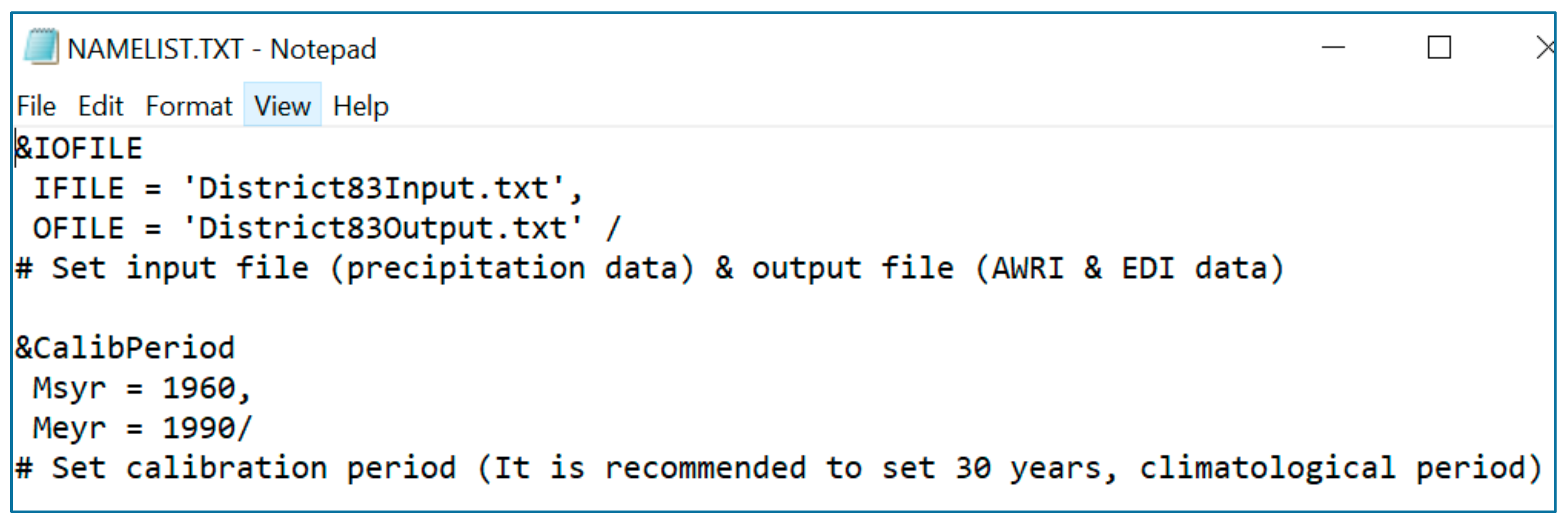
Figure 9.
Sample input file for the EDI program.


Table 1.
Characteristics of Weather Seasons in KwaZulu-Natal.
| Season | Local Name | Onset Signs | Cessation Signs |
|---|---|---|---|
| Summer | Ihlobo (October–February) | Lightening Very hot Daytime rain | Cold Winds Temperature lowers Rain stops |
| Autumn | Intwasabusika (March–May) | Trees shed leaves Grass changes color | Very cold |
| Winter | Ubusika (May–July) | Mists | Clear sky in the morning Birds build new nests Trees look dry |
| Spring | Intwasahlo (August–October) | Lots of wind | Very hot |
Table 2.
Effective Drought Index (EDI) classification [57].
Table 2.
Effective Drought Index (EDI) classification [57].
| Drought Class Description | Drought Index Values |
|---|---|
| Extreme Flood | EDI > 2 |
| Severe Flood | 1.5 < EDI < 1.99 |
| Moderate Flood | 1 < EDI < 1.49 |
| Wet–Near Normal | 0.01 < EDI < 0.99 |
| Drought–Near Normal | −0.99 < EDI < 0.00 |
| Moderate Drought | −1 < EDI < −1.49 |
| Severe Drought | −1.5 < EDI < −1.99 |
| Extreme Drought | EDI < −2 |
Table 3.
Monthly EDI Output File Format.
| Date | Total Precipitation | AWRI | EDI |
|---|---|---|---|
| 15 June 1980 | 70.80 | 230.0 | −0.51 |
| 15 February 1980 | 13.0 | 179.7 | −0.65 |
| 15 March 1980 | 37.9 | 170.1 | −0.86 |
| 15 April 1980 | 105.9 | 229.8 | −1.35 |
| 15 December 1980 | 33.5 | 460.8 | 1.05 |
| 15 June 1981 | 14.6 | 364.9 | 0.37 |
| 15 December 2009 | 121.10 | 297.5 | −0.27 |
KEY: AWRI–Available Water Resource Index; EDI–Effective Drought Index.
Table 4.
Depiction of Fuzzy Cognitive Map for Winter Season.
| Concepts | High Clouds | Low Clouds | Medium Clouds | Clear Sky | Many Stars | Rainbow | Lightning | Partial/Dark Moon | Full/Visible Moon | Rain | Dry | Hot | Cold |
|---|---|---|---|---|---|---|---|---|---|---|---|---|---|
| High clouds | 0.00 | 0.00 | 0.00 | 0.50 | 0.00 | 0.00 | −1.00 | 0.00 | 0.00 | −0.75 | 0.75 | 0.75 | −1.00 |
| Low clouds | 0.00 | 0.00 | 0.00 | −1.00 | 0.00 | 0.00 | 0.00 | 0.00 | 0.00 | 0.50 | 0.00 | −0.50 | 0.50 |
| Medium clouds | 0.00 | 0.00 | 0.00 | −0.50 | 0.00 | 0.00 | 0.00 | 0.00 | −0.50 | 0.00 | 0.00 | 0.00 | 0.50 |
| Clear sky | 0.00 | 0.00 | 0.00 | 0.00 | 0.00 | 0.00 | −1.00 | 0.00 | 0.00 | −0.75 | 0.75 | 1.00 | −1.00 |
| Many stars | 0.00 | 0.00 | 0.00 | 0.00 | 0.00 | 0.00 | 0.00 | 0.00 | 0.00 | −1.00 | 0.75 | 0.75 | −1.00 |
| Rainbow | 0.00 | 0.00 | 0.00 | 0.00 | 0.00 | 0.00 | 0.00 | 0.00 | 0.00 | −0.50 | 0.00 | 0.50 | 0.00 |
| Lightning | 0.00 | 0.00 | 0.00 | 0.00 | 0.00 | 0.00 | 0.00 | 0.00 | 0.00 | 1.00 | −1.00 | −0.75 | 0.75 |
| Partial/dark moon | 0.00 | 0.00 | 0.00 | 0.00 | 0.00 | 0.00 | 0.00 | 0.00 | 0.00 | 0.50 | −0.75 | −0.50 | 0.50 |
| Full/visible moon | 0.00 | 0.00 | 0.00 | 0.00 | 0.00 | 0.00 | 0.00 | 0.00 | 0.00 | −0.75 | −0.25 | 0.75 | −0.75 |
| Rain | 0.00 | 0.00 | 0.00 | 0.00 | 0.00 | 0.00 | 0.00 | 0.00 | 0.00 | 0.00 | 0.00 | 0.00 | 0.00 |
| Dry | 0.00 | 0.00 | 0.00 | 0.00 | 0.00 | 0.00 | 0.00 | 0.00 | 0.00 | 0.00 | 0.00 | 0.00 | 0.00 |
| Hot | 0.00 | 0.00 | 0.00 | 0.00 | 0.00 | 0.00 | 0.00 | 0.00 | 0.00 | 0.00 | 0.00 | 0.00 | 0.00 |
| Cold | 0.00 | 0.00 | 0.00 | 0.00 | 0.00 | 0.00 | 0.00 | 0.00 | 0.00 | 0.00 | 0.00 | 0.00 | 0.00 |
Table 5.
Depiction of the Importance of Nodes (Concepts) for the Spring Season.
| Concepts | Out Degree | In Degree | Centrality |
|---|---|---|---|
| High clouds | 4.75 | 0.00 | 4.75 |
| Low clouds | 2.50 | 0.00 | 2.50 |
| Medium clouds | 1.50 | 0.00 | 1.50 |
| Clear sky | 4.50 | 2.00 | 6.50 |
| Many stars | 3.50 | 0.00 | 3.50 |
| Rainbow | 1.00 | 0.00 | 1.00 |
| Lightning | 3.50 | 2.00 | 5.50 |
| Partial/dark moon | 2.25 | 0.00 | 2.25 |
| Full/visible moon | 2.50 | 0.50 | 3.00 |
| Rain | 0.00 | 5.75 | 5.75 |
| Dry | 0.00 | 4.25 | 4.25 |
| Hot | 0.00 | 5.50 | 5.50 |
| Cold | 0.00 | 6.00 | 6.00 |
Table 6.
Spring Season Dynamics.
| Spring | C1 | C2 | C3 | C4 | C5 | C6 | C7 | C8 | C9 | C10 | C11 | C12 | C13 |
|---|---|---|---|---|---|---|---|---|---|---|---|---|---|
| In degree | 0 | 0 | 0 | 3 | 0 | 0 | 2 | 0 | 1 | 9 | 9 | 9 | 8 |
| Out degree | 6 | 5 | 6 | 5 | 4 | 4 | 4 | 3 | 4 | 0 | 0 | 0 | 0 |
| Centrality | 6 | 5 | 6 | 8 | 4 | 4 | 6 | 3 | 5 | 9 | 9 | 9 | 8 |
© 2018 by the authors. Licensee MDPI, Basel, Switzerland. This article is an open access article distributed under the terms and conditions of the Creative Commons Attribution (CC BY) license (http://creativecommons.org/licenses/by/4.0/).
Share and Cite
MDPI and ACS Style
Masinde, M.; Mwagha, M.; Tadesse, T. Downscaling Africa’s Drought Forecasts through Integration of Indigenous and Scientific Drought Forecasts Using Fuzzy Cognitive Maps. Geosciences 2018, 8, 135. https://doi.org/10.3390/geosciences8040135
AMA Style
Masinde M, Mwagha M, Tadesse T. Downscaling Africa’s Drought Forecasts through Integration of Indigenous and Scientific Drought Forecasts Using Fuzzy Cognitive Maps. Geosciences. 2018; 8(4):135. https://doi.org/10.3390/geosciences8040135
Chicago/Turabian StyleMasinde, Muthoni, Mwanjele Mwagha, and Tsegaye Tadesse. 2018. "Downscaling Africa’s Drought Forecasts through Integration of Indigenous and Scientific Drought Forecasts Using Fuzzy Cognitive Maps" Geosciences 8, no. 4: 135. https://doi.org/10.3390/geosciences8040135
Note that from the first issue of 2016, this journal uses article numbers instead of page numbers. See further details here.