Economic Risk Evaluation in Urban Flooding and Instability-Prone Areas: The Case Study of San Giovanni Rotondo (Southern Italy)


Abstract
:1. Introduction
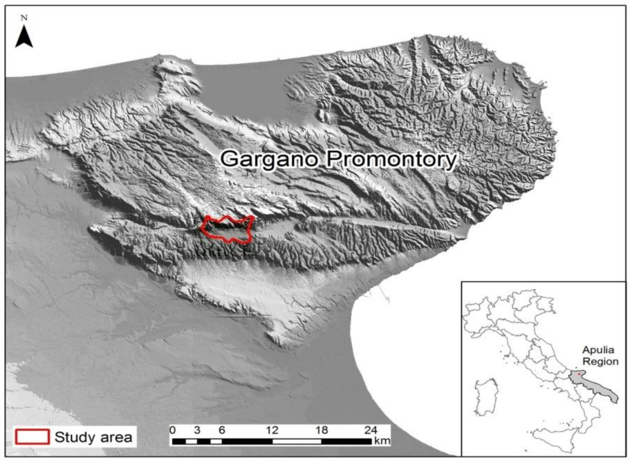
2. The Study Area
3. Materials and Methods
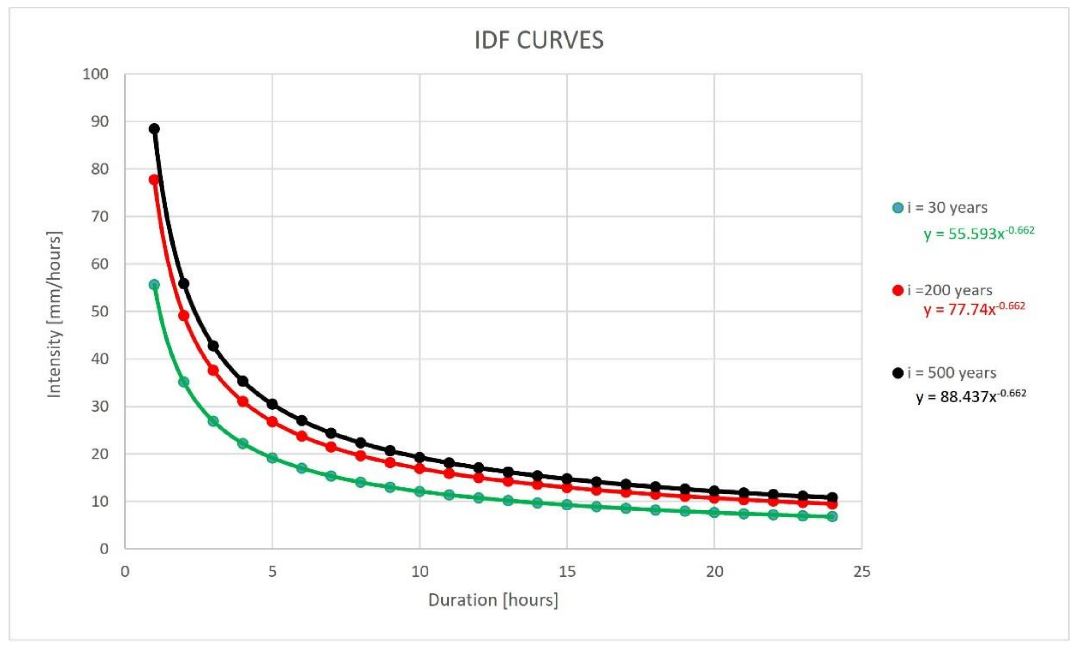
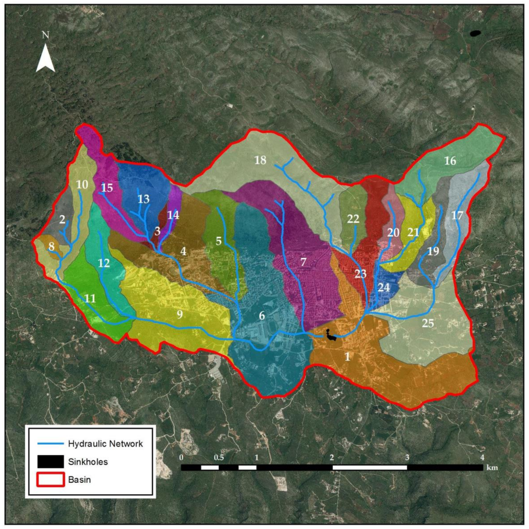
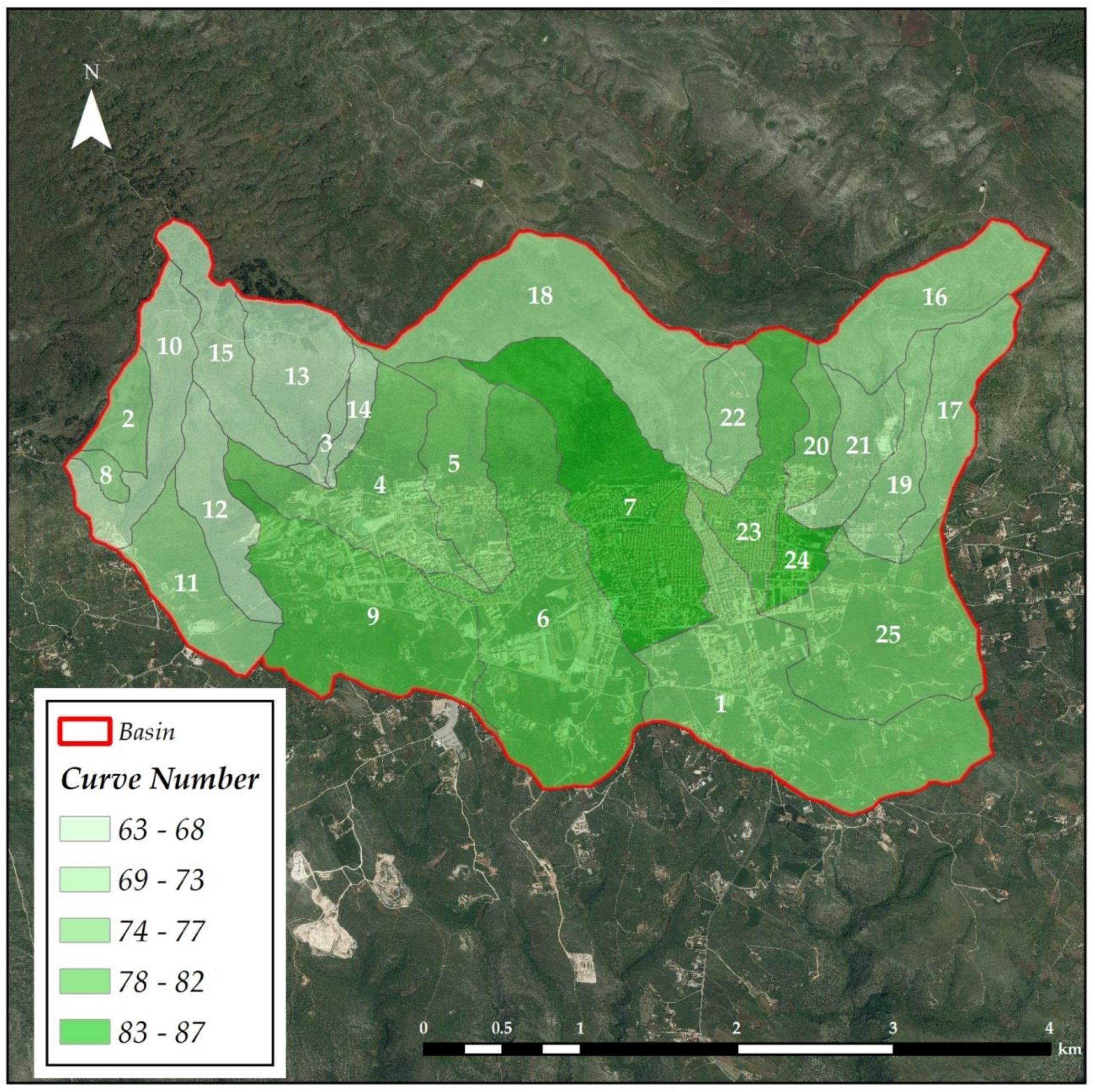
3.1. Hydrologic Modeling
- im is the average intensity of rain, a function of the duration of the rainfall event (t) and of the return period (TR);
- a is a parameter depending on the return period (TR);
- n is a parameter that defines the decrease of rainfall intensity over time.
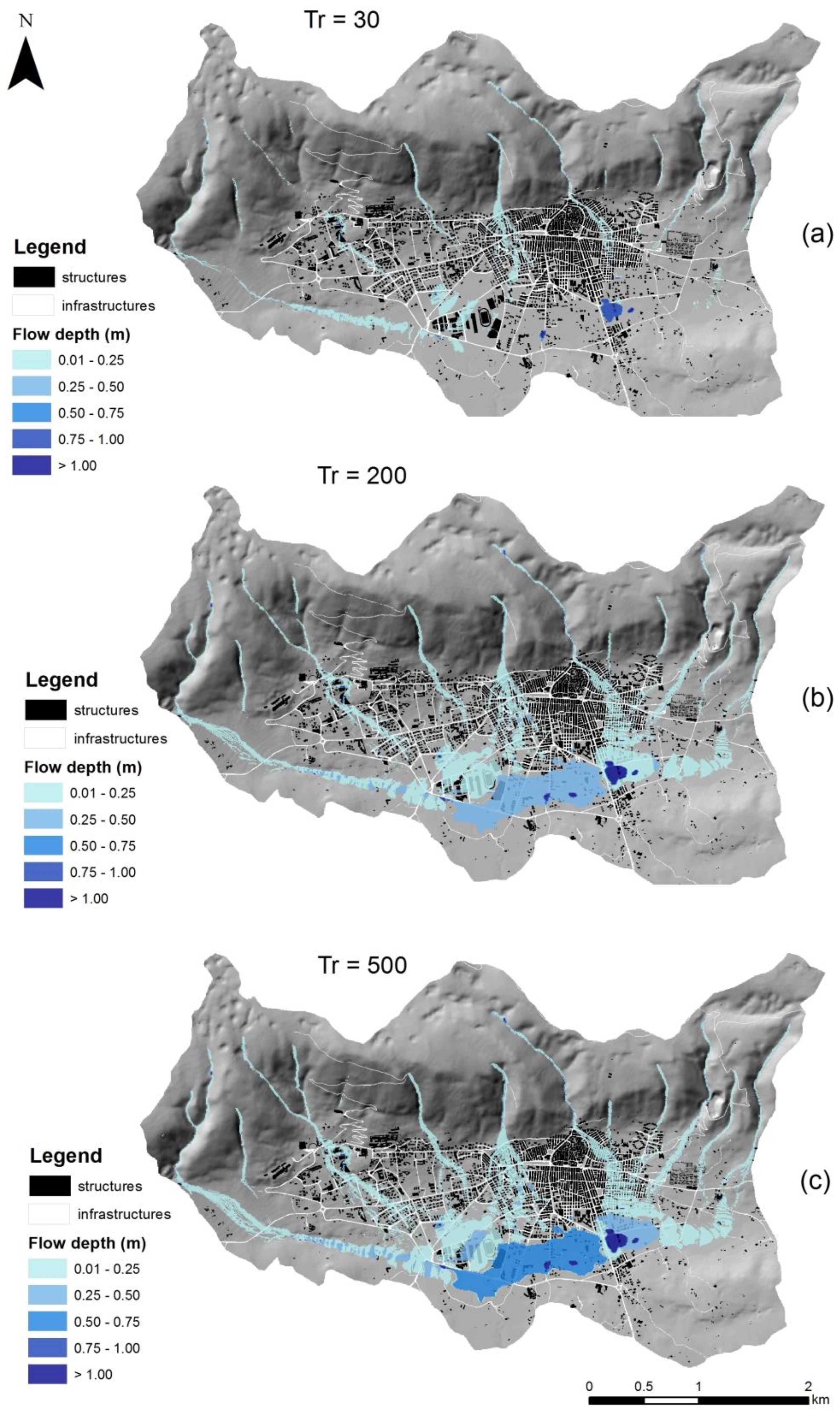
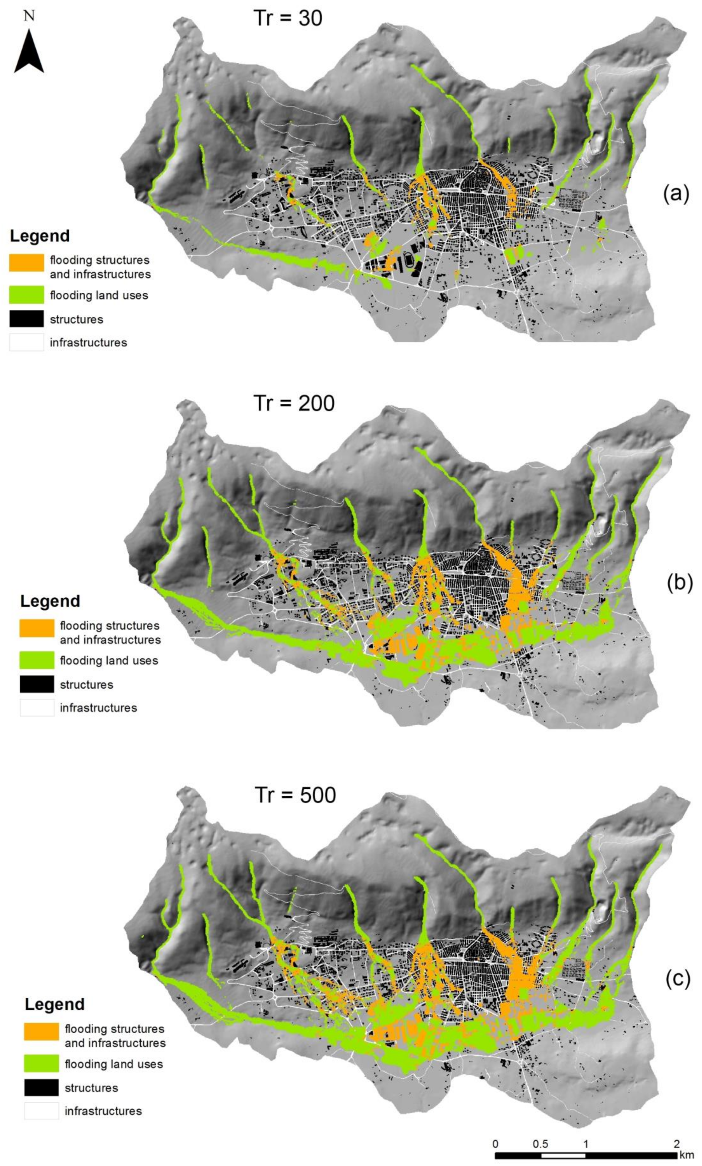
- Scenario 1: TR = 30 years;
- Scenario 2: TR = 200 years;
- Scenario 3: TR = 500 years.
- h represents the height of rainfall (expressed in millimeters of precipitation);
- z is the mean elevation of the basin. In this case it is about 684 m.
- ARF is the ratio of the mean areal rainfall (hs) to the mean point rainfall (hp) in the same area. It is a function of time (t), basin area (A), and return period (TR);
- hs is the mean areal rainfall and is a function of time (t), basin area (A), and return period (TR);
- hp is the mean point rainfall and is a function of time (t) and return period (TR).
3.2. Hydraulic Modeling
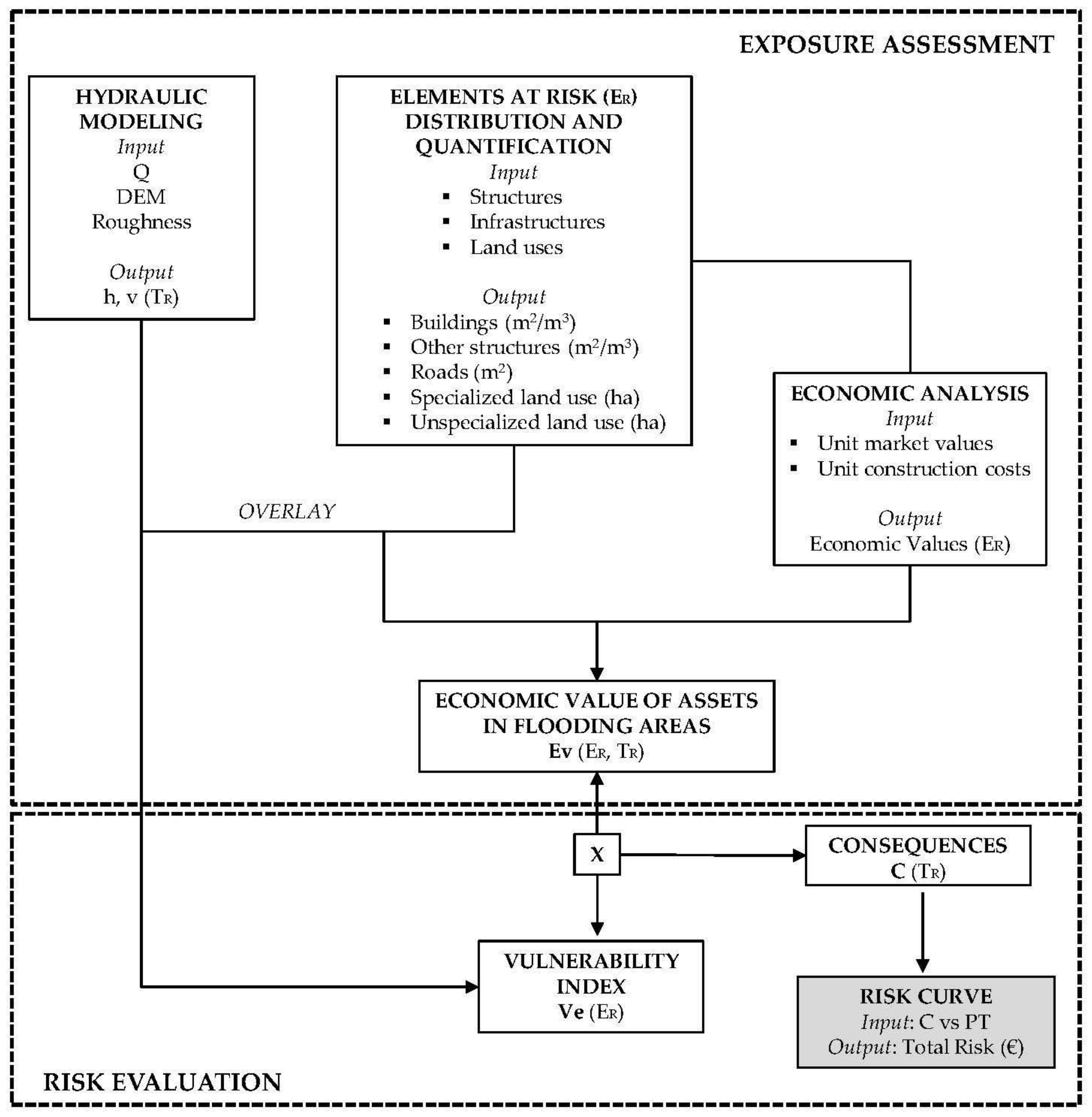
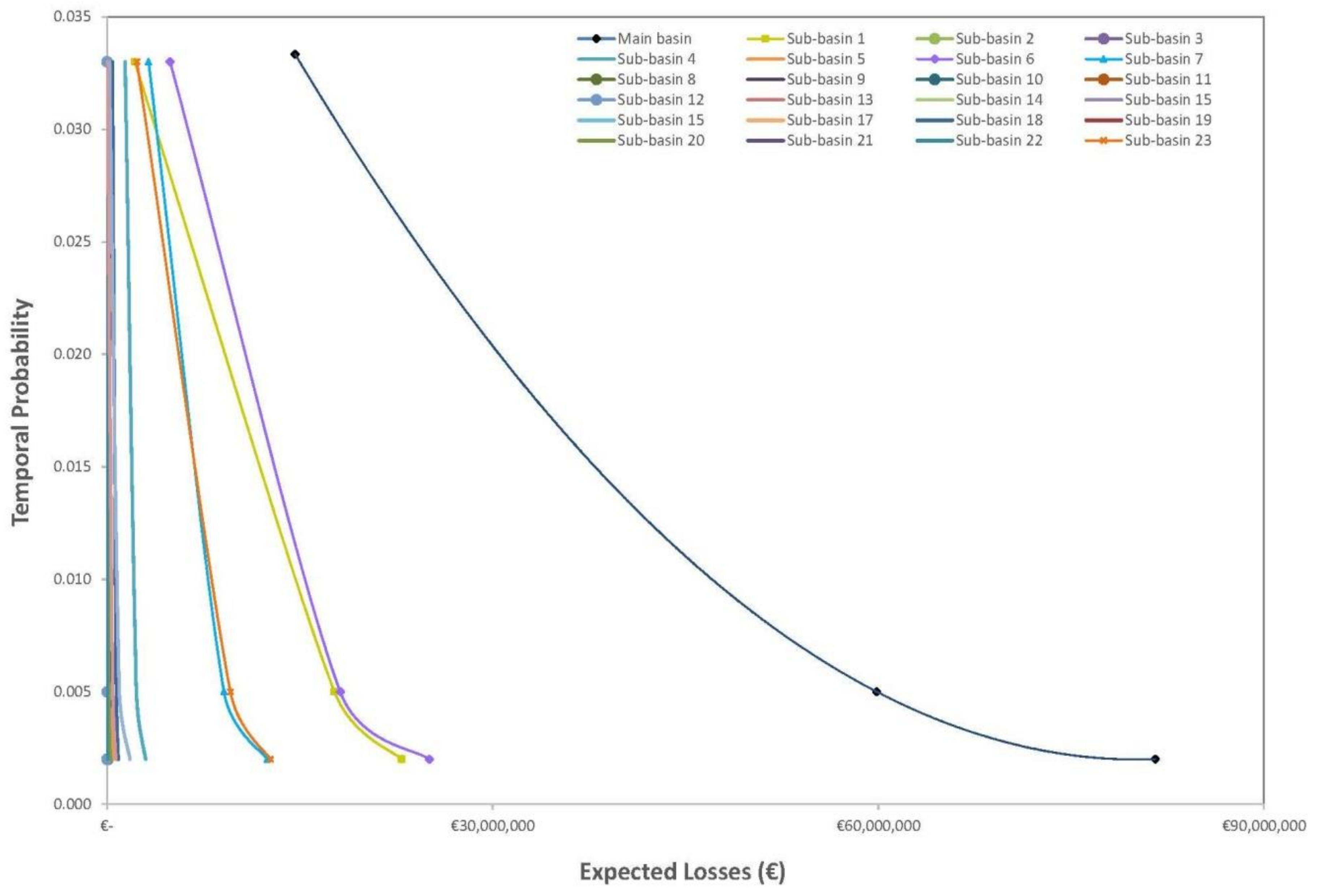
3.3. Risk Assessment
4. Results and Discussion
5. Conclusions
Acknowledgments
Author Contributions
Conflicts of Interest
References
- United Nations International Strategy for Disaster Reduction Secretariat. Global Assessment Report on Disaster Risk Reduction; United Nations International Strategy for Disaster Reduction Secretariat: Geneva, Switzerland, 2009; pp. 1–207. ISBN 9789211320282. [Google Scholar]
- Carrera, L.; Standardi, G.; Bosello, F.; Mysiak, J. Assessing direct and indirect economic impacts of a flood event through the integration of spatial and computable general equilibrium modelling. Environ. Modell. Softw. 2015, 63, 109–122. [Google Scholar] [CrossRef]
- Apollonio, C.; Balacco, G.; Novelli, A.; Tarantino, E.; Piccinni, A.F. Land Use Change Impact on Flooding Areas: The Case Study of Cervaro Basin (Italy). Sustainability 2016, 8, 996. [Google Scholar] [CrossRef]
- Novelli, A.; Tarantino, E.; Caradonna, G.; Apollonio, C.; Balacco, G.; Piccinni, F. Improving the ANN Classification Accuracy of Landsat Data Through Spectral Indices and Linear Transformations (PCA and TCT) Aimed at LU/LC Monitoring of a River Basin. In Proceedings of the 16th International Conference on Computational Science and Its Applications, Beijing, China, 4–7 July 2016; Gervasi, O., Murgante, B., Misra, S., Rocha, A.M.A.C., Torre, C.M., Taniar, D., Apduhan, B.O., Stankova, E., Wang, S., Eds.; Springer: Beijing, China, 2016; pp. 420–432. [Google Scholar]
- European Environmental Agency. Economic Losses from Climate-Related Extremes. European Environmental Agency, 2017. Available online: https://www.eea.europa.eu/data-and-maps/indicators/direct-losses-from-weather-disasters-3/assessment/#economic-losses-from-climate-related-extremes (accessed on 29 March 2018).
- Glade, T.; Anderson, M.; Crozier, M.J. Landslide Hazard and Risk; John Wiley & Sons, Ltd.: Chichester, UK, 2005; pp. 1–824. ISBN 9780471486633. [Google Scholar]
- Pellicani, R.; Argentiero, I.; Parisi, A.; Fidelibus, M.D.; Spilotro, G. Resilience modification and dynamic risk assessment in hybrid systems. Study cases in underground settlements of Murgia edge (Apulia, Southern Italy). In International Conference on Computational Science and Its Applications; Gervasi, O., Murgante, M., Misra, S., Borruso, G., Torre, C.M., Rocha, A.M., Taniar, D., Apduhan, B.O., Stankova, E., Cuzzocrea, A., Eds.; Springer: Cham, Switzerland, 2017; Volume 10405, pp. 230–245. ISBN 978-3-319-62394-8. [Google Scholar]
- Armenakis, C.; Nirupama, N. Estimating spatial disaster risk in urban environments. Geomat. Nat. Hazards Risk 2013, 4, 289–298. [Google Scholar] [CrossRef]
- Merz, B.; Kreibich, H.; Schwarze, R.; Thieken, A. Assessment of economic flood damage. Nat. Hazards Earth Syst. Sci. 2010, 10, 1697–1724. [Google Scholar] [CrossRef]
- Dutta, D.; Herath, S.; Musiake, K. Direct Flood Damage Modeling Towards Urban Flood Risk Management; International Center for Urban Safety Engineering: Tokyo, Japan, 2001; pp. 127–143. [Google Scholar]
- Mekong River Commission Secretariat. Best Practise Guidelines for Flood Risk Assessment. The Flood Management and Mitigation Programme Component 2: Structural Measures & Flood Proofing in the Lower Mekong Basin. 2009. Available online: http://www.preventionweb.net/files/15958_mrcbestpractiseguidelinesforfloodri.pdf (accessed on 29 March 2018).
- Nones, M.; Pescaroli, G. Implications of cascading effects for the EU Floods Directive. Int. J. River Basin Manag. 2016, 14, 195–204. [Google Scholar] [CrossRef]
- Pescaroli, G.; Alexander, D. A definition of cascading disaster and cascading effects: Going beyond the ‘topping dominoes’ metaphor. Planet@Risk 2015, 3, 58–67. [Google Scholar]
- Pellicani, R.; Van Westen, C.J.; Spilotro, G. Assessing landslide exposure in areas with limited landslide information. Landslides 2014, 11, 463–480. [Google Scholar] [CrossRef]
- Barbano, A.; Braca, G.; Bussettini, M.; Dessì, B.; Inghilesi, R.; Lastoria, B.; Monacelli, G.; Morucci, S.; Piva, F.; Sinapi, L.; et al. Proposta metodologica per l’aggiornamento delle Mappe di Pericolosità e di Rischio—Attuazione della Direttiva 2007/60/CE Relativa alla Valutazione e alla Gestione dei Rischi da Alluvioni (Decreto Legislativo n.49/2010); ISPRA: Rome, Italy, 2012. Available online: http://www.isprambiente.gov.it/files/pubblicazioni/manuali-lineeguida/MLG_82_2012.pdf (accessed on 29 March 2018).
- Huizinga, J.; de Moel, H.; Szewczyk, W. Global flood depth-damage functions—Methodology and the database with guidelines. Joint Res. Center 2017. [Google Scholar] [CrossRef]
- Van Westen, C.J.; Luna, B.Q.; Franco, R.V. Development of training materials on the use of geo-information for multi-hazard risk assessment in a mountainous environment. In Proceedings of the Mountain Risks International Conference, Firenze, Italy, 24–26 November 2010; Malet, J.-P., Glade, T., Casagli, N., Eds.; CERG: Strasbourg, France, 2010; pp. 469–475. [Google Scholar]
- Flood Directive 2007/60/EC of the European Parliament and of the Council of 23 October 2007 on the Assessment and Management of Flood Risks. Available online: http://eur-lex.europa.eu/legal-content/EN/TXT/?uri=CELEX:32007L0060 (accessed on 29 March 2018).
- Martinotti, M.E.; Pisano, L.; Marchesini, I.; Rossi, M.; Peruccacci, S.; Brunetti, M.T.; Melillo, M.; Amoruso, G.; Loiacono, P.; Vennari, C.; et al. Landslides, floods and sinkholes in a karst environment: The 1–6 September 2014 Gargano event, southern Italy. Nat. Hazards Earth Syst. Sci. 2017, 17, 467–480. [Google Scholar] [CrossRef]
- Billi, A.; Salvini, F. Sistemi di fratture associati a faglie in rocce carbonatiche: Nuovi dati sull’evoluzione tettonica del Promontorio del Gargano. Boll. Soc. Geol. Ital. 2000, 119, 237–250. [Google Scholar]
- Patacca, E.; Scandone, P. Geology of the Southern Apennines. Ital. J. Geosci. 2007, 7, 75–119. [Google Scholar]
- Sezione di Protezione Civile—Regione Puglia, Annali Idrologici. Available online: http://www.protezionecivile.puglia.it (accessed on 29 March 2018).
- Pellicani, R.; Spilotro, G. Evaluating the quality of landslide inventory maps: Comparison between archive and surveyed inventories for Daunia region (Apulia, Southern Italy). Bull. Eng. Geol. Environ. 2015, 74, 357–367. [Google Scholar] [CrossRef]
- Spilotro, G.; Gallicchio, S.; Pellicani, R.; Diprizio, G. A basic geothematic map for land planning and modeling (Daunian Subapennine—Apulia Region, Italy). In Proceedings of the Computational Science and Its Applications—16th International Conference, Beijing, China, 4–7 July 2016; Springer International Publishing: Cham, Switzerland, 2016; Volume 9788, pp. 107–119. [Google Scholar]
- Rossi, F.; Fiorentino, M.; Versace, P. Two-Component Extreme Value Distribution for Flood Frequency Analysis. Water Resour. Res. 1984, 20, 847–856. [Google Scholar] [CrossRef]
- Fiorentino, V.; Gabriele, S.; Rossi, F.; Versace, P. Hierarchical approach for regional flood frequency analysis. In Regional Flood Frequency Analysis; Singh, V.P., Ed.; D. Reidel: Norwell, MA, USA, 1987; pp. 35–49. [Google Scholar]
- Copertino, V.A.; Fiorentino, M. Valutazione Delle Piene in Puglia; Tipolitografia La Modernissima: Lamezia Terme, Italy, 1994. [Google Scholar]
- Autorità di Bacino della Puglia, Piano Stralcio di Assetto Idrogeologico (PAI). Available online: http://www.adb.puglia.it (accessed on 29 March 2018).
- U.S. Weather Bureau. Rainfall intensity-frequency regime—Part 1: The Ohio Valley. In Technical Paper No. 29 (TP-29); U.S. Weather Bureau: Washington, DC, USA, 1957. [Google Scholar]
- U.S. Weather Bureau. Rainfall intensity-frequency regime—Part 2: The Southeastern United States. In Technical Paper No. 29 (TP-29); U.S. Weather Bureau: Washington, DC, USA, 1958. [Google Scholar]
- U.S. Weather Bureau. Rainfall intensity-frequency regime—Part 3: The Middle Atlantic Region. In Technical Paper No. 29 (TP-29); U.S. Weather Bureau: Washington, DC, USA, 1958. [Google Scholar]
- U.S. Weather Bureau. Rainfall intensity-frequency regime—Part 4: The Northeastern United States. In Technical Paper No. 29 (TP-29); U.S. Weather Bureau: Washington, DC, USA, 1959. [Google Scholar]
- U.S. Weather Bureau. Rainfall intensity-frequency regime—Part 5: The Great Lakes Region. In Technical Paper No. 29 (TP-29); U.S. Weather Bureau: Washington, DC, USA, 1960. [Google Scholar]
- U.S. Weather Bureau. Two- to ten-day precipitation for return periods of 2 to 100 years in the contiguous United States. In Technical Paper No 49 (TP-49); U.S. Weather Bureau: Washington, DC, USA, 1964. [Google Scholar]
- Penta, A. Distribuzione di probabilità del massimo annuale dell’altezza di pioggia giornaliera su un bacino. In Proceedings of the Atti XIV Convegno di Idraulica e Costruzioni Idrauliche, Napoli, Italy, 10–12 October 1974. [Google Scholar]
- Eagleson, P.S. Dynamics of flood frequency. Water Resour. Res. 1972, 8, 878–898. [Google Scholar] [CrossRef]
- NRCS. National Engineering Handbook: Part 630—Hydrology Natural Resources Conservation Service; NRCS: Washington, DC, USA, 2004.
- Deshmukh, D.S.; Chaube, U.C.; Hailu, A.E.; Gudeta, D.A.; Kassa, M.T. Estimation and comparison of curve numbers based on dynamic land use land cover change, observed rainfall-runoff data and land slope. J. Hydrol. 2013, 492, 89–101. [Google Scholar] [CrossRef]
- Kowalik, T.; Walega, A. Estimation of CN parameter for small agricultural watersheds using asymptotic functions. Water 2015, 7, 939–955. [Google Scholar] [CrossRef]
- Mishra, S.K.; Singh, V. Soil Conservation Service Curve Number (SCS-CN) Methodology; Kluwer Academic Publishers: Dordrecht, The Netherlands, 2013; p. 42. [Google Scholar]
- O’Brien, J. FLO-2D Users Manual; FLO-2D Inc.: Nutrioso, AR, USA, 2001. [Google Scholar]
- Lee, E.M.; Jones, D.K.C. Landslide Risk Assessment; Thomas Telford Publishing: London, UK, 2014; p. 454. ISBN 0-7277-3171-8. [Google Scholar]
- Van Westen, C.J.; Van Asch, T.W.J.; Soeters, R. Landslide hazard and risk zonation—Why is it still so difficult? Bull. Eng. Geol. Environ. 2006, 65, 167–184. [Google Scholar] [CrossRef]
- SIT Puglia, Cartografia Tematica. Available online: http://www.sit.puglia.it/portal/portale_cartografie_tecniche_tematiche/home (accessed on 29 March 2018).
- Distretto Idrografico dell’Appennino Meridionale. Autorità di Bacino della Puglia. Available online: http://www.adb.puglia.it/public/page.php?96 (accessed on 29 March 2018).


| Scenario | a | n |
|---|---|---|
| TR 30 | 55.59 | 0.388 |
| TR 200 | 77.74 | 0.388 |
| TR 500 | 88.44 | 0.388 |
| Sub-Basin | Q 30 Years | Q 200 Years | Q 500 Years |
|---|---|---|---|
| (m3/s) | (m3/s) | (m3/s) | |
| 1 | 3.86 | 7.85 | 10.02 |
| 2 | 0.24 | 0.64 | 0.88 |
| 3 | 0.04 | 0.14 | 0.21 |
| 4 | 2.22 | 4.57 | 5.86 |
| 5 | 1.47 | 3.01 | 3.85 |
| 6 | 5.26 | 9.82 | 12.22 |
| 7 | 5.23 | 9.45 | 11.65 |
| 8 | 0.08 | 0.25 | 0.36 |
| 9 | 3.47 | 6.62 | 8.30 |
| 10 | 0.60 | 1.50 | 2.03 |
| 11 | 0.66 | 1.56 | 2.07 |
| 12 | 0.46 | 1.14 | 1.54 |
| 13 | 0.35 | 1.13 | 1.62 |
| 14 | 0.12 | 0.34 | 0.46 |
| 15 | 0.34 | 1.01 | 1.45 |
| 16 | 0.88 | 2.09 | 2.78 |
| 17 | 0.75 | 1.77 | 2.36 |
| 18 | 2.03 | 4.59 | 6.04 |
| 19 | 0.65 | 1.43 | 1.87 |
| 20 | 0.52 | 1.15 | 1.50 |
| 21 | 0.63 | 1.48 | 1.97 |
| 22 | 0.45 | 1.09 | 1.46 |
| 23 | 2.19 | 4.14 | 5.17 |
| 24 | 1.15 | 2.02 | 2.47 |
| 25 | 2.12 | 4.55 | 5.90 |
| Categories of Elements at Risk | Vulnerability (Ve) | Reference | ||
|---|---|---|---|---|
| h (m); v (m/s) | ||||
| Buildings | Ve(h) = 0.5∙h | [15] | ||
| Other structures | Ve(h,v) = | 0.5∙h | if v < 2 | |
| 0.35∙h∙(1 + 0.25∙v) | if v ≥ 2 | |||
| Specialized land use | Ve(h,v) = | h | if v < 0.25 | |
| h∙(1 + v) | if v ≥ 0.25 | |||
| Unspecialized land use | Ve(h,v) = | 0.25∙h | if v < 0.25 | |
| 0.25∙h∙(1 + v) | if v ≥ 0.25 | |||
| Infrastructures | Ve = f(h) | [16] | ||
| Elements at Risk | TR | Temporal Probability | Amount | Economic Value | Consequences | Total Economic Losses |
|---|---|---|---|---|---|---|
| Buildings | 30 | 0.033 | 55,894 mq | €194,614,708 | €13,895,661 | €14,880,090 |
| Other structures | 30 | 0.033 | 7185 mq | €6,109,602 | €694,699 | |
| Road | 30 | 0.033 | 32,020 mq | €4,002,468 | €273,812 | |
| Specialized land use | 30 | 0.033 | 4 ha | €56,527 | €9701 | |
| Unspecialized land use | 30 | 0.033 | 30 ha | €82,544 | €6218 | |
| Buildings | 200 | 0.005 | 187,626 mq | €588,434,156 | €57,397,781 | €59,982,082 |
| Other structures | 200 | 0.005 | 40,472 mq | €10,577,381 | €1,251,951 | |
| Road | 200 | 0.005 | 108,672 mq | €13,584,055 | €1,239,335 | |
| Specialized land use | 200 | 0.005 | 19 ha | €265,619 | €68,215 | |
| Unspecialized land use | 200 | 0.005 | 77 ha | €293,026 | €24,801 | |
| Buildings | 500 | 0.002 | 228,538 mq | €717,485,846 | €77,739,884 | €81,326,517 |
| Other structures | 500 | 0.002 | 47,304 mq | €13,905,091 | €1,744,504 | |
| Road | 500 | 0.002 | 137,329 mq | €17,166,171 | €1,711,906 | |
| Specialized land use | 500 | 0.002 | 22 ha | €304,865 | €94,850 | |
| Unspecialized land use | 500 | 0.002 | 89 ha | €332,429 | €35,373 |
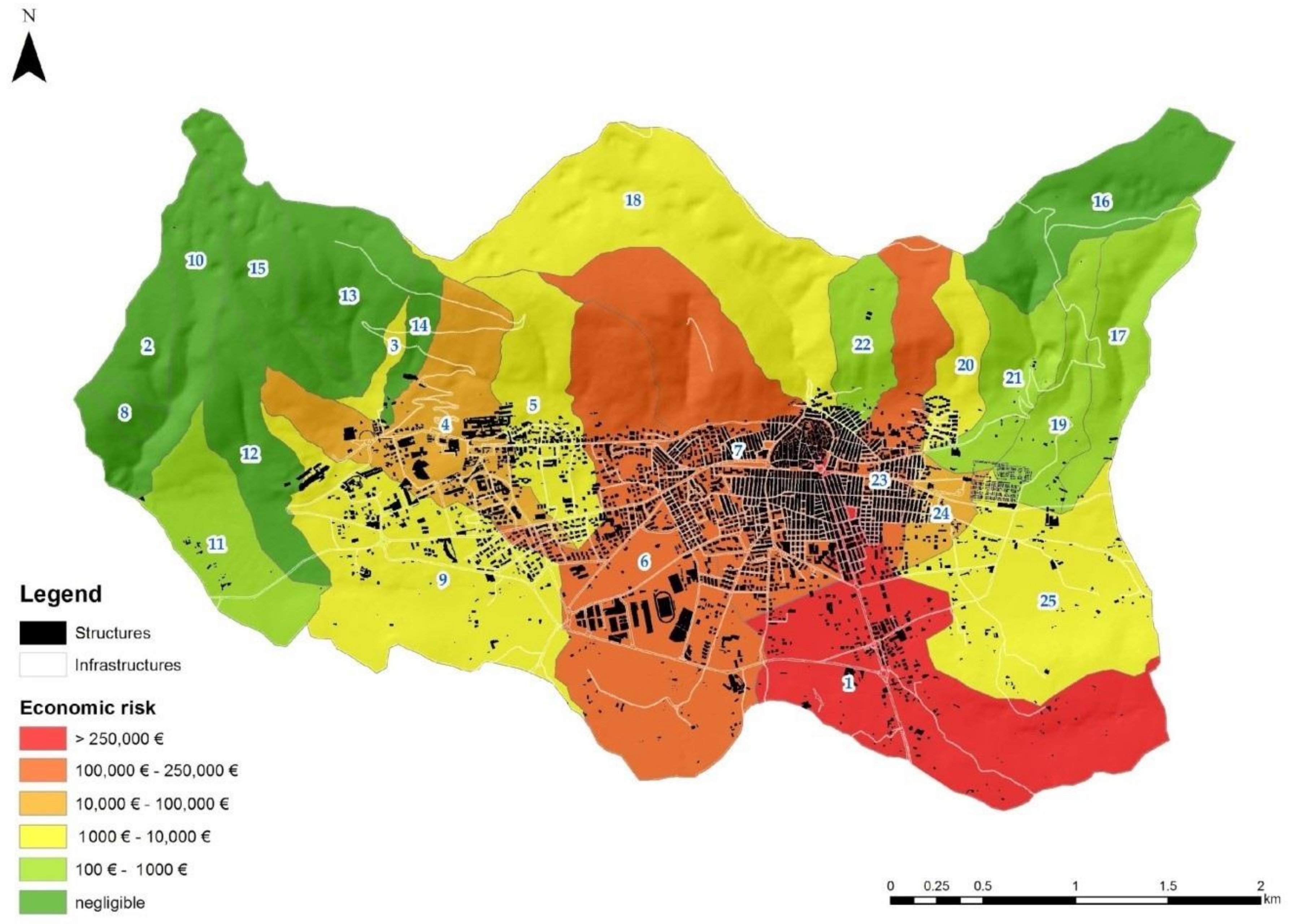
| Sub-Basins | Total Risk | Sub-Basins | Total Risk |
|---|---|---|---|
| 1 | €271,984 | 14 | € ≈ 0 |
| 2 | € ≈ 0 | 15 | € ≈ 0 |
| 3 | €1036 | 16 | € ≈ 0 |
| 4 | €16,031 | 17 | €180 |
| 5 | €3412 | 18 | €5531 |
| 6 | €235,335 | 19 | €343 |
| 7 | €104,698 | 20 | €2610 |
| 8 | € ≈ 0 | 21 | €195 |
| 9 | €6513 | 22 | €430 |
| 10 | €52 | 23 | €128,223 |
| 11 | €146 | 24 | €14,223 |
| 12 | €11 | 25 | €7792 |
| 13 | €2.6 |
© 2018 by the authors. Licensee MDPI, Basel, Switzerland. This article is an open access article distributed under the terms and conditions of the Creative Commons Attribution (CC BY) license (http://creativecommons.org/licenses/by/4.0/).
Share and Cite
Pellicani, R.; Parisi, A.; Iemmolo, G.; Apollonio, C. Economic Risk Evaluation in Urban Flooding and Instability-Prone Areas: The Case Study of San Giovanni Rotondo (Southern Italy). Geosciences 2018, 8, 112. https://doi.org/10.3390/geosciences8040112
Pellicani R, Parisi A, Iemmolo G, Apollonio C. Economic Risk Evaluation in Urban Flooding and Instability-Prone Areas: The Case Study of San Giovanni Rotondo (Southern Italy). Geosciences. 2018; 8(4):112. https://doi.org/10.3390/geosciences8040112
Chicago/Turabian StylePellicani, Roberta, Alessandro Parisi, Gabriele Iemmolo, and Ciro Apollonio. 2018. "Economic Risk Evaluation in Urban Flooding and Instability-Prone Areas: The Case Study of San Giovanni Rotondo (Southern Italy)" Geosciences 8, no. 4: 112. https://doi.org/10.3390/geosciences8040112