Drought Prediction System for Central Europe and Its Validation

Abstract

In recent years, two drought monitoring systems have been developed in the Czech Republic based on the SoilClim and AVISO soil moisture models. The former is run by Mendel University and Global Change Research Institute (CAS), while the latter, by the Czech Hydrometeorological Institute. SoilClim is based more on real soil properties and aimed primarily at agriculture, while AVISO complements the system with more theoretical presumptions about soil, showing, rather, climatological potential. Both soil moisture models were complemented by forecasts on a daily basis, taking meteorological inputs from NWP (Numerical Weather Prediction) models and thus giving short- to mid-range outlooks up to 9 days ahead. Validation of the soil moisture and drought intensity prediction was performed and is presented in this article showing its prediction reliability and potential. In the analysis, we focus mainly on the past year, 2017. The tool has strong predictive power for soil moisture and drought intensity so it is suitable for farmers who need to make decisions about irrigation and production activities. The presented system is fully functional and can be applied in the coming years.

1. Introduction

Drought forecast is important for various fields of human activity, such as agriculture, hydrology, the energy sector, human health, etc. (e.g., [1,2,3]). There are many existing drought monitoring systems in the world nowadays. An overview of some of these can be found on the National Drought Mitigation Center web pages (http://drought.unl.edu/MonitoringTools/InternationalEarlyWarning.aspx). The focus and target audience of those services may differ to quite an extent, as drought itself is a complex phenomenon. Some of the systems include a forecast component as well. In general, to predict drought conditions, one can either consider statistical or dynamical methods [4]. The former are based on the long-term correlation of global circulation patterns with the regional weather, while the latter utilize the numerical weather prediction (NWP) models and their ensembles. The simplest drought forecast includes information on air temperature and precipitation and their anomalies within the course of several days to months. Meteorological parameters can be further combined into basic drought indices or included in the input of hydrological, agricultural, or other models. The various applications or needs regarding drought forecasting and warming were recently published in a special issue of Hydrology and Earth System Sciences (e.g., [5,6,7]). An overview of principles of the drought prediction over different time scales was discussed by [8]. There are three main components of drought forecasting: a set of input variables, methodologies, and the outputs obtained. The selection of input variables depends on what kind of drought should be forecasted. The input variables may include basic hydro-meteorological parameters, e.g., precipitation, air temperature, evaporation, soil moisture or streamflow, their combination in a form of drought indices, or climate indices related to large-scale atmospheric or oceanic circulation, e.g., El Nino-Southern Oscillation (ENSO). A range of methodologies is very wide and again strongly dependent on whichever drought is to be forecasted. These methods include different statistical approaches, e.g., regression models, time series models, or neural network models. For more details on individual methods we refer to [8]. The last component of the drought forecasting is the final output that may include information on the onset and termination of the drought, its severity, or its probability of occurrence. Many of the contemporary approaches developed for drought forecasting aim to deliver an outlook on longer time scales from weeks to months. When the interest goes to shorter time frames of days and weeks, the weather forecast delivered by NWP models plays a key role in the drought prediction.

The outputs of weather models are always influenced by an uncertainty that grows over time and decreases the forecast accuracy on different spatial scales: earlier on the local scale, later on the global scale. Errors in the NWP forecast stem from several sources that are related to, for instance, the NPW models themselves (settings of model dynamics and physics, numerical methods) or the initial condition at the beginning of each forecast (availability, accuracy, spatial homogeneity of meteorological observations, data assimilation, and interpolation to the model grid). The validation of NWP models is an important step needed to understand the reliability of forecasts based on the NWP model. In general, the validation can be a complex process and includes, for instance, testing the assumptions on which the model is built. However, the most frequently used part of the validation process in meteorology is the comparison of model outputs with real observations. There are many datasets of weather observations against which the NWP models and forecasts can be tested. These include the ground weather stations, upper air soundings, satellite observations, and many others, often combining data from more independent sources, like re-analysis. In this study, we validate the forecasts of the NWP model and the skill of the soil model against the station measurements carried out and provided by Czech Hydrometeorological Institute. The validation data and methods are described in the following chapters.

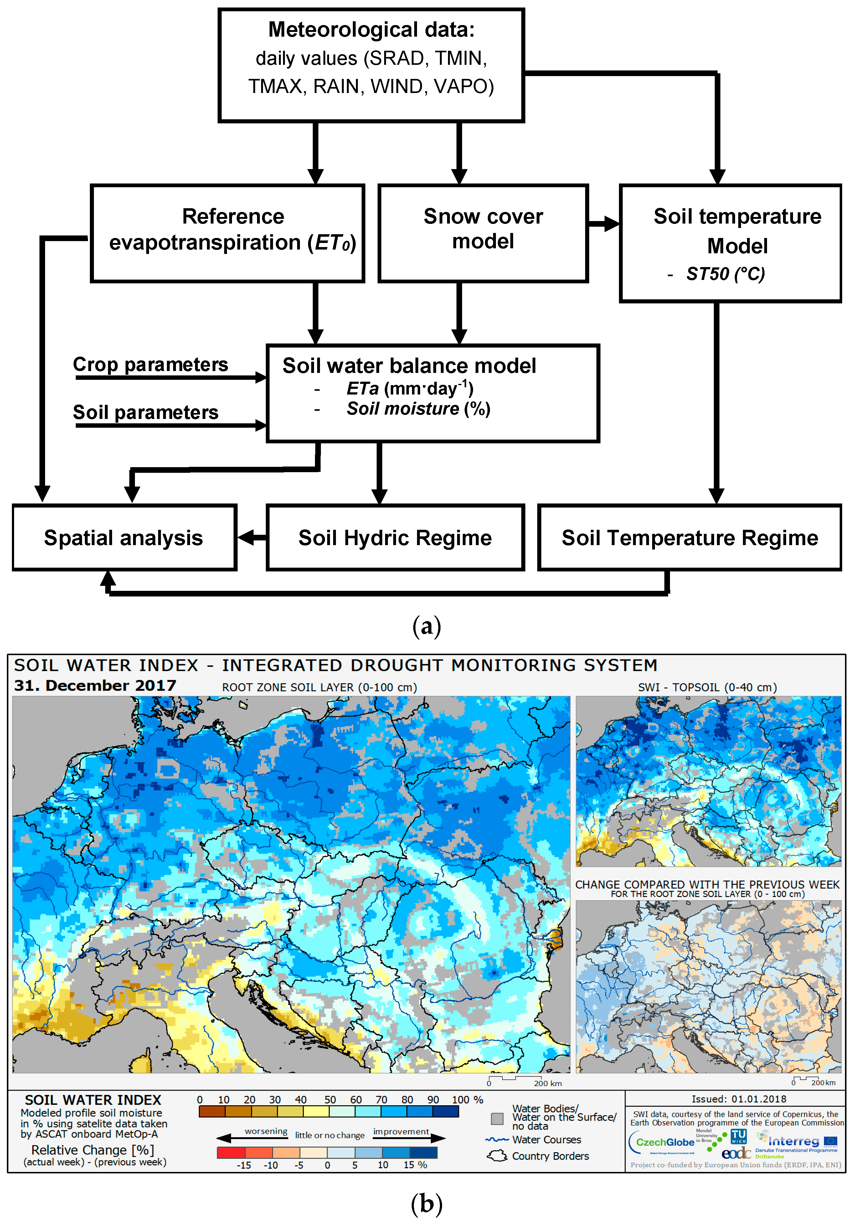
Within the last years, two drought monitoring systems were developed in the Czech Republic in part in collaboration with neighboring countries. These two systems complement each other. The system primarily based on the SoilClim soil moisture model has been developed and is being run by the Global Change Research Institute (GCRI) of CAS (Czech Academy of Sciences), Mendel University, and State Land Office using data support of the Czech Hydrometeorological Institute (CHMI). It has been designed to target agriculture drought, including impacts [9]; besides soil moisture model relies on remote sensing and drought reporting data. Most detailed information at highest resolution covers Czech Republic and Slovakia using SoilClim (Figure 1a) as the primary tool. Due to the use of remote sensing data it is able to provide contextual information on the ongoing drought episode from a much wider area of Central Europe (Figure 1b). The system based on the AVISO soil moisture model, run by the Czech Hydrometeorological Institute (CHMI), is focused on soil and meteorological drought. Both systems work with daily data. The SoilClim weather inputs are interpolated to 500 m grid, and the model differentiates the upper (0–40 cm profile) and lower soil layers (40–100 cm), while AVISO works with one soil layer (1–100 cm) and relies on the station approach. After several years of tuning both models, they are now also being utilized for a soil moisture (drought) forecast for several days ahead. For the SoilClim model, a long-term statistical forecast (8 weeks ahead) based on analogs also exists. In this paper, we deal only with the short to medium range forecasts. Thanks to common activities (national projects, etc.), there are plans for both monitoring systems, initially developed separately, to be presented in one place (a web portal), taking advantage of mutual cooperation and covering meteorological and agricultural drought. The website will provide users with more robust information about various aspects of drought, validation of the predictions, etc.

The aim of the system is, among others, to improve decision-making processes through reliable forecasts, particularly in the agricultural sector, and thus to increase both the economical and ecological effectiveness of agriculture production.

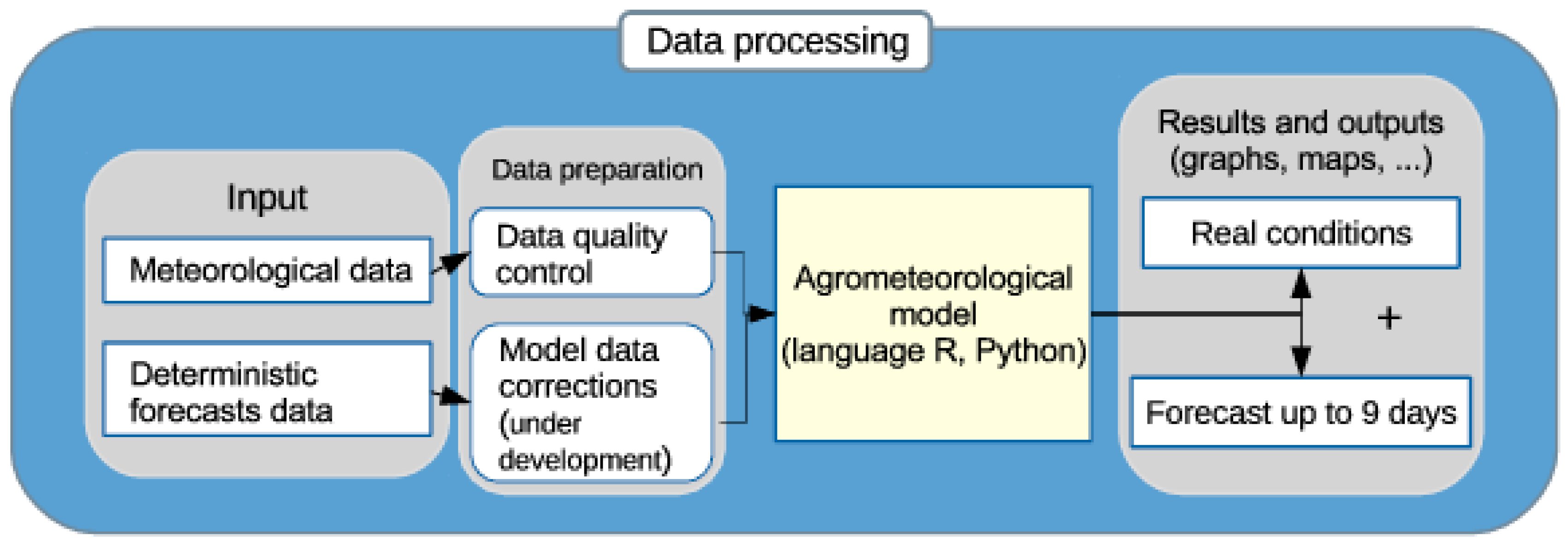
In this article, we present both soil moisture models; we then present the NWP models used as input into these models to retrieve the soil moisture forecast, and in the end, we give the results of the validation of the outputs (drought characteristics forecast) of both systems.

2. Materials and Methods

2.1. SoilClim

The SoilClim model (Figure 1a) is designed to study root-zone soil moisture content (from the surface down to 1.0 m or less in shallow soils) using the modelling approach suggested by [10], which was partially modified by [11] and validated, e.g., by Ref. [12]. Only the soil moisture available to plants (i.e., above wilting point) was considered when soil moisture was expressed in mm or in relative terms. In the latter case, the total volume of water that would be available to plants was calculated as the difference between soil moisture at field capacity and wilting point multiplied by layer’s depth. SoilClim was applied for each grid and accounted not only for the soil water holding capacity but also for the type of vegetation cover, phenology development, root growth, or snow cover accumulation/melting [13]. The module for actual evapotranspiration (ETa) and soil water content estimates considers two soil layers: the topsoil layer (from the ground surface to 0.4 m depth) and the subsoil layer (between 0.4 and 1.0 m). The cascading approach for transferring water from the topsoil to subsoil layers is used when the topsoil is less than 50% saturated. In the case of higher soil water content in the topsoil, proportion of soil water in the topsoil is allowed to seep into the subsoil, mimicking the macropore and preferential water transport. While the model allows one to estimate runoff and interception, the study considered only the latter part, as it did not consider precipitation data correction through wind-speed. The Czech Hydrometeorological Institute, as the official data provider, uses unshielded Hellman-type raingauges and does not carry out the precipitation data correction routinely. The precipitation is likely underestimated by 5–10% on an annual basis (e.g., [14]) and even more in particular events depending on the wind-speed. This was indirectly confirmed when observed soil moisture and SoilClim estimates (not considering run-off) were compared at sites with known actual evapotranspiration, finding no systematic overestimation by SoilClim. SoilClim has dynamically simulated vegetation cover that allows for changing parameters of the canopy (e.g., root depth or crop height) during the growing season based on the thermal time and vernalization requirement (in case of winter crops and perennials). Therefore, the crop parameter Kc [10], as well as root growth dynamics, varies for individual vegetation covers and throughout the year (or vegetation season). The model also accounts for the interception by vegetation depending on the vegetation type and phenological stage, as well as for the soil water percolation below the subsoil layer.

The input climatological data were complemented with values of the maximum soil water holding capacity (MSWC) for both soil layers in each grid cell, which is of critical importance for the dynamic of the actual soil water content. The MSWC for each grid was estimated using a combination of digitalized maps of soil types (1:500,000), detailed soil physics data from 1073 soil pits collected by the Czech National Soil Survey, and data derived from digital maps provided by the Research Institute for Soil and Water Conservation (http://www.vumop.cz/ (accessed on 20 February 2013)) and the European Soil Database [15]. The MSWC was calculated assuming a 1.3 m soil profile unless soil database indicated shallower soil depth. The topsoil (0–0.4 m) and subsoil (0.41–1.0 m or maximum rooting depth when it is shallower) layers had their properties defined separately based on the soil data available. The number of soil layers was limited by the available soil data, which would not allow for meaningful description of more soil layers than top and subsoils. Finally, areas were identified that have at least some part of their growing season influenced by high underground water tables (that are likely to be reached by roots for natural subsurface irrigation) and therefore respond to drought differently (both in terms of the stress magnitude and timing) compared to other rain-fed grid cells. The soils with an observed gleyic process, within close proximity (and at the same altitude) of water bodies and peat and bog areas, were treated differently in the course of soil moisture calculations, and the soil moisture depletion rate was slowed significantly compared to neighboring grids without such influence. This approach (relying on the observed soil properties and detailed elevation and land use models) is, in our opinion, better than using the [16] global dataset, which still requires ground verification in the Czech Republic and also has a coarser spatial resolution. In total, 9.5% of the study area was influenced by high underground water table.

Vegetation cover of the Czech territory was divided into the following categories: (i) arable land (46.2% of the area), (ii) permanent grasslands (7.6%), (iii) conifer forest (20.3%), (iv) deciduous forest (3.1%), (v) mixed forests (6.0%), (vi) other agricultural areas (8.7%), and (vii) grids where no calculation was performed (i.e., urbanized areas (7.0%) and water bodies (1.1%)). The information about the land cover relied on the Corine land cover (CLC2006) 100 m (version 12/2009). Assessment of the annual water balance is made more difficult by the fact that arable land (which dominates the landscape) consists of an ever-changing mixture of crops. In these grids, we considered a 5:4:1 mixture of spring and winter C3 crops (based on present spring barley and winter wheat cultivars) and spring C4 crops (maize)—i.e., calculations on these grids were performed for all three crop types and then a weighted mean was used. The 5:4:1 ratio is based on the mean cultivation area of each crop group between 1961 and 2012. Soil moisture dynamics were then determined as the weighted mean of moisture estimates under all three covers within the given season and grid and have been used also in Ref. [17] or Ref. [18].

The SoilClim model showed very good ability to replicate seasonal dynamics of soil moisture, as well as actual evapotranspiration and long-term trends [12]. The SoilClim model was able to reproduce actual daily evapotranspiration (ETa), explaining between 74% and 80% of the variability. SoilClim also performed well at the lysimetric station Hirschstetten in Austria (in the period 1999–2004) for all three soils, explaining up to 63% (topsoil) and 74% (subsoil) of observed soil moisture variability. Even better results were reported for the Domanínek station (2 seasons under grass cover), in which the SoilClim model explained 63% of topsoil and 74% subsoil soil moisture variability. Ref. [12] showed that SoilClim estimates reproduce fairly well changes in the long-term soil moisture dynamics in the topsoil for the AMJ and JAS periods. In both considered periods, the model underestimated the soil moisture trend on 3 sites and overestimated it also on 3 sites.

2.2. AVISO

Primarily, the AVISO model was designed to analyze soil water content with regard to the influence of climate conditions and the actual course of meteorological elements. Due to the purpose of its utilization at CHMI and also with regard to the need for a uniform comparison of the areas within the Czech Republic with the dominant consideration being the influence of climate conditions, the modeling process and the outputs used are subject to a certain degree of simplification and generalization. This allows comparison of the impacts of changing weather conditions during the season in the different regions in terms of soil water content. It also helps with complication due to the fact that the soil conditions in the Czech Republic are very varied, even in the wider neighborhood of climatological stations where the meteorological elements are measured.

The Czech Hydrometeorological Institute currently conducts the monitoring of meteorological and agricultural drought using its own agrometeorological model, AVISO. The characteristics of evapotranspiration, basic water balance, and soil water content are modeled and analyzed in general to establish the influence of weather processes and climate conditions on the state and development of drought.

The AVISO agrometeorological model is based on the English model MORECS (“The Meteorological Office Rainfall and Evaporation Calculation System“), version I. and II. [19,20,21,22,23]. Currently, the core of the model, with computational algorithms, was reprogrammed into the R language environment. The additional modules for the preparation of various data inputs, spatial calculation, creation of maps, and also input forecast data processing are made in Python.

The main output is the calculation of evapotranspiration, which is then combined with an amount of precipitation data, information about soil conditions, and phenological data for estimation of soil water content. The AVISO agrometeorological model is applied globally for the whole area of the Czech Republic, with the outputs produced in daily steps and primarily for the grasslands. Nevertheless, the information for other agricultural crops and types of land covers are processed too [10].

For the evaluation of loss of water from the upper soil profile by evapotranspiration, the modified (for the specific conditions of the Czech Republic) Penman-Monteith equation, with the temperature of evaporating surface correction and an evaluation of air humidity by means of vapor pressure, was applied [24]. The calculation of evapotranspiration is processed separately for the day and night parts of the day and the resulting value is given by their sum. The daily values of air temperature, water vapor pressure, wind speed, precipitation total, and sunshine duration served as inputs to the model. For actual soil water condition expression, the specific moisture characteristics (hydrolimits as available water capacity, field moisture capacity, wilting point) for the analyzed locality are necessary. In accordance with soil condition simplification and uniformity for the most common soil types throughout the Czech Republic, three groups of soil types (by clay particles) [25] are used:

-

light soil (sandy to loamy-sandy, c.p. 0–20%), AWC (available water capacity) = 70 mm/1 m

-

heavy soil (clayey-loamy to clayey, c.p. 45–75%), AWC = 120 mm/1 m

-

medium-heavy soil (sandy-loamy to loamy, c.p. 20–45%), AWC = 170 mm/1 m

In the case of the calculation of the soil water content in the AVISO model [26], a simplified two-layer model of water movement in the soil with its constant drainage in the whole active profile, which means the soil profile to the depth of active sprouting is used.

As one of the results, the actual soil water deficit is computed as a sum of the difference between precipitation and evapotranspiration of the actual day and soil water deficit at the end of the last day. The soil water content in percent of available water capacity is then calculated by means of the actual soil water deficit value between of two main hydrolimits: field moisture capacity and wilting point (Figure 2).

At present, this model is also experimentally used to process data from the numerical weather forecast (Figure 3) in order to predict future development of soil moisture content and the potential occurrence and intensity of drought. The source data of the deterministic forecast comes from the numerical forecast model, IFS-ECMWF. The possible uses and reliability of the forecast are analyzed by comparing them with datasets from the previous seasons. This includes an analysis of the differences between agrometeorological characteristics derived from measured and modeled data and the differences are also assessed for particular locations.

2.3. NWP Models

Numerical weather prediction models are the backbone of contemporary weather forecasting. They offer time series of a wide range of meteorological quantities, covering the period and (geographical) area of interest. These time series are usually available on a rectangular grid at the surface and also on the vertical levels of the atmosphere. While the computational time step of numerical models is generally few minutes, the results are offered in longer intervals: usually in one- or three-hour steps.

Our project utilizes global versions of numerical weather prediction models and a deterministic setup of their forecasts (in contrast to the ensemble setup also produced by the models). A deterministic setup offers significantly higher resolution compared to ensemble forecasts, which are the preferable choice for the relatively small area of the Czech Republic. Global models are our choice due to the longer forecasted periods compared to regional/limited area models, whose forecasts are usually available only up to 2–3 days. In

Table 1. Summary of the global forecast models and parameters of the forecast outputs.

Forecast Producer	Model	Horizontal Resolution (km)	Frequency of Outputs (h)	Forecast Length (d)
ECMWF	Integrated Forecast System (IFS)	12	3	7
Météo France	ARPÉGE	10	1	4
UK Met Office	Unified Model Global (GUM)	16	1	6
NOAA NCEP	Global Forecasting System (GFS)	25	3	14
Canadian Meteorological Centre	Global Earth Model (CMC)	25	3	6

below, all five utilized models are lined up in descending order. The uppermost model has the highest weight, while the lowermost model has the smallest weight when averaging their results (using the weighted average method for individual forecasted quantities). The table also contains information on meteorological centers operating individual models, frequency of model output, spatial resolution, and forecast length.

There are also other global models available being operated by German, Brazilian, or Japanese meteorological services, as examples. Their outputs, however, are not available in sufficient temporal or spatial resolution or do not perform sufficiently for our region.

3. Results

The SoilClim system gives information in 500 m resolution grids, while AVISO currently gives its outputs for station locations (reflecting the measurement network of CHMI). For general comparison (which is also used on the webpage of www.drought.cz), the results are shown for the whole Czech Republic. In the case of SoilClim, we use aggregated values (averages) over all grids in the Czech Republic, while in the case of AVISO, we used an average over all stations (198 automatic stations) in the system.

In the case of SoiClim, the NWP outputs are bias corrected (by means of the DAP method based on quantile mapping, [27,28]), applied on daily values, taking station measurements as reference series, and, at the same time, the NPW model grid points are localized into station locations. From such station-located series, maps for each meteorological element are created, which serve as input into the SoilClim model. Interpolation is performed based on DEM with 500 m × 500 m resolution. Predictors for the interpolation were selected taking into account conditions appropriate for a given day. The predictors applied are: altitude, longitude, latitude, slope, exposition, and roughness.

The following validation results are based on the year 2017. It does not make much sense to go deeper into the past, since NWP models change quite frequently (their releases), e.g., during 2016 the IFS model was much improved (its resolution among others). In other words, if we were to process data from several years ago, we would have to take worse results into account. It is for these reasons we decided to assess just the last year.

3.1. Validation of NWP Outputs, Grid-Based Approach (SoilClim)

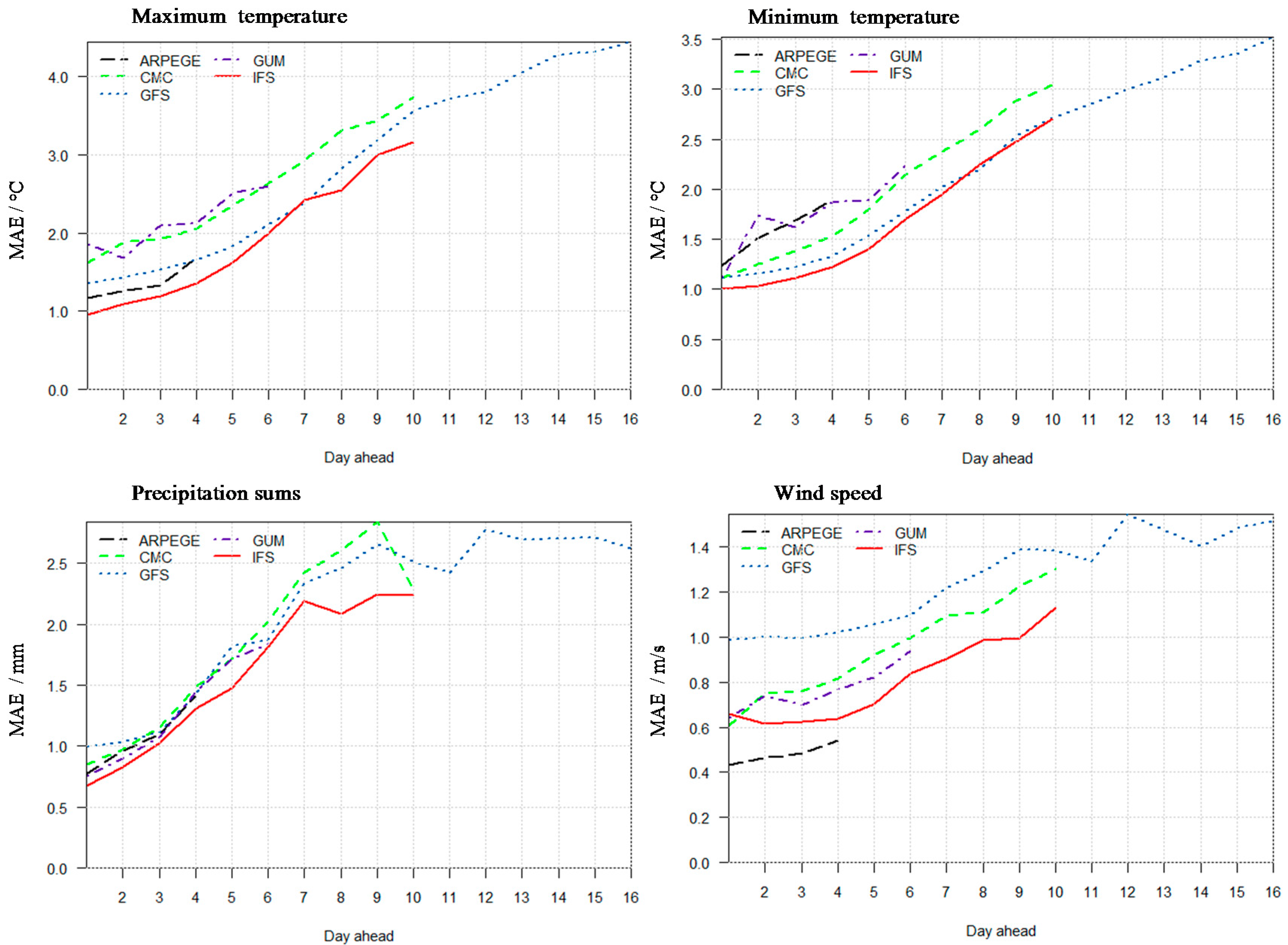
Among the most important meteorological elements for drought forecast by means of SoilClim (www.drought.cz) are maximum and minimum air temperature, precipitation sum, relative humidity, wind speed, and sunshine duration. Validation of the forecast is carried out through comparison of the forecast of these meteorological elements with the reality—the measured values in the network of meteorological stations. The bias of the forecast increases with the length of the forecast, and this bias is pertinent to a given NWP model, as well as a meteorological element and a given part of a year (season). IFS can be regarded as the best NWP model, which shows the lowest model bias for most of the meteorological elements for all the days ahead. On the contrary, the least reliable results are provided by the GFS model.

Air temperature belongs among the best predicable meteorological elements. For maximum air temperature, all the NWP models have a tendency to overestimate values, and this happens mainly in the spring and summer months, which are the most important months for drought monitoring. This may mean a tendency towards slower drying. For the third day ahead, a prediction error (MAE, mean absolute error) varies from 1.19 to 2.10 °C (

Table 2. Validation characteristics (bias and MAE—mean absolute error) of 5 NWP (numerical weather prediction) models for individual seasons (green and asterisk = the best model, red and dash = the worst, estimated based on MAE for annual values) for 3 days ahead.

		YEAR		DJF		MAM		JJA		SON
Element	Model	BIAS	MAE	BIAS	MAE	BIAS	MAE	BIAS	MAE	BIAS	MAE
Maximum temperature	ARPEGE	−0.69	1.33	−0.61	1.29	−1.00	1.47	−0.13	1.29	−1.12	1.28
	CMC	−1.78	1.91	−1.95	2.16	−2.01	2.13	−2.12	2.22	−1.01	1.13
	GFS	−0.90	1.53	−0.62	1.47	−1.70	1.90	−1.59	1.86	0.34	0.89
	GUM -	−1.60	2.10	−0.59	1.46	−1.76	2.05	−1.61	1.98	−2.50	2.97
	IFS *	−0.68	1.19	0.00	1.06	−1.36	1.63	−1.08	1.46	−0.14	0.66
Minimum temperature	ARPEGE -	0.99	1.69	0.45	1.55	0.69	1.49	2.54	2.56	0.06	1.02
	CMC	−0.58	1.38	−2.36	2.70	0.10	0.95	0.29	0.90	−0.36	0.97
	GFS	−0.19	1.22	−0.56	1.47	−0.46	1.09	−0.35	1.28	0.60	1.05
	GUM	1.37	1.62	1.75	2.08	0.99	1.13	1.41	1.42	1.34	1.89
	IFS *	0.62	1.11	−0.46	1.12	0.26	0.87	1.46	1.49	0.64	0.91
Precipitation	ARPEGE	0.27	1.10	0.40	0.63	0.45	1.07	0.12	1.74	0.11	0.88
	CMC -	0.43	1.16	0.48	0.61	0.20	0.96	0.43	1.84	0.63	1.22
	GFS	0.65	1.12	0.56	0.71	0.66	1.10	0.72	1.49	0.68	1.16
	GUM	0.35	1.08	0.48	0.69	0.47	1.01	−0.17	1.52	0.62	1.08
	IFS *	0.17	1.03	0.20	0.45	0.48	1.10	−0.28	1.28	0.38	1.04
Sunshine duration	ARPEGE *	2.84	3.01	1.68	1.88	3.88	4.17	3.28	3.42	2.45	2.52
	CMC	4.03	4.12	2.92	3.04	4.94	5.10	4.22	4.28	4.04	4.04
	GFS -	5.56	5.68	3.10	3.46	6.67	6.78	6.04	6.08	6.30	6.30
	GUM	2.71	3.15	1.65	2.14	3.60	4.07	2.66	3.28	2.95	3.09
	IFS	3.67	3.77	2.24	2.38	4.59	4.76	3.96	4.06	3.48	3.50
Humidity	ARPEGE	4.14	6.32	6.69	6.87	6.61	7.73	0.29	6.08	3.09	4.41
	CMC	4.78	5.49	5.27	5.70	6.20	6.58	4.44	6.06	3.16	3.59
	GFS -	5.37	7.99	5.12	8.98	10.53	10.74	7.98	8.73	−2.33	3.45
	GUM	6.26	6.65	6.02	6.23	8.42	8.80	7.17	7.86	3.16	3.41
	IFS *	−1.45	3.91	−2.67	4.54	2.09	4.02	−1.97	4.05	−2.91	3.34
Wind speed	ARPEGE *	0.19	0.49	0.42	0.59	0.15	0.44	−0.13	0.44	0.37	0.48
	CMC	0.60	0.76	0.54	0.70	0.65	0.75	0.33	0.67	0.88	0.92
	GFS -	0.88	1.00	0.31	0.78	1.36	1.36	0.91	0.92	0.91	0.91
	GUM	0.49	0.70	0.57	0.69	0.53	0.72	0.19	0.60	0.69	0.79
	IFS	0.48	0.62	0.59	0.65	0.49	0.60	0.23	0.54	0.68	0.71

). For 9 days ahead, the error for the IFS model is around 3 °C. As for minimum air temperature, some models overestimate it, while others underestimate it. Error for the third day ahead is slightly lower than in the case of maximum temperature (

Table 3. Validation characteristics of the SoilClim outputs (AWR—relative soil saturation) for individual seasons and 5 NWP models as input (green and asterisk = the best model, red and dash = the worst, estimated based on MAE for annual values) and for the three days ahead forecast. Individual NWP models are explained in Table 1.

		YEAR		DJF		MAM		JJA		SON
Element	Model	BIAS	MAE	BIAS	MAE	BIAS	MAE	BIAS	MAE	BIAS	MAE
AWR 0–100 cm	ARPEGE -	0.54	1.42	0.93	0.95	0.93	2.04	−0.12	1.47	0.69	0.92
	CMC	0.10	1.21	0.15	1.19	0.20	1.50	−0.44	1.33	0.54	0.84
	GFS	0.67	1.30	0.30	1.12	1.21	1.95	0.52	1.26	0.47	0.83
	GUM	0.18	1.30	0.56	0.61	0.46	1.46	−0.10	1.34	0.02	1.37
	IFS *	−0.05	1.08	0.54	0.57	0.40	1.40	−0.88	1.26	0.30	0.83
AWR1 0–40 cm	ARPEGE -	1.37	2.83	2.02	2.09	2.52	3.40	0.00	3.55	1.41	1.77
	CMC	0.40	2.31	0.24	2.76	1.04	2.29	−0.76	2.83	1.03	1.62
	GFS	1.62	2.66	0.63	2.60	3.01	3.55	1.53	2.97	0.83	1.56
	GUM	0.47	2.29	1.20	1.34	1.39	2.07	−0.32	3.00	0.05	2.18
	IFS *	0.18	2.07	1.30	1.36	1.36	2.25	−1.54	2.64	0.72	1.58
AWR2 40–100 cm	ARPEGE	−0.02	0.61	0.20	0.20	−0.14	1.19	−0.20	0.42	0.21	0.40
	CMC	−0.10	0.56	0.09	0.15	−0.36	1.05	−0.23	0.44	0.21	0.38
	GFS *	0.04	0.51	0.07	0.15	0.00	0.96	−0.15	0.36	0.24	0.40
	GUM -	−0.02	0.74	0.13	0.13	−0.17	1.11	0.05	0.47	−0.01	0.89
	IFS	−0.20	0.54	0.04	0.07	−0.24	0.96	−0.45	0.48	0.02	0.43

). For 9 days ahead, the best model—IFS—has an error of only around 2.5 °C.

Precipitation sum is a problematic element. For it, bias increases mainly in the summer months during thunderstorm events when NWP models are not able to determine the exact location and time of its occurrence. Generally, NWP models overestimate precipitation sum falling in the area of the Czech Republic. The error is quite low—around 0.5 mm for 3 days ahead. For the 9 days ahead forecast, the errors are higher than 2.5 mm. Wind speed is among the worst predicable meteorological elements, which is influenced to a large extent by local effect. NWP models possess quite a big bias: they predict by 0.5 to 1.0 m/s higher wind speed compared to station measurements. This is caused by the fact that the models do not contain the roughness of the terrain (or obstacles) to such extent as is reality in the case of the station neighborhood. This is also the reason why wind speed according to models may be closer to reality for drought prediction compared to station measurements. Sunshine duration is difficult to predict during inversions (autumn and spring), when big differences between nearby locations may occur; for this reason, the models show very big positive bias. For the third day, this stands between 3 and 6 h. Relative humidity is overestimated by the models, with exception of IFS. For the third day, the error is from 4 to 8% (Table 2). The least reliable model with regard to relative humidity is GFS.

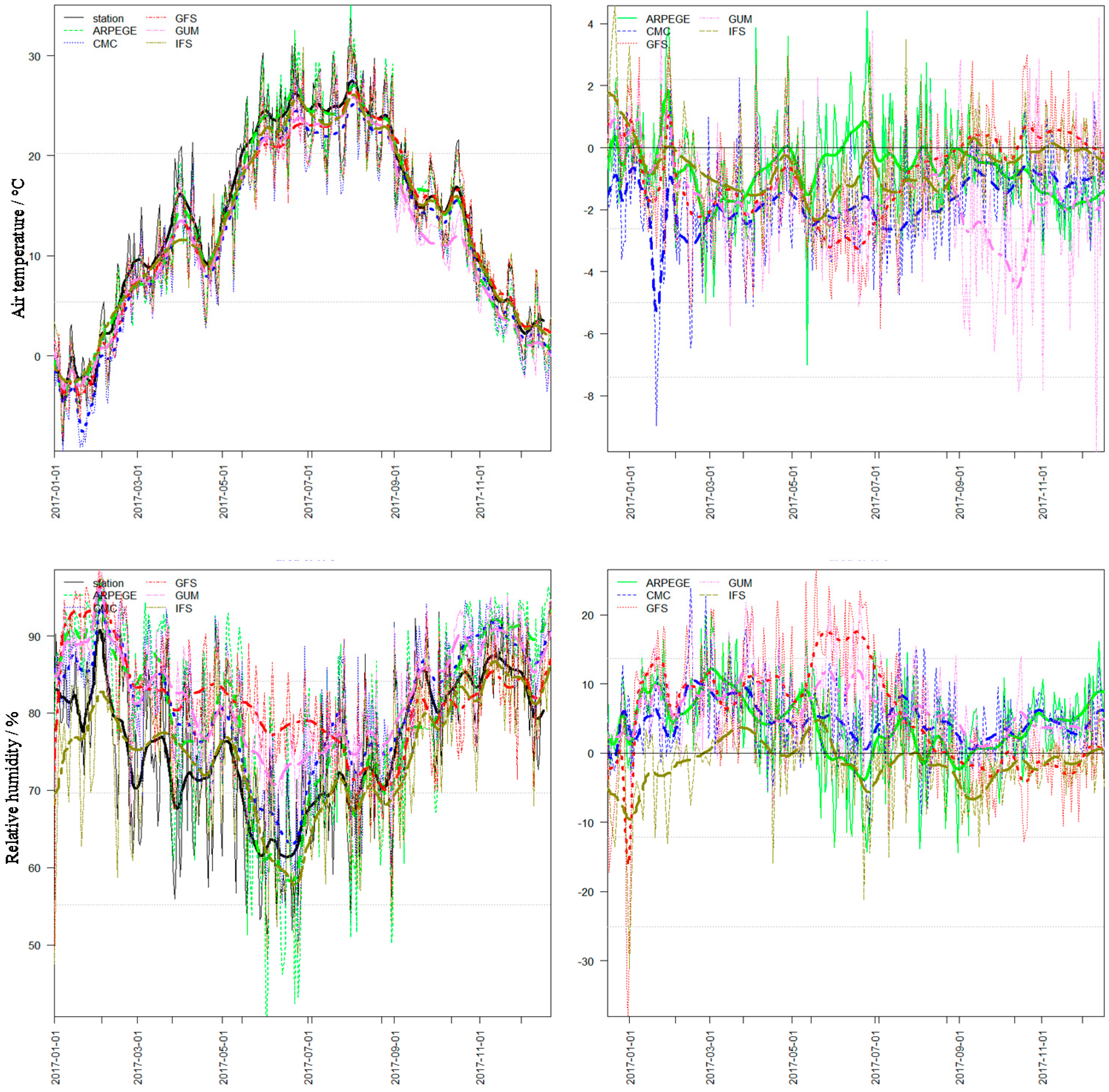
Further in this chapter, we focus only on some specifics of 2017. The forecast for maximum temperature predicted by meteorological models were lower than in reality for all days ahead. The highest negative bias occurred from June to August, especially during days that were warmer than average. Negative bias was from 2 to 4 °C (Figure 4). The beginning and end of the year showed lower bias in terms of maximum air temperatures. What was remarkable was a prediction of the GUM model from 1st September that began to show a significant negative bias for the 1 and 3 days ahead forecasts, but on the other hand, was correct for 2 and 4 days ahead.

In January 2017, a significant cold episode occurred in the Czech Republic, with minimum temperatures dropping below −20 °C. Models for one to four days ahead responded differently. Some models were warmer than was the reality (ARPEGE, GUM), while CMC gave temperature lower by more than 4 °C. In the 9-day forecast, model errors most often ranged from −5 to +5 °C. The difference between the medium-term forecast and the reality of around 10 °C was not an exception. The biggest deviation occurred in the beginning of February for CMC, which expected minimum temperature to be colder by 20 °C.

Practically throughout the whole year, the GFS model showed higher precipitation than occurred in reality (mainly for the 1–4 days ahead forecast). This was most striking at the beginning of July 2017 during a storm situation. The GFS model is generally a wetter model. At the beginning of the dry episode in May 2017, in predictions for 9 days ahead, models consistently believed the following period would have more rain than was the case in reality.

The prediction of relative humidity for 2017 was overestimated according to most of the models (see Figure 5). Closest to reality was the IFS model. In the period of the most severe drought, i.e., from May to July, the predicted relative humidity for 3 days ahead and for the IFS and CMC models was the same low as in reality. On the contrary, other models gave values that were higher by 10–15%, which could lead to underestimation of drought in their cases.

3.2. Validation of NWP Outputs, Station-Based (AVISO) Approach

In the case of the AVISO model, which works with the station network of CHMI, the validation has been performed for the station locations, and only the IFS model has been evaluated (the best NWP model in the sense of predictability bias, as well as in the sense of length—days ahead: comparison with other four NWP models is given above). On the basis of the prepared database of measured meteorological elements from the CHMI station network and the predicted data from the IFS model, the differences were determined for the individual predicted days between the forecast and the measured data (notice the difference between SoilClim and AVISO; while SoilClim works with maps, AVISO works with stations).

The analysis of the forecast data from IFS showed, first of all, a rather significant systematic error caused by a different orography of the predictive model versus reality. The values of the air temperature and the wind speed have the most noticeable dependence of deviations on altitude, and in the case of wind speed, the surrounding area also plays a big role, more precisely, in the openness of the landscape. Other elements have lower dependence on the relief configuration. Despite the fact that the absolute deviations increase with the prediction length, average errors are only very slightly different from zero for the whole season and for all stations. In the case of air temperatures, average deviations vary between +1 and −1 °C, but of course, extremes of difference may also occur in certain situations, but this applies only to extreme situations and to the predictive length of 6 or more days. Air humidity is also a highly variable feature with high sensitivity to local conditions and altitude dependence. The amount of global radiation is then systematically underestimated by up to 12% by the IFS model on bright days in the summer months, and the wind speed is greatly underestimated in the case of strong wind at higher altitudes. Precipitation totals have the most variations in the 0 to 2 mm category, but only due to the large number of non-precipitated cases. Average daily precipitation total deviations show a trend of higher overestimation at lower altitudes and underestimation of precipitation at higher altitudes. This is determined by the IFS model properties.

Comparing the deviations of the meteorological elements in the daily scale with synoptic situations can serve as a guideline within which situations large differences in forecasts can be expected. The biggest problems are logically found during cyclonic and dynamic weather types. During storm situations, there may be significant underestimation of precipitation sums in the forecast, as well as inaccurate localization of intense rainfall events. On the other hand, for example, the highest frequency of significant deviations in the forecast of air temperature is typical for anticyclonic weather patterns.

3.3. Validation of Drought Characteristics, SoilClim Outputs

Again, as in the case of input meteorological elements, the following comparison is given with regard to a general overview for the whole Czech Republic (spatial values aggregated from maps, i.e., interpolated values), focusing mainly on the past year, 2017.

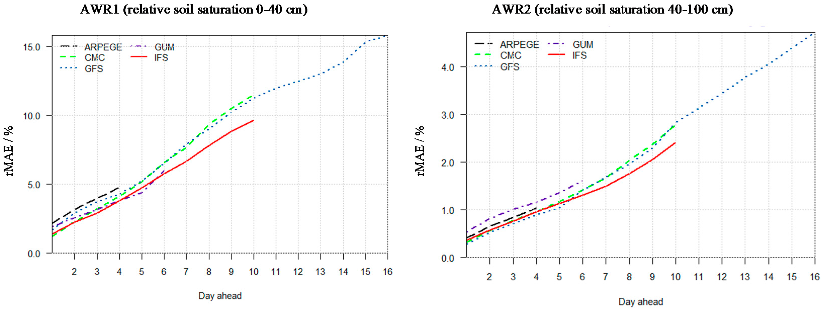
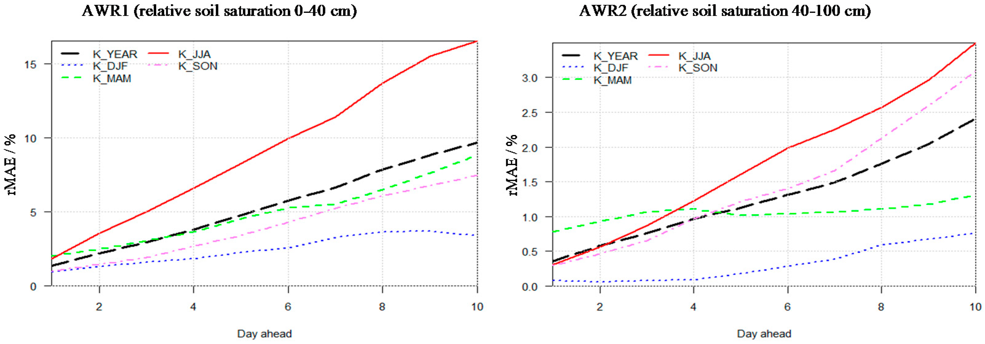
It is only a combination of individual meteorological elements that shows real reliability of the outputs of a given NWP model. For the whole soil profile of 0–100 cm, differences among NWP models for the first four days ahead are very small. As for AWR—relative soil saturation (in which 0% stands for saturation at wilting point and 100% for field capacity), we again find again IFS to be the best NPW model, with an error (relative MAE) of about 0.5% for the first day ahead forecast and 1.08% for the third one (Table 3). In medium-range outlook (9 days ahead), the individual NWP models give more different results. The IFS NWP model still holds the best results with MAE of about 4.7%. The other two long forecasts (CMC and GFS) give an average difference from reality of 5.5%. Most of the models have a tendency to rather overestimate soil moisture, and this is especially valid for fifth to ninth day ahead. There is a noticeable difference in forecast accuracy for relative humidity between upper and deeper soil layers. The upper soil layer is very sensitive and shows higher deviations compared to reality, which is caused mainly by higher uncertainty in precipitation estimation. MAE values for the 0–40 cm profile are between 2.07% and 2.83% for the third day ahead (see Table 3 and Figure 6). For the 40–100 cm profile, the MAE is between 0.54% and 0.74%.

The results for other drought characteristics are similar to AWR. Drought intensity is divided into 6 categories. The evaluation of a forecast is quantified as the percentage difference between the averaged category of drought over the Czech Republic and that forecast. For the whole soil profile of 0–100 cm, the NWP model, IFS, is again the most accurate one, with its reliability almost 98% for three days ahead and almost 97% for 9 days ahead. A general rule about whether the NWP models overestimate or underestimate drought was not found in our results; NWP models differ among themselves, and there is also a difference among the individual seasons. Thus, the results are pertinent to random fluctuations, this fact being caused also thanks to relatively low errors in drought prediction.

The prediction of drought by means of the relative soil saturation (AWR), a category of the intensity of drought (AWP) and the deficit of soil moisture (AWDMED) in the year 2017, gave similar and very good results. In the surface profile up to 40 cm, the difference between the prediction and reality was bigger in the first half of the year 2017, when drought was more intense. On the contrary, in the second half of the year, the land was fully saturated, and the share of conventional rainfall declined, so the prediction was very similar to reality.

The drought episode was most intensive from half way through June to the middle of July. In this period, most of the prediction models forecast (1–9 days ahead) more intensive drought than in reality (see Figure 7 for an example of the IFS model). The exception was the GFS model, which overestimated convective precipitation and therefore predicted quicker soil moisture replenishment. On the contrary, at the beginning of the dry period from May to June 2017, models tended to predict more soil moisture than there actually was in the upper soil profile. In the deeper profile, the model forecast for 1–8 days ahead was drier than in reality from the beginning of May 2017. The situation at the beginning of November 2017 was interesting, when the models anticipated a quicker replenishment of soil moisture in the profile of 40–100 cm than actually happened in reality.

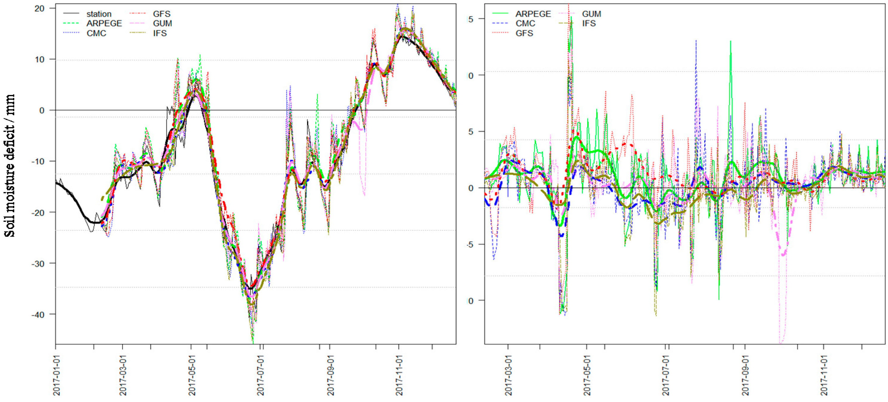
Figure 8 shows the deviation from the reality of the forecast for soil moisture deficit for the whole profile of 0–100 cm for the 3 days ahead during the year 2017. It is evident that deviations of the forecast from reality have not been overcome; in the daily scale, a difference of more than 15 mm, and in the 30-day average, 3 mm of soil moisture deficit for whole profile, with similar results also achieved in the upper profile. The deeper soil profile shows even lower deviations.

The fluctuations are similar when we compare the results for the whole soil profile (0–100 cm) or the upper profile (0–40 cm), while for the deeper profile (40–100), the values are much smoother. At the same time, various drought characteristics show similar fluctuations for a given soil profile (there are only small differences between each other), which is why we showed results only for selected drought characteristics.

3.4. Validation of Drought Characteristics, AVISO Outputs

As mentioned above, AVISO is paired with the IFS model, having this in common with the SoilClim model, so the results are well comparable in this sense. While previous validation was performed on a 500 m grid (for SoilClim), here, we give the information again in the form of stations.

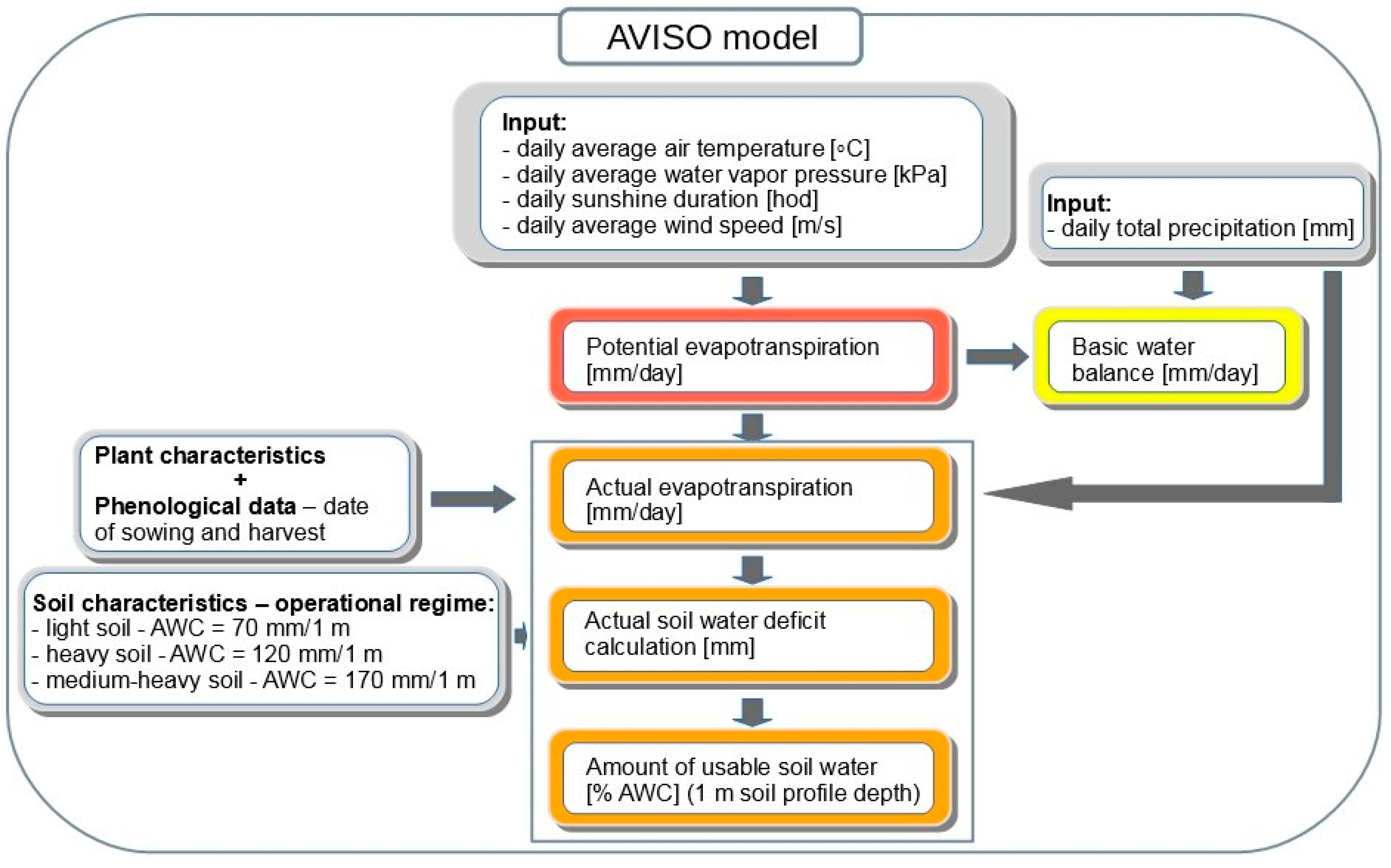
With the AVISO model, we analyzed the forecasts for the period of 2014–2016 retrospectively, and for 2017, continuously (but still in experimental test mode). The database contains an input data set of actual meteorological data measured at 198 stations of CHMI and the forecast IFS data in daily steps for four years (eight days ahead in 2014, 2015 and nine days in 2016, 2017).

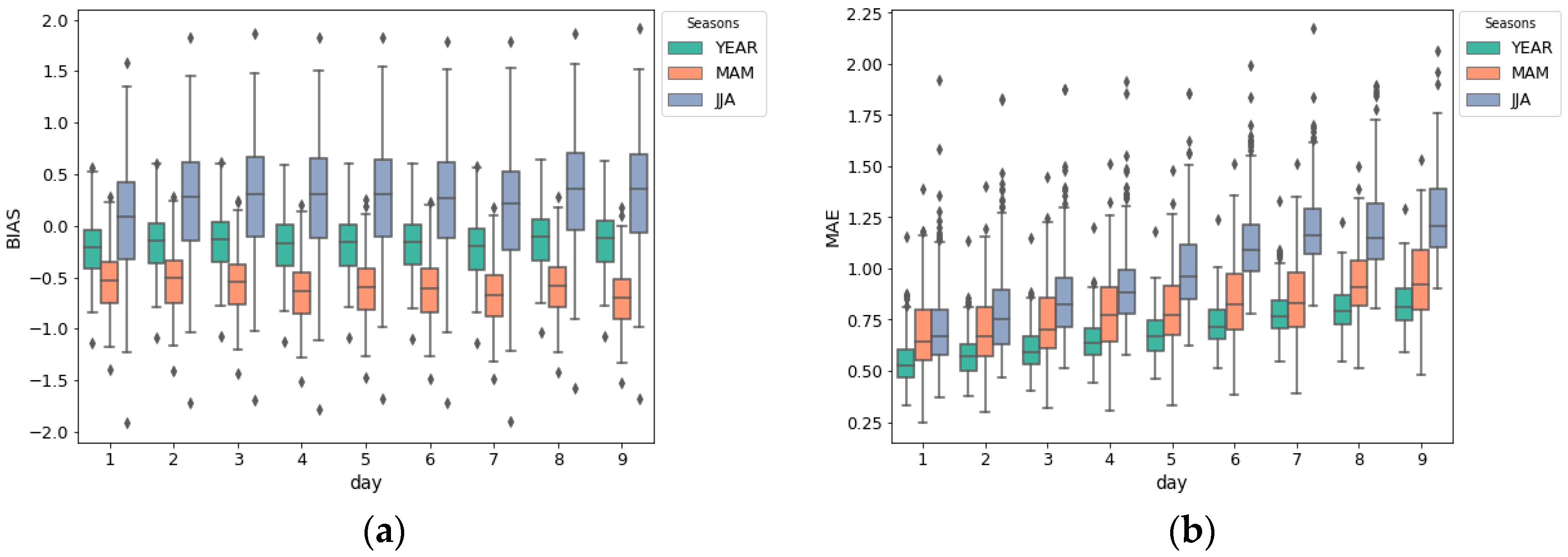
The evapotranspiration as deficit component is needed for soil water content determination. The potential evapotranspiration is used primarily and for general assessment of the influence of climatic conditions in the Drought monitoring system at CHMI. From the assessment of the mean differences in potential evapotranspiration calculated from the measured and predicted data, there is a clear increase in the forecast deviation with each predicted day, as shown in Figure 9. These differences are low for the year and the spring season (MAM); more significant differences are evident in the forecast for the sixth and next days and also in the summer season (JJA). In accordance with bias, the forecast generally overestimates the evaporation. In the spring months, the prediction of potential evapotranspiration is underestimated on average.

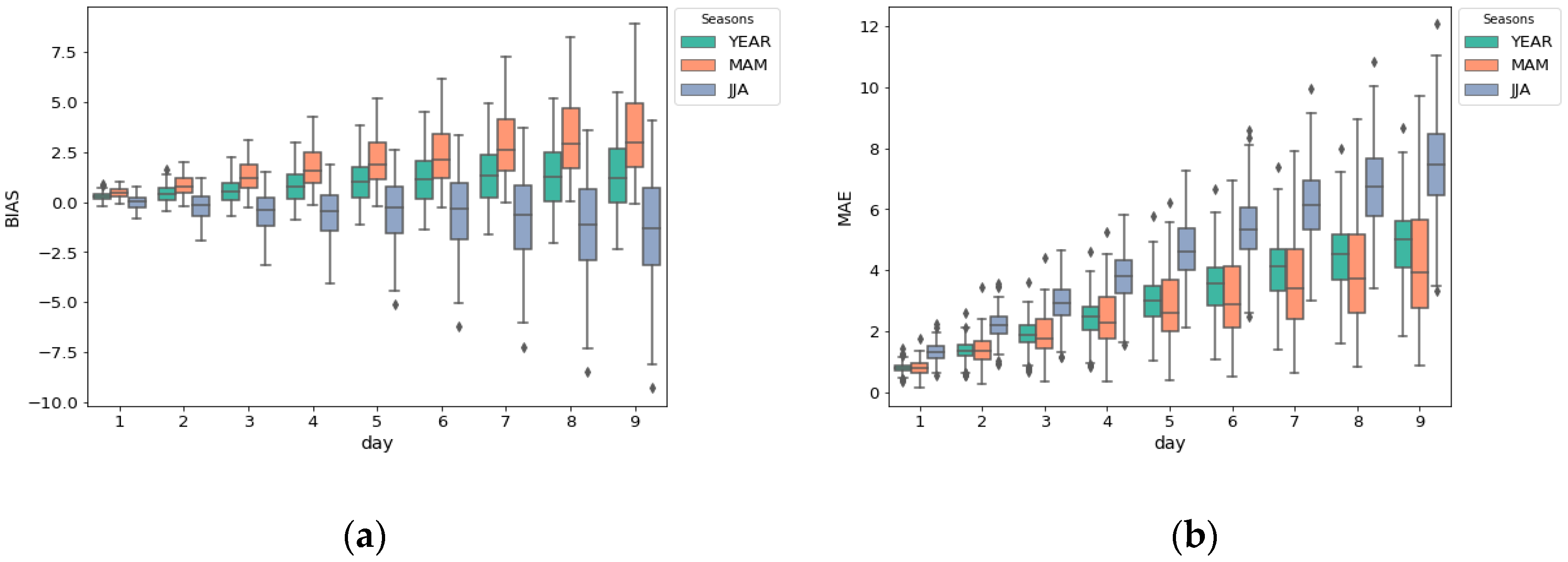
The prognosis of the state of the soil water content is calculated from the starting current state on the calculation day and is followed in the daily steps of balancing the consumption and supply of water to the soil based on the calculation of the model from the forecast data. As a result, the increasing number of days of prediction leads to increasing mean values of the deviations of predictions and real values. As shown in Figure 10b, the average daily difference of soil water content for the 9th day of the forecast in the summer period is about 7% AWC. In the spring season and throughout the year, average differences are lower. The BIAS analysis (Figure 10a) shows that the forecast tends to predict higher soil water content in the spring months and lower values in the summer.

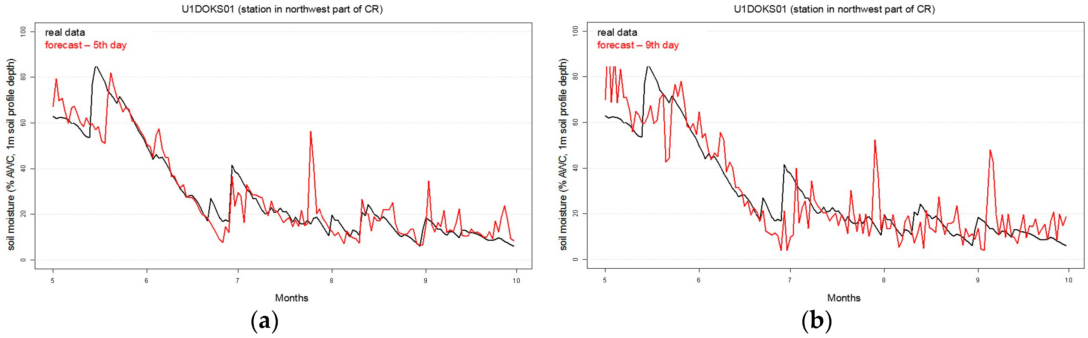
An example of the soil water content change on the agrometeorological observatory Doksany calculated from operative and forecast data is shown in Figure 11 (to illustrate the difference for a particular location). With a dynamic type of weather, the results of the calculation from the forecast data and calculation from the measured can also differ significantly. Precipitation has a large impact on soil water content. Unfortunately, it is difficult to predict precipitation in terms of total and time and location of occurrence in some types of weather conditions. In the graphs, this can be observed by gauging the results of the model for operational and predictive data. For this reason, it is appropriate to use a set of models for the optimal medium-term precipitation prediction. In the optimal case, an improved estimation of precipitation leads to the correct determination of the water content in the soil.

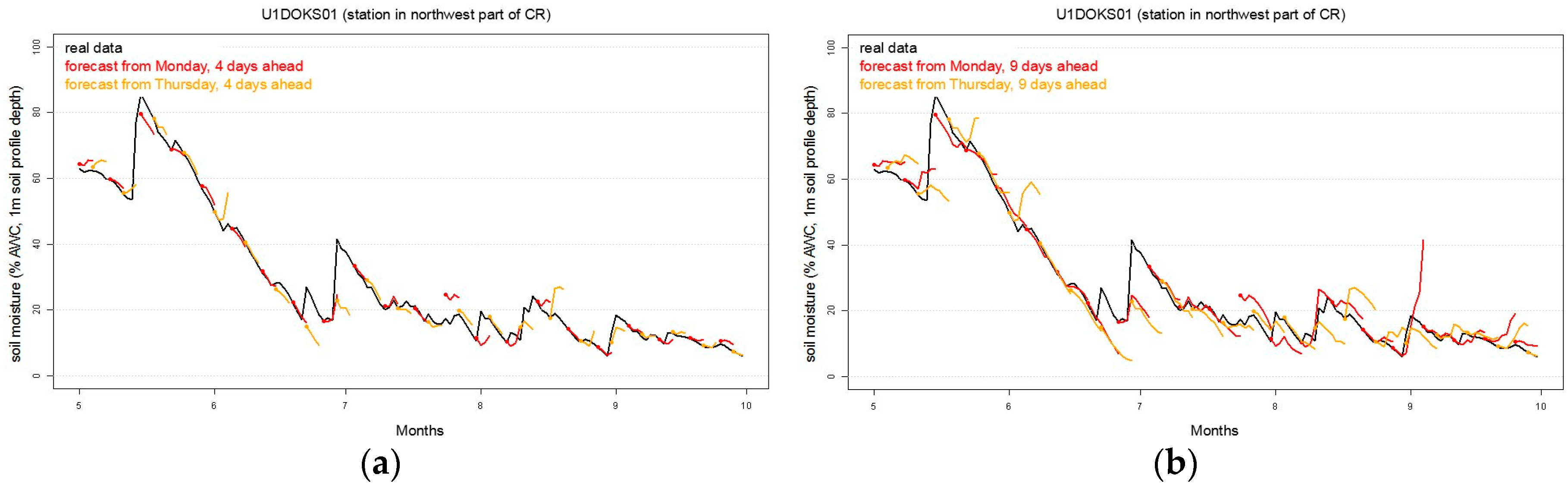
In the Czech Republic, the labour week starts on Monday. This is why the weather forecast from Monday is important for agriculture and field work planning. Thursday is also important for planning Friday’s work, when the weather is going to change dramatically on the weekend. With this in mind, the figures below (Figure 12) show the AVISO output (soil water content in % of available water capacity) computed from measured data and forecast data from Monday and Thursday for four and nine days. The SoilClim–based drought forecast is issued by www.drought.cz operationally (daily), and for practical reasons it was decided to issue the AVISO forecast daily as well to avoid decay in the forecast reliability.

4. Discussion

The novelty of the presented approach is, first of all, the creation of the ensemble prediction system for estimation of soil moisture and drought intensity based on several NWP models. Adding to these different NWP models, we apply two different models of soil moisture, SoilClim and AVISO. This gives a user a wide range of outputs, from which the uncertainty in future development can be seen (when the results do not coincide, but depart). Thanks to the fact that not only are drought characteristics given to users but also input meteorological elements (air temperature, precipitation, wind speed, relative humidity, and sunshine duration), such wider context helps to better understand the current situation. The research questions related to the drought forecasting featured also in the recent set of priority topics [9] in particular: How well have the current climate forecast systems done in predicting recent droughts over short to seasonal timescales? and What are the predictabilities of droughts and are these regionally specific? The presented study provides answers specific for the Czech Republic and Central Europe in General. The early drought warning has been implemented in some of developed economies in an effort to cut on enormous damages that drought can cause, e.g., to extensive rangelands in the US mid–west (e.g., [29]). The forecast and prediction efforts take various forms from long–term forecast, through medium–term forecasting [29] to short–term high resolution forecast considering an ensemble of numerical weather prediction models like those presented in this paper. Whilst, Ref. [30] showed that in some world regions severe drought conditions are associated with more than 70% of ENSO events; this is not the case in the region presented in this study, and, currently, seasonal and even annual drought forecasts are not sufficiently accurate to guarantee their use. However, given general atmospheric circulation patterns, other atmospheric factors are may be able to explain drought occurrence at regional scales (for example, storm track frequency and direction and blocking conditions [31,32,33,34]).

The year 2017 can be considered as an ideal case for the validation of the drought forecast system and evaluating its assets. The drought conditions in the Czech Republic in 2017 showed regionally very diverse pattern. Drought affected different regions during different times of the year, with a few dry events consisting of several shorter episodes. Central Moravia was hit by drought in spring, southern Bohemia and Moravia in summer. Wrong forecast of these individual events would negatively affect the forecast score on the national level. Despite regional differences among the individual NWP models, the prediction of soil moisture and drought intensity–based IFS model of ECMWF is the most successful in the long term, and users should rely on it most. Other NWP models (GFS, CMC, ARPEGE, and GUM) show lower forecast scores that vary for individual parameters during different parts of the year. To consider this fact in the forecast system, we present biases of all models within last 1 and 3 weeks on the web portal (www.drought.cz). This allows users to check the most recent reliability of the forecast for a given parameter and model.

The forecast from June to August 2017 shows increased bias. It is caused by high precipitation amounts due to the local convective precipitation that is able to significantly affect soil moisture. The reliability of the drought forecast is high, even higher than forecast for the individual meteorological parameters. This is due to the fact that relatively large amount of precipitation (or energy) is required to change the state of the soil.

The drought monitoring system itself offers a wide range of other characteristics related to drought as well, and the combination with the remote sensing data provides another hope for the forecast accuracy improvement. However, it is beyond the scope of this article to analyze all of these other drought characteristics, and we only limit ourselves to a mention of their possible use in the forecast. Our aim was to present the skill of the forecast system for soil moisture and drought intensity and demonstrate its sense for user decision making.

It is, however, obvious that the presentation of the forecast in the form of understandable maps is fully compatible with the original product, as the SoilClim (and its 500 m grid) is much more user friendly compared to the station–based approach of AVISO, which accounts for 198 individual weather stations. The validation of the forecast system could be also performed for these individual regions/stations. The preliminary analysis performed on the smaller scales indicates that while biases grow, the reliability and rank of the individual NWP models remains the same.

5. Conclusions

We have created an ensemble prediction system consisting of five global NWP models and two soil models, SoilClim (www.drought.cz) and AVISO (www.chmi.cz), to forecast soil moisture and drought intensity. The system offers a wide range of products whose level of (dis)agreement informs users about the uncertainty of the forecast. To obtain a wider context and better understating of the drought development up to several days, the system provides a forecast of drought characteristics and meteorological variables too. The results may be thus interesting, not only for users from agricultural communities but for other sectors as well. The development and implementation of the system have been started through suggestion of farming community, which demanded not only near-real time product but a future oriented approach, which allows sufficient time for drought response.

The application of both soil models leads to comparable results in the forecast. Among the NWP models, the ECMWF IFS model shows the best score in the forecasted parameters. The scores of the models vary among parameters and periods. Users of the forecast system are thus informed of the most recent biases within the last 1 and 3 weeks together with the forecast itself.

The validation has been primarily performed using relative soil saturation—AWR (%) and the deficit of soil moisture—AWDMED (mm). For these two variables, we compared the soil model estimates based on NWP driven forecasts with the model runs based on observed data (i.e., via the hind-casting model). AWR and AWDMED are used, as they can be compared more-or-less directly with measurements and allow independent ground verification of the system. However, the main output used by the stakeholders is the intensity of drought (AWP). This represents probabilistic interpretation of the actual AWR value in relation to all AWR values occurring at the given grid between 1961 and 2010 during the same period of year. The AWP values are then provided as the principal forecast map (www.drought.cz), as they allow for the interpretion of the current soil moisture situation with respect to the values that should be expected.

In this paper, we have shown that the developed ensembles prediction system delivers accurate and reliable forecasts of the drought conditions up to several days, and it can be used as a basis for decision making by user groups ranging from individual farmers to experts of local and notional authorities in various sectors.

References

1. Enenkel, M.; See, L.; Karner, M.; Álvarez, M.; Rogenhofer, E.; Baraldès-Vallverdú, C.; Lanusse, C.; Salse, N. Food security monitoring via mobile data collection and remote sensing: Results from the Central African Republic. PLoS ONE 2015, 10, e0142030. [Google Scholar] [CrossRef] [PubMed] [Green Version]
2. Tadesse, T.; Haigh, T.; Wall, N.; Shiferaw, A.; Zaitchik, B.; Beyene, S.; Berhan, G.; Petr, J. Linking seasonal predictions to decision-making and disaster management in the Greater Horn of Africa. Bull. Am. Meteorol. Soc. 2016, 97, ES89–ES92. [Google Scholar] [CrossRef]
3. Wilhite, D.A.; Pulwarty, R.S. (Eds.) Drought and Water Crises. Integrating Science, Management, and Policy; CRC Press: Boca Raton, FL, USA; London, UK; New York, NY, USA, 2017; pp. 461–480. [Google Scholar]
4. Oguntoyinbo, J.S. Drought prediction. Clim. Chang. 1986, 9, 79. [Google Scholar] [CrossRef]
5. Ceppi, A.; Ravazzani, G.; Corbari, C.; Salerno, R.; Meucci, S.; Mancini, M. Real-time drought forecasting system for irrigation management. Hydrol. Earth Syst. Sci. 2014, 18, 3353–3366. [Google Scholar] [CrossRef] [Green Version]
6. Dutra, E.; Pozzi, W.; Wetterhall, F.; Di Giuseppe, F.; Magnusson, L.; Naumann, G.; Barbosa, P.; Vogt, J.; Pappenberger, F. Global meteorological drought—Part 2: Seasonal forecasts. Hydrol. Earth Syst. Sci. 2014, 18, 2669–2678. [Google Scholar] [CrossRef] [Green Version]
7. Wetterhall, F.; Winsemius, H.C.; Dutra, E.; Werner, M.; Pappenberger, F. Seasonal predictions of agro-meteorological drought indicators for the Limpopo basin. Hydrol. Earth Syst. Sci. 2015, 19, 2577–2586. [Google Scholar] [CrossRef]
8. Mishra, A.K.; Singh, V.P. Drought modeling—A review. J. Hydrol. 2011, 403, 157–175. [Google Scholar] [CrossRef]
9. Trnka, M.; Balek, J.; Semerádová, D.; Hlavinka, P.; Možný, M.; Štěpánek, P.; Zahradníček, P.; Bartošová, L.; Bláhová, M.; Skalák, P.; et al. Czech Drought Monitoring System and the role of drought reporters. Clim. Res. 2018. submitted. [Google Scholar]
10. Allen, R.G.; Pereira, L.S.; Raes, D.; Smith, M. Crop Evapotranspiration. Guidelines for Computing Crop Water Requirements; FAO Irrigation and Drainage Paper No. 56; Food and Agriculture Organization (FAO): Roma, Italy, 1998; 301p. [Google Scholar]
11. Hlavinka, P.; Trnka, M.; Balek, J.; Semerádová, D.; Hayes, M.; Svoboda, M.; Eitzinger, J.; Mozny, M.; Fischer, M.; Hunt, E.; et al. Development and evaluationof the SoilClim model for water balance and soil climate estimates. Agric. Water Manag. 2011, 98, 1249–1261. [Google Scholar] [CrossRef]
12. Trnka, M.; Brázdil, R.; Možný, M.; Štěpánek, P.; Dobrovolný, P.; Zahradníček, P.; Balek, J.; Semerádová, D.; Dubrovský, M.; Hlavinka, P.; et al. Soil moisture trends in the Czech Republic between 1961 and 2012. Int. J. Climatol. 2015, 35, 3733–3747. [Google Scholar] [CrossRef]
13. Trnka, M.; Kocmankova, E.; Balek, J.; Eitzinger, J.; Ruget, F.; Formayer, H.; Hlavinka, P.; Schaumberger, A.; Horakova, V.; Mozny, M.; et al. Simple snow cover model for agrometeorological applications. Agric. For. Meteorol. 2010, 150, 1115–1127. [Google Scholar] [CrossRef]
14. Dingman, S.L. Physical Hydrology, 2nd ed.; Prentice-Hall: Upper Saddle River, NJ, USA, 2002; 646p. [Google Scholar]
15. Panagos, P.; Jones, A.; Bosco, C.; Senthil Kumar, P.S. European digital archive on soil maps (EuDASM): Preserving important soil data for public free access. Int. J. Digit. Earth 2011, 4, 434–443. [Google Scholar] [CrossRef]
16. Fan, Y.; Li, H.; Migues-Macho, G. Global patterns of ground water table depth. Science 2013, 339, 940–943. [Google Scholar] [CrossRef] [PubMed]
17. Trnka, M.; Brázdil, R.; Balek, J.; Semerádová, D.; Hlavinka, P.; Možný, M.; Štěpánek, P.; Dobrovolný, P.; Zahradníček, P.; Dubrovský, M.; et al. Drivers of soil drying in the Czech Republic between 1961 and 2012. Int. J. Climatol. 2014. [Google Scholar] [CrossRef]
18. Zalud, Z.; Hlavinka, P.; Prokeš, K.; Semerádová, D.; Balek, J.; Trnka, M. Impacts of water availability and drought on maize yield—A comparison of 16 indicators. Agric. Water Manag. 2017, 188, 126–135. [Google Scholar] [CrossRef]
19. Gardner, C.M.K. The MORECS Discussion Meeting (April 1981); Report No. 78; Institute of Hydrology: Bracknell, UK, 1981; 58p. [Google Scholar]
20. Gardner, C.M.K.; Field, M. An evaluation of the success of MORECS, a meteorological model, in estimating soil moisture deficits. Agric. Meteorol. 1983, 29, 269–284. [Google Scholar] [CrossRef]
21. Hough, M.; Jones, R. The United Kingdom Meteorological Office rainfall and evaporation calculation system: MORECS version 2.0—An overview. Hydrol. Earth Syst. Sci. 1997, 1, 227–239. [Google Scholar] [CrossRef]
22. Hough, M.; Palmer, S.; Weir, A.; Lee, M.; Barrie, I. The Meteorological Office Rainfall and Evaporation Calculation System: MORECS Version 2.0; Meteorological Office Bracknell, Meteorological Office Wolverhampton: Bracknell, UK, 1997; 82p.
23. Thompson, N.; Barrie, I.A.; Ayles, M. The meteorological office rainfall and evaporation calculation system —MORECS. Agric. Water Manag. 1983, 6, 297–306. [Google Scholar]
24. Kohut, M. Water Balance of the Agricultural Landscape. Ph.D. Thesis, Mendel University in Brno, Brno, Czech Republic, 2007; 128p. (In Czech). [Google Scholar]
25. Kohut, M.; Roznovsky, J.; Chuchma, F. The long-term soil moisture reserve variability in the Czech Republic based on the AVISO model. In Proceedings of the Sustainable Development and Bioclimate: Reviewed Conference, Stará Lesná, Slovakia, 5–8 October 2009; Pribullová, Bičarová, Eds.; Slovak Academy of Sciences: Bratislava, Slovakia, 2009; pp. 160–161, ISBN 978-80-900450-1-9. [Google Scholar]
26. Kohut, M.; Vitoslavsky, J. Agrometeorological computer and information system—The possibility of its use. In Agro-Meteorological Forecasts and Models; Litschman: Velke Bilovice, Czech Republic, 1999; pp. 53–61. (In Czech) [Google Scholar]
27. Štěpánek, P.; Zahradníček, P.; Farda, A. Experiences with data quality control and homogenization of daily records of various meteorological elements in the Czech Republic in the period 1961–2010. Időjárás 2013, 117, 123–141. [Google Scholar]
28. Stepanek, P.; Zahradnicek, P.; Farda, A.; Skalak, P.; Trnka, M.; Meitner, J.; Rajdl, K. Projection of drought-inducing climate conditions in the Czech Republic according to Euro-CORDEX models. Clim. Res. 2016, 70, 179–193. [Google Scholar] [CrossRef]
29. Tadesse, T.; Wardlow, B.D.; Hayes, M.J.; Svoboda, M.D.; Brown, J.F. The Vegetation Outlook (VegOut): A new method for predicting vegetation seasonal greenness. GISci. Remote Sens. 2010, 47, 25–52. [Google Scholar] [CrossRef]
30. Vicente-Serrano, S.M.; López-Moreno, J.I.; Gimeno, L.; Nieto, R.; Morán-Tejeda, E.; Lorenzo-Lacruz, J.; Beguería, S.; Azorin-Molina, C. A multi-scalar global evaluation of the impact of ENSO on droughts. J. Geophys. Res. Atmos. 2011, 116, D20109. [Google Scholar] [CrossRef]
31. García-Herrera, R.; Paredes, D.; Trigo, R.M.; Barriopedro, D.; Mendes, M.A. The outstanding 2004/05 drought in the Iberian Peninsula: Associated atmospheric circulation. J. Hydrometeorol. 2007, 8, 483–498. [Google Scholar] [CrossRef]
32. Liberato, M.L.R.; Ramos, A.M.; Gouveia, C.M.; Trigo, R.M.; Santo, F.E. Exceptionally extreme drought in Madeira Archipelago in 2012: Vegetation impacts and driving conditions. Agric. For. Meteorol. 2017, 232, 195–209. [Google Scholar] [CrossRef]
33. Ramos, A.M.; Nieto, R.; Tomé, R.; Liberato, M.L.R.; Lavers, D.A. Atmospheric rivers moisture sources from a Lagrangian perspective. Earth Syst. Dyn. 2016, 7, 371–384. [Google Scholar] [CrossRef]
34. Santos, J.; Corte-Real, J.; Leite, S. Atmospheric large-scale dynamics during the 2004/2005 winter drought in Portugal. Int. J. Climatol. 2007, 27, 571–586. [Google Scholar] [CrossRef]
Figure 1. (a) Diagram of data processing in the soil moisture and drought intensity model SoilClim; (b) current area of interest covered by the weekly drought monitoring efforts.
Geosciences 08 00104 g001
Figure 2. Scheme of data processing in the AVISO agrometeorological model.
Geosciences 08 00104 g002
Figure 3. Diagram of data processing in forecast mode of the AVISO agrometeorological model run.
Geosciences 08 00104 g003
Figure 4. MAE (mean absolute error) as difference between forecast and measured meteorological element for maximum air temperature (upper left), minimum air temperature (upper right), precipitation sums (bottom left), and wind speed (bottom right) for the given number of days ahead (horizontal axis).
Geosciences 08 00104 g004
Figure 5. (Top left): maximum temperature (in °C) predicted by five meteorological models for 3 days ahead and reality (black) in the Czech Republic in the year 2017. (Top right): maximum temperature differences of the NPW outputs with regard to reference series (reality based on station data interpolated into maps). Thick lines: values smoothed with 30-day low-pass Gaussian filter. (Bottom): the same as above but for relative humidity (in %).
Geosciences 08 00104 g005
Figure 6. Relative MAE (mean absolute error), as difference of forecast and AWR (relative soil saturation) in two depths: (left) upper (0–40 cm) soil profile, and (right) deeper (40–100 cm) soil profile.
Geosciences 08 00104 g006
Figure 7. Relative MAE for IFS for individual seasons, upper soil profile (left) and deeper soil profile (right), for 10 days ahead (black line: YEAR, blue—DJF—winter, green—MAM—spring, red—JJA—summer, purple—SON—autumn).
Geosciences 08 00104 g007
Figure 8. (Left) Comparison of the meteorological forecast of the soil moisture deficit in the whole profile (0–100 cm) provided by 5 NWP models for 3 days ahead and reality (black) in the Czech Republic in the year 2017. (Right) Differences of the NPW outputs with regard to reference series (reality based on station data interpolated into maps). Thick lines: values smoothed with 30-day low-pass Guassian filter.
Geosciences 08 00104 g008
Figure 9. BIAS (a) and MAE (mean absolute error) (b) evaluated from daily differences of values of potential evapotranspiration calculated from forecast data and real measured data for year (YEAR), spring (MAM—March, April, May) and summer season (JJA—June, July, August) from the 1st to 9th day of the forecast in the year 2017.
Geosciences 08 00104 g009
Figure 10. BIAS (a) and MAE (mean absolute error) (b) evaluated from daily differences of values of soil water content (in % AWC, grassland, 1 m soil depth with AWC = 170 mm) calculated from forecast data and real measured data for year (YEAR), for the spring (MAM—March, April, May) and summer season (JJA—June, July, August) from the 1st to 9th day of the forecast in the year 2017.
Geosciences 08 00104 g010
Figure 11. The course of soil moisture content (in % AWC) calculated from measured meteorological station data and forecast data for the 5th (a) and 9th (b) day of the forecast in the evaluated part of the year 2017 at Doksany station.
Geosciences 08 00104 g011
Figure 12. The course of soil moisture content (in % AWC) calculated from measured meteorological station data and the 4th day (a) and 9th day (b) forecasts developed periodically on Mondays and Thursdays in the evaluated part of the year 2017 at Doksany station.
Geosciences 08 00104 g012