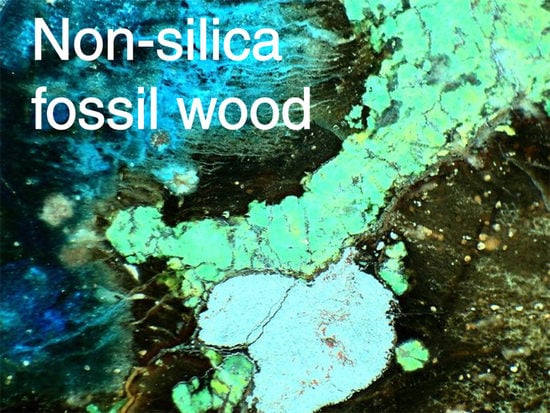
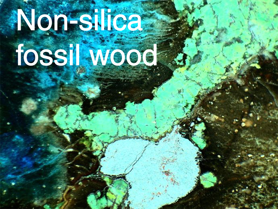
Mineralogy of Non-Silicified Fossil Wood


Abstract
1. Introduction
Previous Work
2. Analytical Methods
3. Carbonate Minerals: Calcite and Dolomite
Dolomite Wood
4. Calcium Phosphate
5. Iron Minerals
5.1. Iron Oxides and Hydroxides
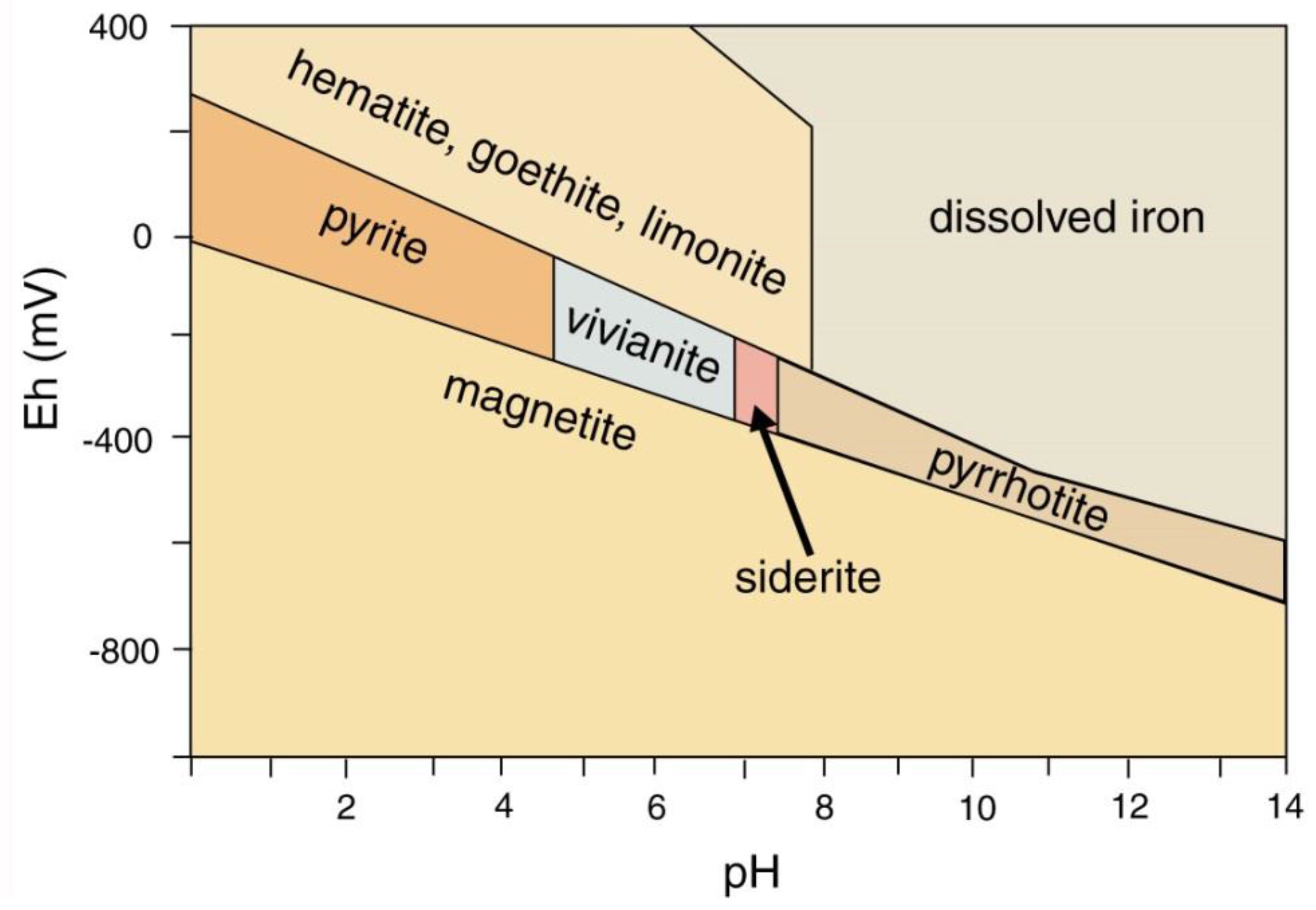
5.2. Iron Carbonate
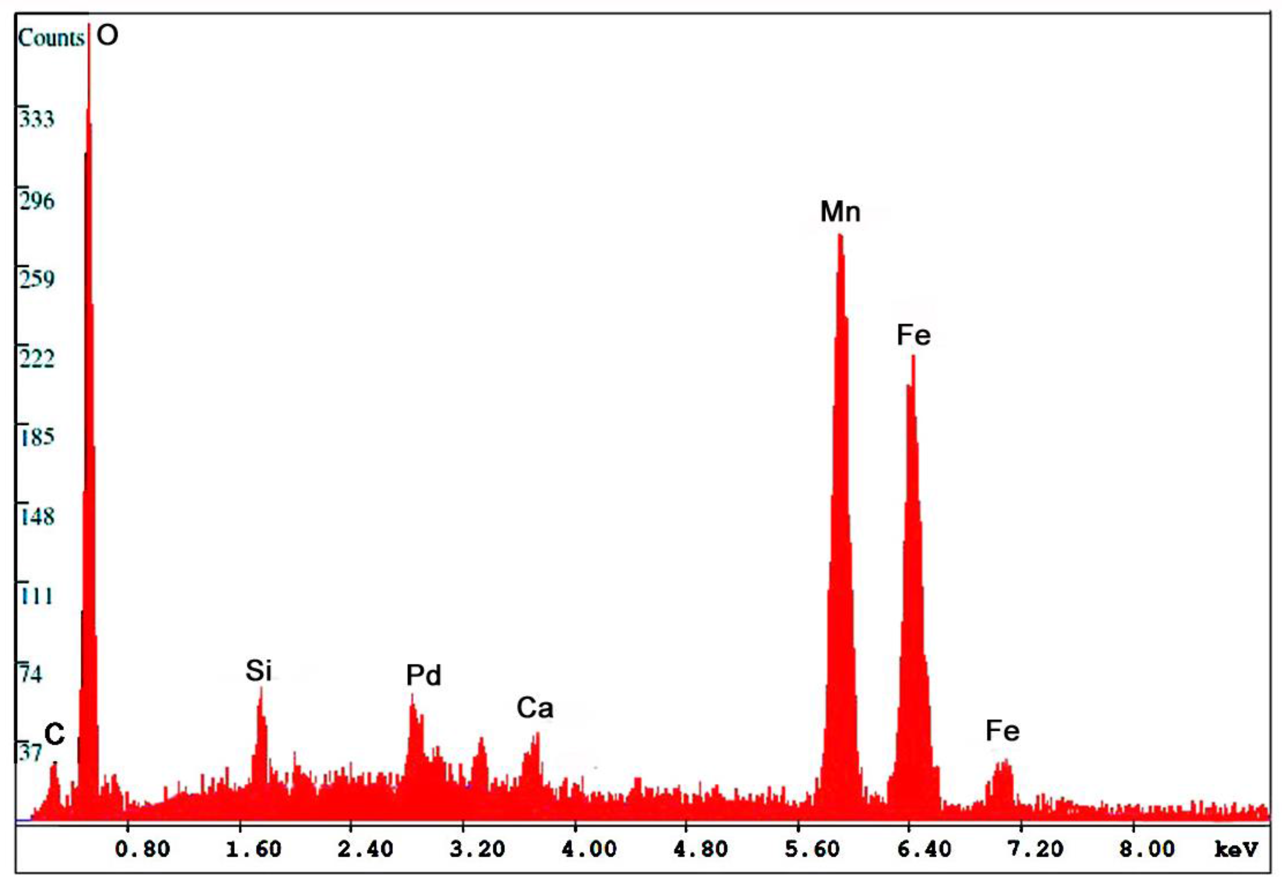
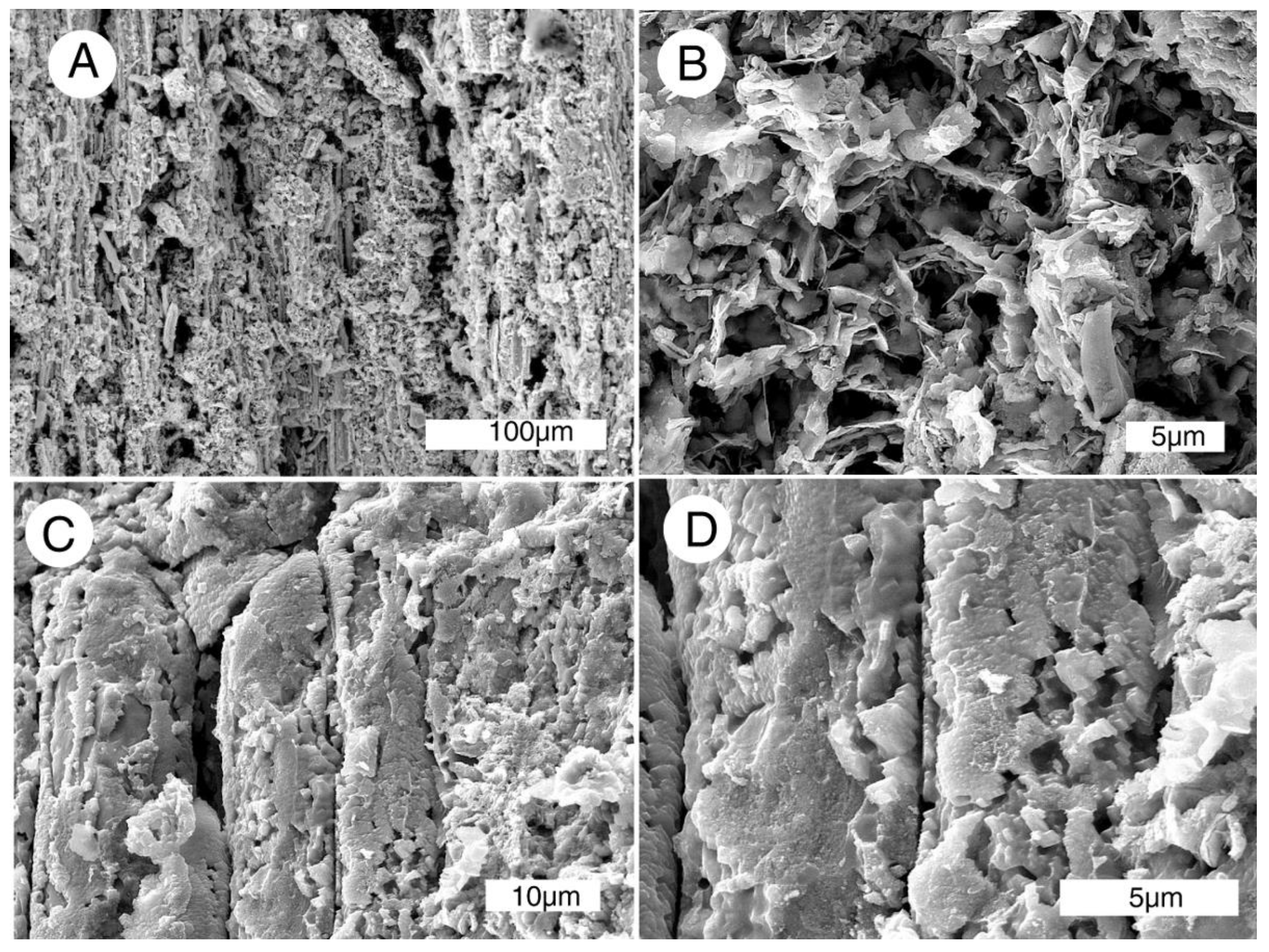
6. Manganese Oxide
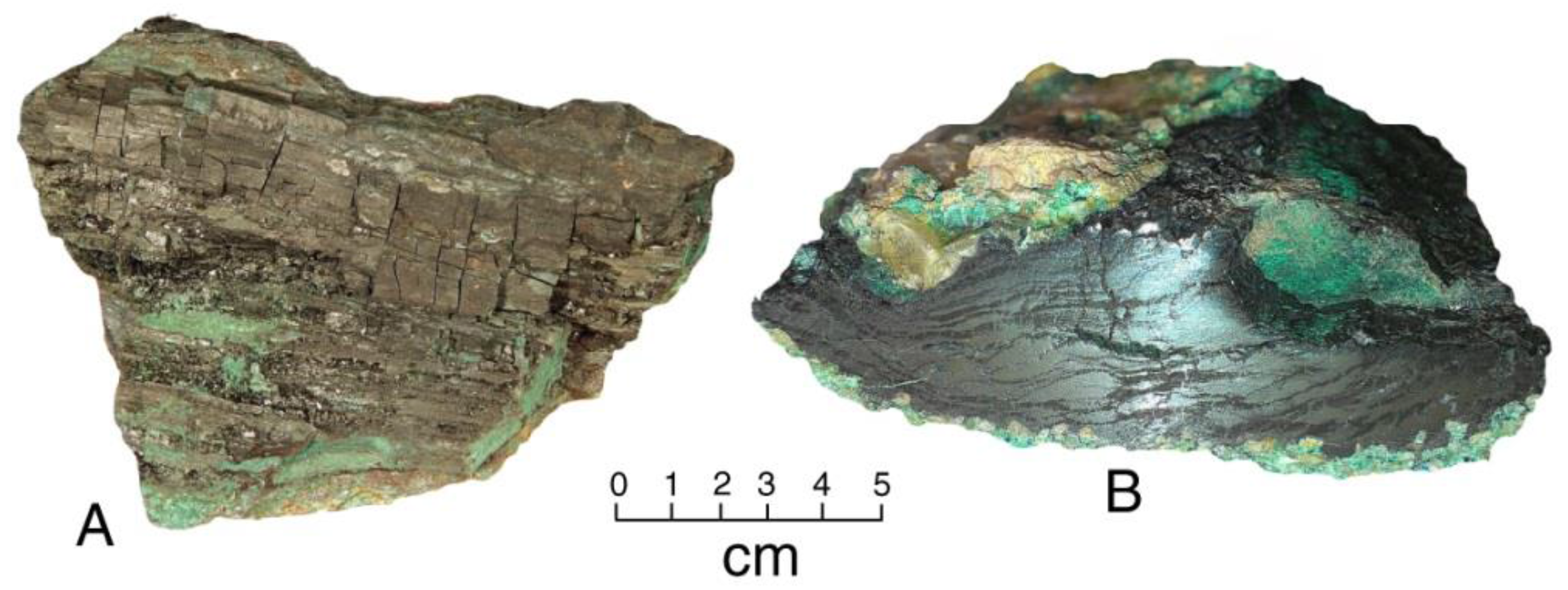
7. Copper Minerals
8. Fluorite
9. Barite
10. Volkonskoite: Chromian Smectite Clay
11. Natrolite and Calcite
12. Discussion
12.1. Calcite and Dolomite
12.2. Iron Minerals
12.3. Calcium Phosphate
12.4. Copper Minerals
12.5. Other Minerals
12.6. Highly-Localized Geochemical Conditions
12.7. Multiple Episodes of Mineralization
12.8. Possibilities for Future Research
Acknowledgments
Conflicts of Interest
References
- Mustoe, G.E. Wood petrifaction: A new view of permineralization and replacement. Geosciences 2017, 7, 119. [Google Scholar] [CrossRef]
- Buurman, P. Mineralization of fossil wood. Scr. Geol. 1972, 12, 1–43. [Google Scholar]
- Mustoe, G.E. Late Tertiary petrified wood from Nevada, USA: Evidence of multiple silicification pathways. Geosciences 2015, 5, 286–309. [Google Scholar] [CrossRef]
- Matysova, P.; Rössler, R.; Götze, J.; Leichmann, J.; Forbes, G.; Taylor, E.L.; Sakala, J.; Grygar, T. Alluvial and volcanic pathways to silicified plant stems (Upper Carboniferous-Triassic) and their taphonomic and paleoenvironmental meaning. Paleogeogr. Paleoclimatol. Paleoecol. 2010, 292, 127–143. [Google Scholar] [CrossRef]
- Siurek, J.; Chevallier, P.; Ro, C.; Chun, H.Y.; Youn, H.S.; Ziȩba, E.; Kuczumow, A. Studies on the wood tissue substitution by silica and calcite during preservation of fossil wood. J. Alloys Compd. 2004, 362, 107–115. [Google Scholar] [CrossRef]
- Greenland, C.W. The replacement of wood by calcite. Econ. Geol. 1918, 13, 116–119. [Google Scholar] [CrossRef]
- Galwitz, H. Verkalung undVerkisalung von Hőlzern in der Braunkhohle des Geiseltales. Wiss. Z. Univ. Halle, Math. Nat. 1954, 4, 41–44. [Google Scholar]
- Francis, J.E. Arctic Eden. Nat. Hist. 1991, 100, 57–62. [Google Scholar]
- Boyce, C.K.; Hazen, R.M.; Knoll, A.H. Nondestructive, in situ, cellular-scale mapping of elemental abundances in permineralized fossils. Proc. Nat. Acad. Sci. USA 2001, 98, 5970–5974. [Google Scholar] [CrossRef] [PubMed]
- Scott, A.C.; Collinson, M.E. Non-destructive multiple approaches to interpret the preservation of plant fossils: Implications for calcium-rich permineralizations. J. Geol. Soc. Lond. 2003, 160, 857–862. [Google Scholar] [CrossRef]
- Higgins, C.G. Calcification of some California Cretaceous wood. Geol. Soc. Am. Bull. 1960, 71, 1887–1888. [Google Scholar]
- Higgins, C.G. Significance of some fossil wood from California. Science 1961, 134, 473–479. [Google Scholar] [CrossRef] [PubMed]
- Lange, P.; Steiner, W. Rasterelektronenmikroskopische Untersuchungn an verkaltyen Holzresten aus dem plesitozaenen Travertin von Weimar. Quartaepalaeontologie 1984, 5, 225–236. [Google Scholar]
- Brand, L.S. Calcified wood found in Pleistocene sand. Ohio Acad. Sci. Proc. 1930, 8, 409. [Google Scholar]
- Brand, L.S. Calcified wood in upland sand near Cincinnati. Ohio J. Sci. 1932, 32, 55–62. [Google Scholar]
- Lorenz, V.J.; Röβler, R.; Schmitt, R.T. Fossiles Holz aus Fluorapatit und Calcit von der Tjörnes-Halbinsel, Nord-Island. Der Aufscluss 2010, 8, 17–25. [Google Scholar]
- Schwab, G. Über dolomitisiertes Holz aus der Weichbraunkohle von Malliss (Mecklenburg). Monatsber. Deutsch. Akad. Wiss. Berlin 1959, 1, 761–767. [Google Scholar]
- Vadász, E. Geological problems of fossil wood in Hungary. Acta Geol. Acad. Sci. Hung. 1964, 8, 119–143. [Google Scholar]
- Mustoe, G.E. Density and loss on ignition as indicators of the fossilization of silicified wood. IAWA J. 2016, 37, 98–111. [Google Scholar] [CrossRef]
- Bucovic, W.A. The Eocene Deltaic System of the Coal-Bearing Puget Group of Western Washington. In Cenozoic Paleogeography of the Western United States, Pacific Coast Paleogeography Symposium 3; Armentrout, J.M., Cole, M.R., TerBest, H., Eds.; The Pacific Section Society of Economic Paleontologists and Mineralogists: Los Angeles, CA, USA, 1979; pp. 147–163. [Google Scholar]
- Reolid, M.; Phillipe, M.; Nagy, J.; Abad, I. Preservation of phosphatic wood remains in marine deposits of the Brentskardhaugen Bed (Middle Jurassic) from Svalbard (Boreal Realm). Facies 2010, 56, 459–466. [Google Scholar] [CrossRef]
- Krajewski, K.P. Organic geochemistry of a phosphorite to black shale transgressive succession: Wilhelmøya and Janusfjellet Formations (Rhaetian-Jurassic) in Central Spitsbergen, Arctic Ocean. Chem. Geol. 1989, 74, 249–263. [Google Scholar] [CrossRef]
- Goldberg, E.D.; Parker, R.H. Phospatized wood from the Pacific sea floor. Geol. Soc. Am. Bull. 1960, 71, 631–632. [Google Scholar] [CrossRef]
- Arena, D.A. Exceptional preservation of plants and invertebrates by phosphatization, Riversleigh, Australia. Palaios 2008, 23, 495–502. [Google Scholar] [CrossRef]
- Glukoster, H.J.; Pierard, L.H.; Pfefferkorm, H.W. Apatite petrifactions in Pennsylvanian shales of Illinois. J. Sediment. Res. 1970, 40, 1363–1366. [Google Scholar]
- Jefferson, T.H. The preservation of conifer wood: Examples from the Lower Cretaceous of Antarctica. Paleontology 1987, 30, 233–249. [Google Scholar]
- Sweeney, I.J.; Chin, K.; Hower, J.C.; Budd, D.A.; Wolfe, D.G. Fossil wood from the middle Cretaceous Moreno Hill Formation: Unique expressions of wood mineralization and implications for the processes of wood preservation. Int. J. Coal Geol. 2009, 78, 1–17. [Google Scholar] [CrossRef]
- Viney, M.; Mustoe, G.E.; Dillhoff, T.A.; Link, P.S. The Bruneau Woodpile: A Miocene phosphatized wood locality in southwestern Idaho, USA. Geosciences 2017, 7, 82. [Google Scholar] [CrossRef]
- Pailler, D.; Flicoteaux, R.; Ambrosi, J.P.; Medus, J. The Mio-Pliocene fossil woods from Nkondo (Lake Albert, Uganda), mineral composition and formation. C. R. Acad. Bulgare Sci. Série II Fascicule A 2000, 331, 279–286. [Google Scholar]
- Koenigeur, J.C. Sur une liane plio-quatrinaire du Tchad. Bull. Mus. Natn. Hist. Nat. Sci. de la Terre 1973, 172, 81–91. [Google Scholar]
- Fleischer, M. Recent Estimates of the Abundances of Elements in the Earth’s Crust; U.S. Geological Survey Circular 285; USGS: Reston, VA, USA, 1953; pp. 1–3.
- Wedepohl, K.H. The composition of the continental crust. Geochim. Cosmochim. Acta 1995, 59, 1217–1232. [Google Scholar]
- Garcia-Guinea, J.; Martinez-Frias, J.; Harffy, M. Cell-hosted pyrite framboids in fossil woods. Naturwissenschaften 1988, 85, 78–81. [Google Scholar] [CrossRef]
- Tibbs, S.L.; Briggs, D.E.G.; Prossl, K.F. Pyritization of plant fossils from the Devonian Hunsrück Slate of Germany. Palaeontol. Z. 2003, 77, 241–246. [Google Scholar] [CrossRef]
- Briggs, D.E.G.; Raiswll, R.; Bottrell, S.H.; Hatfield, D.; Bartels, C. Controls on the pyriitization of exceptionally preserved fossils: An analysis of the Lower Devonian Hunstrück slate of Germany. Am. J. Sci. 1996, 296, 633–663. [Google Scholar] [CrossRef]
- Strullu-Derrien, C.; Kenrick, P.; Tafforeau, P.; Cochard, H.; Bonnemain, J.; Le Hérisse, A.; Lardeux, H.; Badel, E. The earliest wood and its hydraulic properties documented in c. 407-million-year-old fossils using synchroton microrotomography. Bot. J. Linnean Soc. 2014, 175, 423–437. [Google Scholar] [CrossRef]
- Kenrick, P.; Edwards, D. Anatomy of the Lower Devonian Gosslingia breconensis Heard based on pyritised axes with some comments on the permineralization process. Bot. J. Linnean Soc. 1988, 97, 95–123. [Google Scholar]
- Mustoe, G.E.; Viney, M. Mineralogy of Paleocene wood from Cherokee Ranch fossil forest, central Colorado, USA. Geosciences 2017, 7, 23. [Google Scholar] [CrossRef]
- Grimes, S.T.; Brock, F.; Rickard, D.; Davies, K.L.; Edwards, D.; Briggs, D.E.G.; Parkes, R.J. Understanding fossilization: Experimental pyritization of plants. Geology 2001, 29, 123–126. [Google Scholar] [CrossRef]
- Grimes, S.T.; Davies, K.L.; Butler, I.B.; Brock, F.; Edwards, D.; Rickard, D.; Briggs, D.E.G.; Parkes, R.J. Fossil plants from the Eocene London Clay: The use of pyrite textures to determine the mechanism of pyritization. J. Geol. Soc. 2002, 159, 493–501. [Google Scholar] [CrossRef]
- Roberts, L.B. Petrified wood composed of iron oxide. J. Geol. 1940, 48, 212–213. [Google Scholar] [CrossRef]
- Daber, R. Betrachtung über Markasitisierung eines Koniferenholzes aus dem Miozän der Tongrube von Guttau, Kries Bautzen. Geologie 1953, 2, 263–265. [Google Scholar]
- Martin-Penela, A.J.; Barregan, G. Silicification of plant remains in Messinian marine sediments in the Vera Basin (Almeria, Spain). Ecolgae Geol. Helv. 2003, 88, 557–593. [Google Scholar]
- Turner, J.P.; Saunders, J.A.; Cook, R.B. Petrographic evidence for amorphous silica precursors and geomicrobiologic processes in silicified and pyritized Holocene wood. In Proceedings of the Geological Society of America Annual Meeting, Denver, CO, USA, 27–30 October 2002; p. 493. [Google Scholar]
- Henstra, S.; Buurman, P.; Thiel, F. Investigation of fossilization processes in wood with the scanning electron microscope. JEOL News 1973, 10, 1–2. [Google Scholar]
- Scurfield, G. Wood petrifaction: An aspect of biomineralogy. Aust. J. Bot. 1979, 27, 377–390. [Google Scholar] [CrossRef]
- Nowak, J.; Florek, M.; Kwiatek, W.M.; Kuczumow, A. Composite structure of wood cells in petrified wood. Mater. Sci. Eng. C-Mater. Biol. Appl. 2007, 25, 119–130. [Google Scholar] [CrossRef]
- Hassan, K.M. The iron mineralogy of Eocene fossil wood—A Mőssbauer study of samples from the petrified forest, New Cairo, Egypt. Can. Mineral. 2015, 53, 705–716. [Google Scholar] [CrossRef]
- Schellenberg, S.A. Mazon Creek: Preservation in late Paleozoic deltaic and marginal marine environments. In Exceptional Fossil Preservation: A Unique View on the Evolution of Marine Life; Etter, W., Hagadorn, J.W., Tang, C.M., Bottjer, D.J., Eds.; Columbia University Press: New York, NY, USA, 2002; pp. 185–203. [Google Scholar]
- Williams, C.J.; Trostle, K.D.; Sunderlin, D. Fossil wood in coal-forming environments of the Late Paleocene–Early Eocene Chickaloon Formation. Paleogeogr. Paleoclimatol. Paleoecol. 2010, 295, 363–375. [Google Scholar] [CrossRef]
- Reinink-Smith, L.; Leopold, E.B. Warm climate in the Late Miocene of the south coast of Alaska and the occurrence of Podocarpaceae pollen. Palynology 2005, 29, 205–262. [Google Scholar] [CrossRef]
- Hayes, J.B.; Harms, J.C.; Wilson, T., Jr. Contrasts between braided and meandering stream deposits, Beluga and Sterling Formations (Tertiary), Cook Inlet, Alaska. In Recent and Ancient Sedimentary Environments in Alaska, Proceedings of the Alaska Geological Society Symposium, Anchorage, AL, USA, 2–4 April 1975; Miller, T.P., Ed.; Alaska Geological Society: Anchorage, AL, USA, 1976; pp. J1–J27. [Google Scholar]
- Polgári, M.; Phillipe, M.; Szabo-Drubina, M.; Tóth, M. Manganese-impregnated wood from a Toarcian manganese deposit, Eplény Mine, Bakony Mtns., Hungary. N. Jb. Geol. Paläont. Mh. 2005, 200, 175–192. [Google Scholar]
- Scurfield, G.; Segnit, E.R. Petrifaction of wood by silica minerals. Sediment. Geol. 1984, 39, 149–167. [Google Scholar] [CrossRef]
- Leo, R.F.; Barghoorn, E.S. Silicification of Wood. Bot. Mus. Lealf. Harv. Univ. 1976, 25, 1–47. [Google Scholar]
- Talbott, L.W. Nacimiento Pit, A Triassic Strata-Bound Copper Deposit. In Ghost Ranch, New Mexico Geological Society Guidebook 25; Siemens, C.T., Woodward, L.A., Callender, L.A., Eds.; New Mexico Geological Society: Socorro, NM, USA, 1974; pp. 301–303. [Google Scholar]
- Woodward, L.A.; Kaufman, W.H.; Schumacher, D.L. Sandstone copper deposits. In Ghost Ranch, New Mexico Geological Society Guidebook 25; Siemens, C.T., Woodward, L.A., Callender, L.A., Eds.; New Mexico Geological Society: Socorro, NM, USA; pp. 295–299.
- Woodward, L.A.; Kaufman, W.H.; Schumacher, D.L. Strata-bound copper deposits in Triassic sandstone of Sierra Nacimiento. N. M. Econ. Geol. 1974, 69, 108–120. [Google Scholar] [CrossRef]
- Woodward, L.A. Geology and Mineral Resources of Sierra Nacimiento and vicinity, New Mexico. New Mexico Bureau of Mines and Mineral Resources: Socorro, NM, USA; 1987; 84p. [Google Scholar]
- Cowart, J.B.; Milne, J.J. Remediation of 25 million gallons of acidic groundwater, Nacimiento Copper Mine site, Cuba, New Mexico. In Proceedings of the 11th Tailings and Mine Wastes Conference, Vail, CO, USA, 10–13 October 2004; pp. 167–172. [Google Scholar]
- Suneson, N.H. Petrified wood in Oklahoma, Oklahoma Geological Survey Information Series 14, Norman, Oklahoma, USA. 2010, p. 19. Available online: http://www.ogs.ou.edu/geology/pdf/PetWoodIS_14,pdf.pdf (accessed on 21 December 2017).
- Fay, O. Bibliography of Copper Occurrences in Pennsylvanian and Permian Red Beds and Associated Rocks in Oklahoma, Texas, and Kansas (1805–1996); Oklahoma Geological Survey Special Publication 2000-1; Oklahoma Geological Survey: Norman, Oklahoma, 2000; p. 16. [Google Scholar]
- Gönder, Y. Zile opalized cola wood. Veni Tokat, 30 August 2014; 5. (In Turkish) [Google Scholar]
- Akkemik, U.; Türkoğlu, N.; Poole, I.; Çiçek, I.; Köse, N.; Gürgen, G. Woods of a Miocene petrified forest near Ankara, Turkey. Turk. J. Agric. For. 2008, 33, 89–97. [Google Scholar]
- Witke, K.; Götze, J.; Röβler, R.; Dietrich, D.; Marx, G. Raman and cathodoluminescence spectroscopic investigation on Permian fossil wood from Chemnitz—a contribution to the study of the permineralization process. Spectrochem. Acta Part A 2004, 60, 2903–2913. [Google Scholar] [CrossRef] [PubMed]
- Röβler, R. Two remarkable Permian petrified forests: Correlation, comparison, and significance. In Non-Marine Permian Biostratigraphy and Biochronology; Lucas, S.G., Cassinis, G., Schneider, J.W., Eds.; Special Publications: London, UK, 2006; Volume 265, pp. 48–53. [Google Scholar]
- Röβler, R.; Annacker, V.; Kretzschmar, R.; Eulenberger, S.; Tunger, B. Auf Schatzsuche in Chemnitz—Wissenschaftliche Grabungen ’08. Veröffentlichungen Museum Naturkunde 2008, 31, 5–44. [Google Scholar]
- Läbe, S.; Gee, C.T.; Ballhaus, C.; Nagel, T. Experimental silicification of the tree fern Dicksonia antarctica at high temperature with silica-enriched H2O vapor. Palaios 2012, 27, 835–841. [Google Scholar] [CrossRef]
- Luthardt, L.; Röβler, R.; Schneider, J.W. Palaeoclimatic and site-specific conditions in early Permian fossil forest of Chemnitz—Sedimentological, geochemical and palaeobotanical evidence. Palaeogeogr. Palaeoclimatol. Palaeoecol. 2016, 441, 627–652. [Google Scholar] [CrossRef]
- Schmidt, E. Unbekannte Fundstellen rund um Sobernheim/Nahe. Aufschluß 1979, 11, 383–388. [Google Scholar]
- Winckler, K.M. “Hülsenfrüchte” aus dem Oligozän—Die Grube Steinhardt bei Sobernheim. Fossilien 1984, 6, 253–257. [Google Scholar]
- McConnell, D. An American occurrence of volkonskoite. Clays Clay Miner. 1953, 2, 152–155. [Google Scholar] [CrossRef]
- Foord, E.E.; Starkey, H.C.; Taggart, J.E.; Swawe, D.R. A reassessment of the volkonskoite-chromian smectite nomenclature problem. Clays Clay Miner. 1987, 35, 139–149. [Google Scholar] [CrossRef]
- Oldman, O.H. Volcanic rocks of Mount Elgon in British East Africa. Geol. Fören. Förhandl. 1930, 455–537. [Google Scholar] [CrossRef]
- Kräusel, E.; Frankfurt, A.M. Das Alter der fossilen Hölzer vom Mt. Elgon, Brit. Ost-Africa. GIF 1934, 56, 489–492. [Google Scholar]
- Bancroft, H. Some fossil dicotyledonous woods from Mount Elgon, East Africa I. Am. J. Bot. 1935, 22, 164–183. [Google Scholar] [CrossRef]
- Bancroft, H. Some fossil dicotyledonous woods from Mount Elgon, East Africa II. Am. J. Bot. 1935, 22, 279–290. [Google Scholar] [CrossRef]
- Bancroft, H. The Stockholm collections of fossil woods from Mount Elgon: Supplementary note. GFF 1936, 58, 393–396. [Google Scholar] [CrossRef]
- Bloomfield, K. Carbonatite-derived sediments in southeast Uganda. J. Geol. Soc. Lond. 1972, 128, 507–511. [Google Scholar] [CrossRef]
- Davies, K.A. The building of Mount Elon (East Africa). In Geological Survey of Uganda Memoir VII; Benham and Company: Colchester, UK, 1952; 72p. [Google Scholar]
- Utami, W.S.; Herdianita, N.R.; Atmaja, R.W. The Effect of Temperature and pH on the Formation of Silica Scaling of Dieng Geothermal Field, Central Java, Indonesia. In Proceedings of the Thirty-Ninth Workshop on Geothermal Reservoir Engineering Stanford University, Stanford, CA, USA, 24–26 February 2014. [Google Scholar]
- Nicholson, K. Geothermal Fluids: Chemistry and Exploration Techniques; Springer: Berlin, Germany, 1968; 263p. [Google Scholar]
- Hardie, L.A. Dolomotization, a critical view of some current views. J. Sediment. Res. 1987, 57, 166–183. [Google Scholar] [CrossRef]
- Henderson, G.S.; Black, P.M.; Rodgers, K.A.; Rankin, P.C. New data on New Zealand viviantite and metavivianite. N. Z. J. Geol. Geophys. 1984, 27, 367–378. [Google Scholar]
- Hem, J.D. Reaction of metal ions at surfaces of hydrous iron oxides. Geochim. Cosmochim. Acta 1977, 41, 527–538. [Google Scholar] [CrossRef]
- Lemos, V.P.; Lima da Costa, M.; Lemos, R.I.; Gomes de Faria, M.S. Vivianite and siderite in lateritic iron crust: An example of bioreduction. Quim. Nova 2007, 30, 36–40. [Google Scholar] [CrossRef]
- McKelvey, V.E. Phosphate Deposits. In U.S. Geological Survey Bulletin 125-D; U.S. Government Publishing Office: Washington, DC, USA, 1967; 21p. [Google Scholar]
- Chow, L.C. Solubility of Calcium Phosphates. In Octacalcium Phosphate; Chow, L.C., Eanes, E.D., Eds.; Karger: Basel, Switzerland, 2001; Volume 18, pp. 94–111. Available online: http://www.bio.umass.edu/biology/kunkel/pub/lobster/PDFs/CrystalChemistry/Chow&Eanes_SolCaP-MOrSci2001.pdf (accessed on 21 December 2017).
- Mustoe, G.E. Mineralogy and geochemistry of late Eocene silicified wood from Florissant Fossil Beds National Monument, Colorado. In Paleontology of the Upper Eocene Florissant Formation, Colorado; Meyer, H.W., Smith, D.M., Eds.; Geological Society of America Special Paper 35; Geological Society of America: Boulder, CO, USA, 2008; pp. 127–140. [Google Scholar]
- Viney, M.; Dietrich, D.; Mustoe, G.E.; Link, P.; Lampke, T.; Götze, J.; Röβler, R. Multi-stage silicification of Pliocene wood: Re-examination of a 1985 discovery from Idaho, USA. Geosciences 2016, 6, 21. [Google Scholar] [CrossRef]
- Root, J.V. Bruneau wood. Gems Miner. 1971, 409, 36–37. [Google Scholar]


| Mineralization | Age | Location | Reference |
|---|---|---|---|
| Calcite | Jurassic | Lucków, Poland | [5] |
| Calcite | Cretaceous | Isle of Wight, England | [2] |
| Calcite | Cretaceous | Kansas, USA | [6] |
| Calcite | Eocene | Geiseltal, Germany | [7] |
| Calcite | Eocene | British Columbia, Canada | This report |
| Calcite | Eocene | Ellesmere Island Arctic Canada | [8] |
| Calcite | Miocene | Washington, USA | [9] |
| Calcite | Neogene | Florida, USA | [1] |
| Calcite | Pliocene | Dunrobba, Italy | [10] |
| Calcite | Pleistocene | California, USA | [11,12] |
| Calcite | Pleistocene | Weimar, Germany | [13] |
| Calcite | Pleistocene | California, USA | [14,15] |
| Calcite | Pleistocene | Northern Iceland | [16] |
| Dolomite | unknown | Germany | [17] |
| Dolomite | unknown | Hungary | [18] |
| Dolomite | Eocene | Washington, USA | This report |
| Issaquah | ||
|---|---|---|
| Oxide | Weight % | Atomic % |
| MgO | 32.6 | 41.2 |
| Al2O3 | 4.8 | 2.4 |
| SiO2 | 5.3 | 4.5 |
| CaO | 55.7 | 51.9 |
| Fe2O3 * | 0 | 0 |
| Black Diamond Coal Mine | ||
| MgO | 29.8 | 38.1 |
| Al2O3 | 0.74 | 0.38 |
| SiO2 | 3.6 | 3.1 |
| CaO | 56.3 | 51.7 |
| Fe2O3 * | 0.52 | 6.8 |
| Location | Age | Setting | Reference |
|---|---|---|---|
| Foy, France | Carboniferous | Continental | [2] |
| Illinois, USA | Jurassic | Continental | [25] |
| Svalbard, Boreal Realm | Jurassic | Marine | [21,22] |
| Swindon, England | Jurassic | Marine | [10] |
| Antarctica | Cretaceous | Continental | [26] |
| Winterswijk, Netherlands | Cretaceous | Continental | [2] |
| New Mexico, USA | Cretaceous | Continental | [27] |
| California, USA | Eocene | Continental | [28] |
| Australia | Miocene/Oligocene | Continental | [23] |
| Nevada, USA | Miocene | Continental | [28] |
| Idaho, USA | Miocene | Continental | [28] |
| Mt. Elgon, Uganda | Miocene/Pliocene | Continental | [29] |
| Florida, USA | Neogene | Continental | [28] |
| Republic of Chad | Pliocene/Pleistocene | Continental | [30] |
| Northern Iceland | Pleistocene | Continental | [16] |
| Pacific sea floor | Holocene | Marine | [23] |
| Mineralization | Age | Location | Reference |
|---|---|---|---|
| Pyrite | Permian | Guadalajara, Spain | [33] |
| Pyrite | Devonian | Hunsrück, Germany | [34,35] |
| Pyrite | Devonian | Western France | [36,37] |
| Pyrite | Paleocene | Colorado, USA | [38] |
| Pyrite | Eocene | California, USA | This report |
| Pyrite | Eocene | Kent, England | [39,40] |
| Pyrite | Eocene | Louisiana, USA | [41] |
| Marcasite | Miocene | Dresden, Germany | [42] |
| Pyrite | Pliocene | Alméria, Spain | [43] |
| Pyrite | Holocene | Georgia, USA | [44] |
| Pyrite & Hematite | Cretaceous | Hautrage, Belgium | [2] |
| Iron oxide | Cretaceous | Oklahoma, USA | This report |
| Iron oxide | Cretaceous | Montana, USA | This report |
| Iron oxide | Pliocene | California, USA | This report |
| Iron oxide | Quaternary | Siberia, USSR | [2] |
| Goethite | unknown | unknown | [45] |
| Goethite | unknown | Australia | [46] |
| Goethite | Jurassic | Luków, Poland | [47] |
| Goetite | Permian | Saiwan, Oman | [4] |
| Goethite | Eocene | British Columbia, Canada | This report |
| Goethite & Hematite | Eocene | Cairo, Egypt | [48] |
| Goethite & Hematite | Pliocene | Dunrobba, Italy | [47] |
| Goethite & Lepidocrocite | Oligocene | Düsseldorf, Germany | [2] |
| Goethite & Lepidocrocite | Pleistocene | Ugchelen, The Netherlands | [2] |
| Siderite | unknown | Siegen, Germany | [2] |
| Siderite | unknown | Australia | [2] |
| Siderite | Pennsylvanian | Illinois & Indiana, USA | [49,50] |
| Siderite | Paleocene | Alaska, USA | [51] |
| Siderite | Paleogene | Alaska, USA | [52] |
| Siderite | Neogene | Alaska, USA | [53] |
| Siderite & Hematite | unknown | Niederpleis, Germany | [2] |
| Siderite & Pyrite | Pleistocene | Oosterbeck, The Netherlands | [2] |
| Hollandite & limonite * | Jurassic | Transnubia, Hungary | [53] |
| Mn-Fe oxide | Miocene | Nevada, USA | This report |
| Analysis 1 | Analysis 2 | Mean | ||||
|---|---|---|---|---|---|---|
| Element | Weight % | Atomic % | Weight % | Atomic % | Weight % | Atomic % |
| Si | 1.9 | 2.5 | 2.4 | 2.9 | 2.2 | 2.7 |
| Ca | 1.7 | 1.5 | 1.7 | 1.5 | 1.7 | 1.5 |
| Mn | 45.9 | 23.3 | 40.4 | 25.1 | 43.2 | 25.2 |
| Fe | 25.0 | 15.1 | 31.3 | 19.1 | 28.2 | 17.1 |
| O | 24.4 | 51.6 | 24.2 | 51.5 | 24.3 | 51.5 |
| Element | Analysis 1 | Analysis 2 | Analysis 3 | Average | ||||
|---|---|---|---|---|---|---|---|---|
| Weight % | Atomic % | Weight % | Atomic % | Weight % | Atomic % | Weight % | Atomic % | |
| O | 20.4 | 48.1 | 20.9 | 48.7 | 27.2 | 55.6 | 22.8 | 50.8 |
| Al | 0.20 | 0.28 | 0.34 | 0.47 | 0.64 | 0.78 | 0.39 | 0.51 |
| Si | 0.82 | 1.09 | 1.07 | 1.42 | 3.61 | 4.21 | 2.11 | 2.24 |
| As | 1.13 | 0.57 | 1.12 | 0.56 | 1.39 | 0.61 | 1.21 | 0.58 |
| Ti | 2.03 | 1.59 | 1.96 | 1.53 | 8.48 | 5.80 | 4.16 | 2.97 |
| Fe | 2.90 | 1.95 | 2.06 | 1.37 | 0.93 | 0.54 | 1.96 | 1.29 |
| Cu | 48.8 | 29.9 | 49.3 | 28.3 | 37.0 | 19.1 | 45.0 | 25.8 |
| V | 23.7 | 17.5 | 24.2 | 17.7 | 20.8 | 13.4 | 22.9 | 18.4 |
| Cu:V | 3.4:2 | 3.2:2 | 2.8:2 | 2.8:2 | ||||
© 2018 by the author. Licensee MDPI, Basel, Switzerland. This article is an open access article distributed under the terms and conditions of the Creative Commons Attribution (CC BY) license (http://creativecommons.org/licenses/by/4.0/).
Share and Cite
Mustoe, G.E. Mineralogy of Non-Silicified Fossil Wood. Geosciences 2018, 8, 85. https://doi.org/10.3390/geosciences8030085
Mustoe GE. Mineralogy of Non-Silicified Fossil Wood. Geosciences. 2018; 8(3):85. https://doi.org/10.3390/geosciences8030085
Chicago/Turabian StyleMustoe, George E. 2018. "Mineralogy of Non-Silicified Fossil Wood" Geosciences 8, no. 3: 85. https://doi.org/10.3390/geosciences8030085
APA StyleMustoe, G. E. (2018). Mineralogy of Non-Silicified Fossil Wood. Geosciences, 8(3), 85. https://doi.org/10.3390/geosciences8030085