Investigation of Preprocessing for Seismic Attenuation Profiling to Image the Earthquake Swarm Associated with the 2000 Eruption of the Miyakejima Volcano in Japan

Abstract

By using profiling that focuses on seismic attenuation instead of reflectivity, we investigate geological structures in volcanic areas and fractured areas, where seismic reflections are difficult to observe. A previous study successfully visualized the hypocenter distribution of the earthquake swarm associated with the 2000 Miyakejima eruption from the seismic attenuation profile of a seismic line. However, any significant geologic features were not figured out on other nearby lines. In this paper, we re-evaluated our preprocessing of the seismic reflection data, which are the input for the seismic attenuation profiling method, with an eye toward improving frequency preservation. First, deconvolution was excluded from the preprocessing sequence, because it can potentially change the frequency content of seismic data. Second, a very small NMO stretching factor of 0.1, which does not allow reflections to stretch more than 10%, was adopted to minimize the frequency distortion by NMO correction. As a result, clear high-attenuation anomalies showed up on seismic attenuation profiles of the other nearby lines, which are consistent with typical geological features known in the study area: earthquake swarm and volcanic activity. This paper demonstrates that appropriate preprocessing was able to improve the accuracy of imaging geological structures by seismic attenuation profiling.

1. Introduction

Seismic reflection profiles are widely used in oil and gas exploration, and studies of crustal structure, because they enable researchers to visualize sedimentary structures on the basis of reflection continuity and faults on the basis of offset reflections. However, the reflection profiles are unable to be utilized in poorly reflective areas, such as volcanic areas or highly fractured regions, where seismic reflections are inherently difficult to observe.

Only a few techniques have been tested to overcome this limitation, most notably seismic attribute analysis [1] and seismic scattering analysis [2]. These methods focus on seismic attributes other than reflection amplitude to successfully extract subsurface geological information. 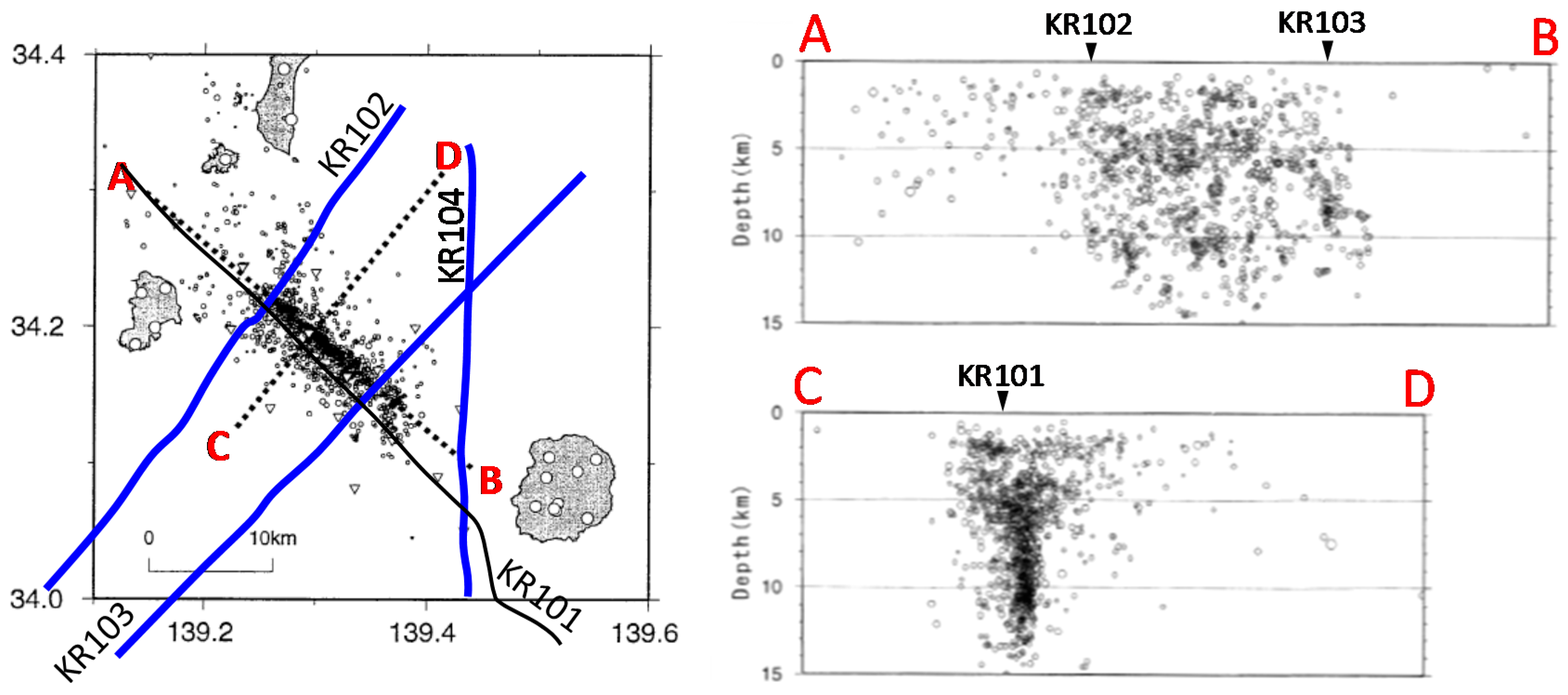From the same point of view, we applied seismic attribute analysis based on the attenuation property called ‘seismic attenuation profiling’ (SAP) in a previous study [3]. This study looked at the volcanic area between the Miyakejima, Kozushima, and Niijima island volcanos in Japan (Figure 1). It discerned a remarkable, down-warping, high-attenuation anomaly on a seismic survey line (KR101) between Miyakejima and Kozushima islands, which was well-correlated with the hypocenter distribution of the earthquake swarm associated with the 2000 eruption of Miyakejima Volcano (Figure 2). However, no significant geological features have been observed on the other seismic lines (KR102, KR103, and KR104). Specifically, the signal-to-noise (S/N) ratio and the frequency distortion of seismic reflection data to be input to SAP analysis remains an obstacle in expanding SAP method to a regional study and to spatial or 3D applications. To address this problem, this study is a re-examination of the preprocessing of the seismic reflection data that were used in the previous SAP study [3].

2. Methods

The SAP method is a technique for imaging seismic attenuation structures from seismic reflection data [3]. The method can be used for geophysical imaging in poorly reflective areas such as volcanic or highly-faulted regions, because it does not require continuous reflections. However, the current SAP method, which uses the spectral ratio, has a disadvantage in that it is dependent on the quality of the input seismic reflection data. It is particularly reliant on effective frequency preservation during data preprocessing, such as normal moveout (NMO) correction and deconvolution.

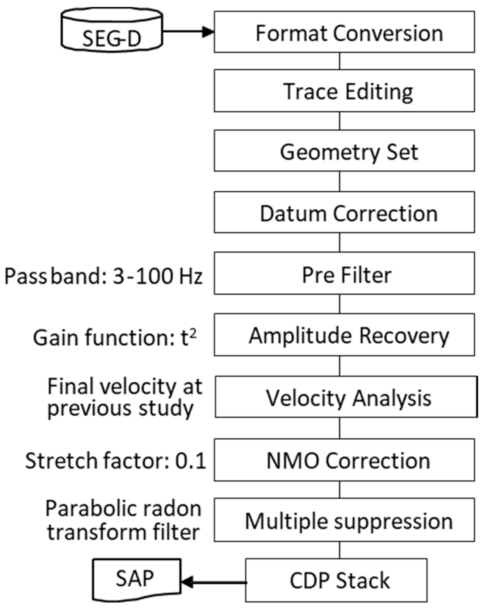
Previously, we used poststack seismic data because of high S/N ratio [3], whereas prestack data was used in another previous study [6] to avoid frequency distortion by NMO correction. However, neither study addressed deconvolution effect in frequency content preservation; thus, we excluded deconvolution from the preprocessing sequence in the present study. Thereafter, to reduce the effects of frequency distortion caused by NMO correction, a very small NMO stretching factor of 0.1 (10%) was adopted. The preprocessing flow chart used in this study is shown in Figure 3.

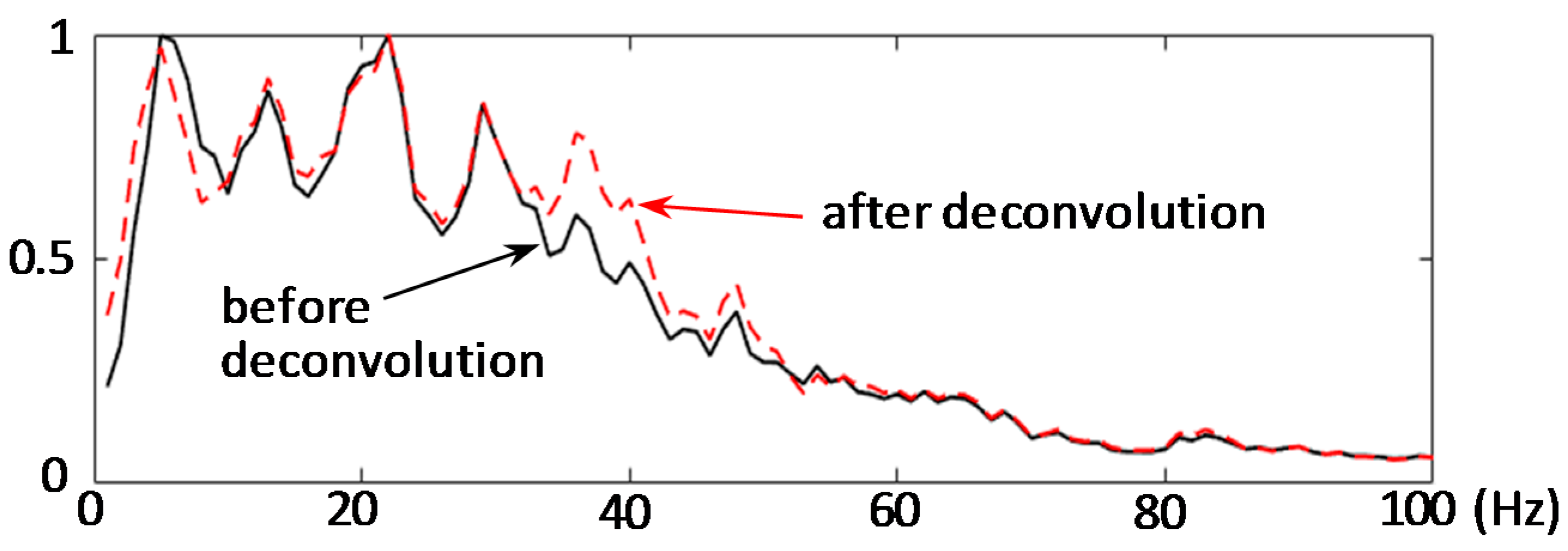
Figure 4 shows an example of frequency distortion by deconvolution. Spectrums before and after the deconvolution are compared in this figure. As seen in the figure, the relatively high frequency components of 30–50 Hz are raised by the deconvolution. Therefore, it is better to exclude the deconvolution from the preprocessing sequence.

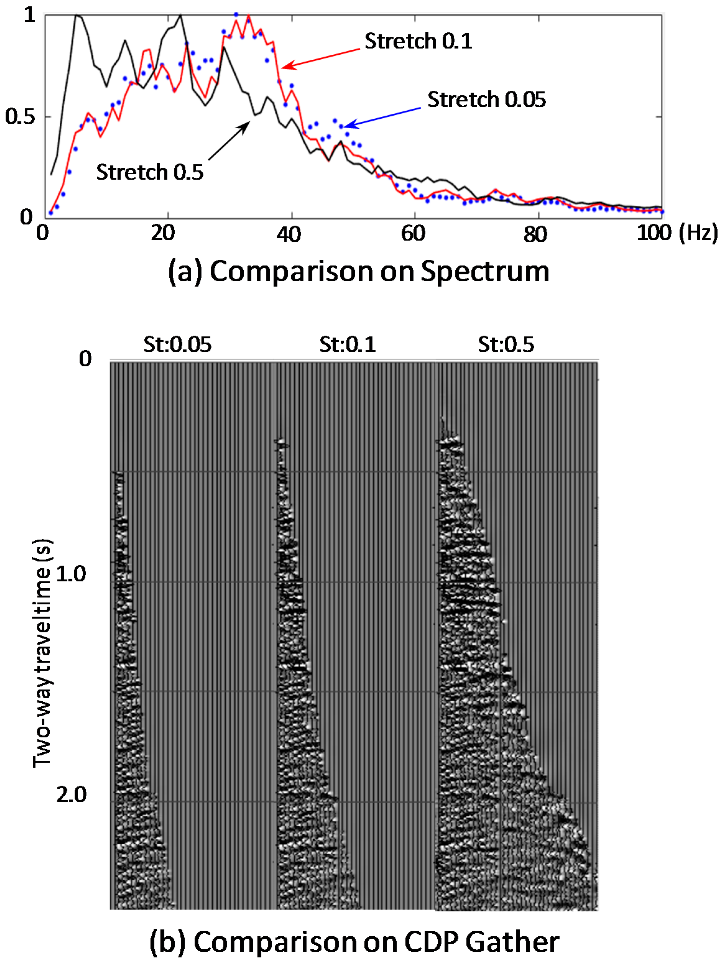
Figure 5 is an example of frequency distortion by NMO stretch factor. The top figure shows difference in spectrums by NMO stretch factors: 0.5, 0.1, and 0.05. Both frequency contents from the stretch factors 0.1 and 0.05 are nearly consistent. However, the frequency content from the stretch factor 0.5 is significantly different from the others. Those results indicate that we should use the stretch factor of 0.1 for the seismic reflection data presently used. The bottom figure shows CDP gathers after NMO correction with every stretch factor. We can also see that both CDP gathers by the NMO correction with stretch factors 0.1 and 0.05 are nearly consistent.

For this study, we assumed that Q is constant over the seismic frequency band, as many previous authors did [7], although Q is frequency-dependent [8]. We calculated the average Q value by using the spectral ratio method, which is a general method for Q estimation [9,10]. The temporal decay in the amplitude of a propagating seismic wave of frequency f from traveltime t1 to traveltime t2 is written as a function of Q:

$$A_{t2}(f)=GR{A}_{t1}(f)\exp \left[-\frac{\pi f\delta t}{Q}\right],$$

(1)

in which δt = t2 − t1; A_t1 and A_t2 are the amplitude spectra of the wavelet at t1 and t2, respectively; and G and R are the geometrical spreading and reflection coefficients, respectively. Taking the spectral ratio and then the logarithms of both sides yield:

$$\ln \left[\frac{A_{t2}(f)}{A_{t1}(f)}\right]=-\frac{\pi f\delta t}{Q}+\ln (GR)=pf+\ln (GR),$$

(2)

$$\mathrm{where},p=-\frac{\pi \delta t}{Q}.$$

(3)

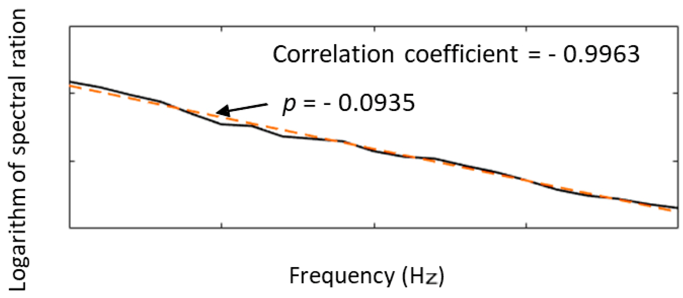
Given that the logarithm of the spectral ratio is a linear function of frequency f, as expressed in Equation (2), Q can be computed from its gradient p by using Equation (3) for the time window between t1 and t2.

As shown in Figure 6, we computed the gradient p by linear approximation with the least squares method. To evaluate the reliability of the Q estimation by the spectral ratio method, the correlation coefficients of the linear approximation were calculated at every location.

3. Results

3.1. Study Area and Data Specifications

Our study area is located near Miyakejima and Kozushima volcanic islands, approximately 170 km south of Tokyo, Japan (Figure 1). These volcanic islands are part of the Izu Islands, where volcanic activities accompanied by earthquake swarms have occurred repeatedly in recorded history [11]. On 26 June 2000, small volcanic earthquakes began to be recorded at observation stations west of the summit of the Miyakejima Volcano, and an earthquake swarm ensued [4]. The swarm migrated northwestward in the direction of Kozushima and Niijima and then developed into the most intense earthquake swarm ever observed near the Japanese archipelago [12] (Figure 2). The main eruption of the Miyakejima Volcano occurred at the summit on 8 July 2000 [11]. A number of earthquakes occurred during the two-month period following the eruption [13]. The hypocenter depths of the 2000 swarm activity between Miyakejima and Kozushima have been reported by several studies [11,12,13].

The seismic reflection data used in this study were obtained during the KR00-08 Cruise of R/V Kairei, which was conducted by Japan Agency for Marine-Earth Science and Technology (JAMSTEC) from 21 to 27 November 2000, five months after the swam beginning [3]. A total of 250 km of seismic reflection data were collected in the study area (Figure 1). Data acquisition was conducted using eight 25-L airguns with shot spacing of 50 m and a 156-channel streamer cable with a group interval of 25 m. The maximum offset length was 4.1 km [3].

The streamer cable was towed 20 m below the sea surface to avoid the effects of sea-wave noise generated by seasonal winds that were blowing during the whole survey period. Data preprocessing was carried out by careful trace editing; NMO correction with 0.1 stretching factor; multiple suppression; CDP stacking. Stratified layer with continuous reflections can be observed in the shallowest part of every seismic profile (Figure 7a, Figure 8a and Figure 9a) and almost energy of multiples appears to be suppressed below the stratified layer. These processing results indicate that the preprocessing was successful. However, strong ‘migration smile’ noises arose in the resulting migrated sections, because of possible diffractions coming from the sidewalls of nearby volcanic islands. Therefore, we adopted CDP stack records as the input data for the present SAP analysis.

3.2. Seismic Attenuation Profiles

Figure 7a–c shows the CDP stack section, correlation coefficient section, and seismic attenuation profile of average Q on KR102, respectively. Almost all of the correlation coefficients represent highly negative correlations (less than −0.8), thus indicating very good linear approximations in the gradient p determination. As shown in Figure 7c, a vertical high-attenuation anomaly was clearly observed around the intersection with KR101. Such anomaly was not imaged on KR102 in the previous study [3].

Figure 8 and Figure 9 show CDP stack sections, correlation coefficient sections, and average Q profiles of KR103 and KR104, respectively. As shown in Figure 8c, an up-warping high-attenuation anomaly can be observed on the average Q profile on KR103. This anomaly is located on the topographic high of the bathymetry (Figure 1). Furthermore, another up-warping high-attenuation anomaly can be observed in Figure 9c, the location of which is near the Miyakejima volcanic island.

4. Discussion

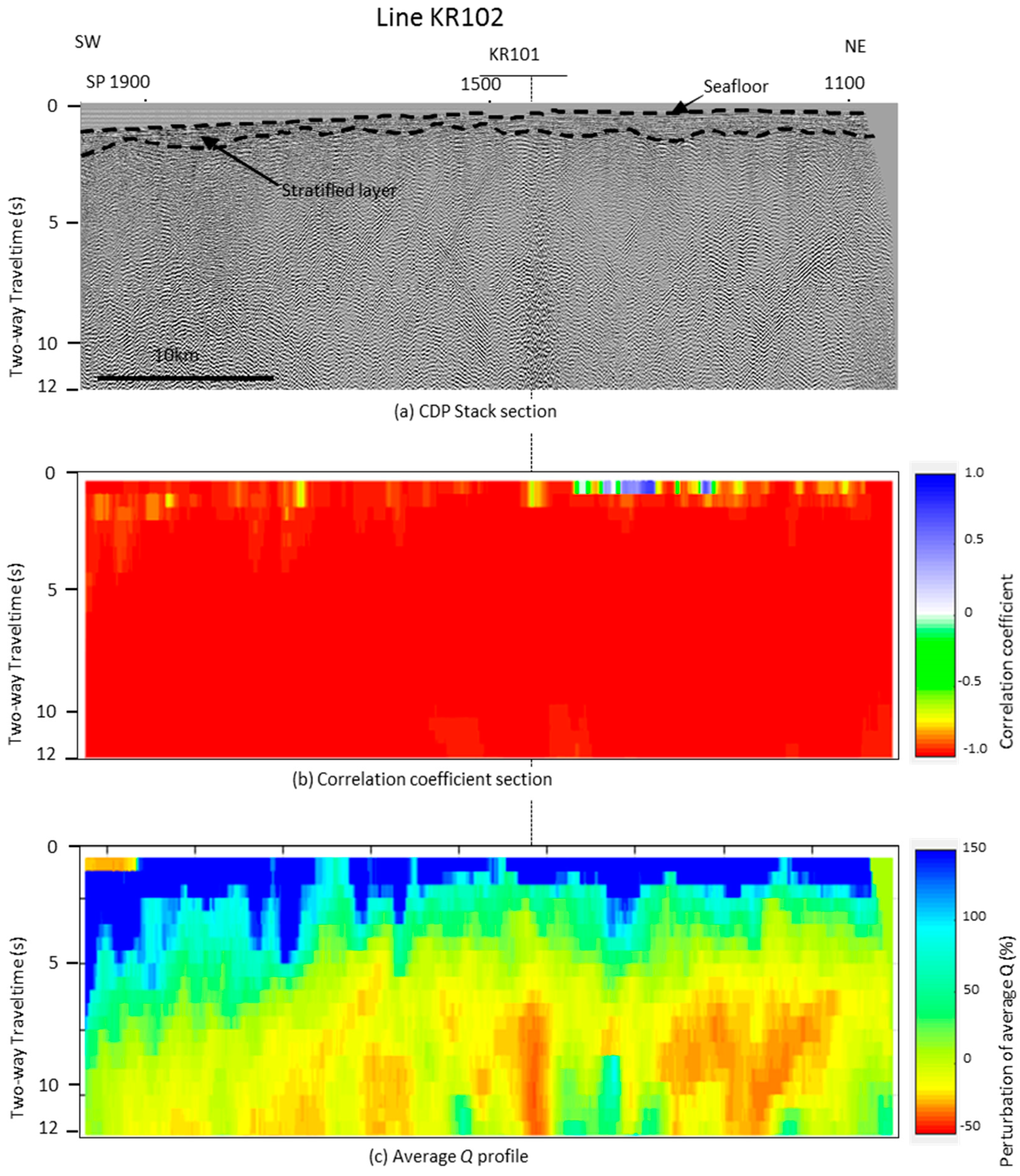
Several new attenuation anomalies were identified from the seismic attenuation profiles. They all were not imaged in the previous study [3]. Regarding the vertical high-attenuation anomaly observed on KR102 (Figure 7c), its shape is very similar to that of the cross section of the 2000 earthquake swarm shown in Figure 2. Additionally, its location is consistent with that of the swarm. Considering these similarityies in shape and location, it can be concluded that the vertical high-attenuation anomaly reflects the cross section of the hypocenter distribution of the 2000 swarm.

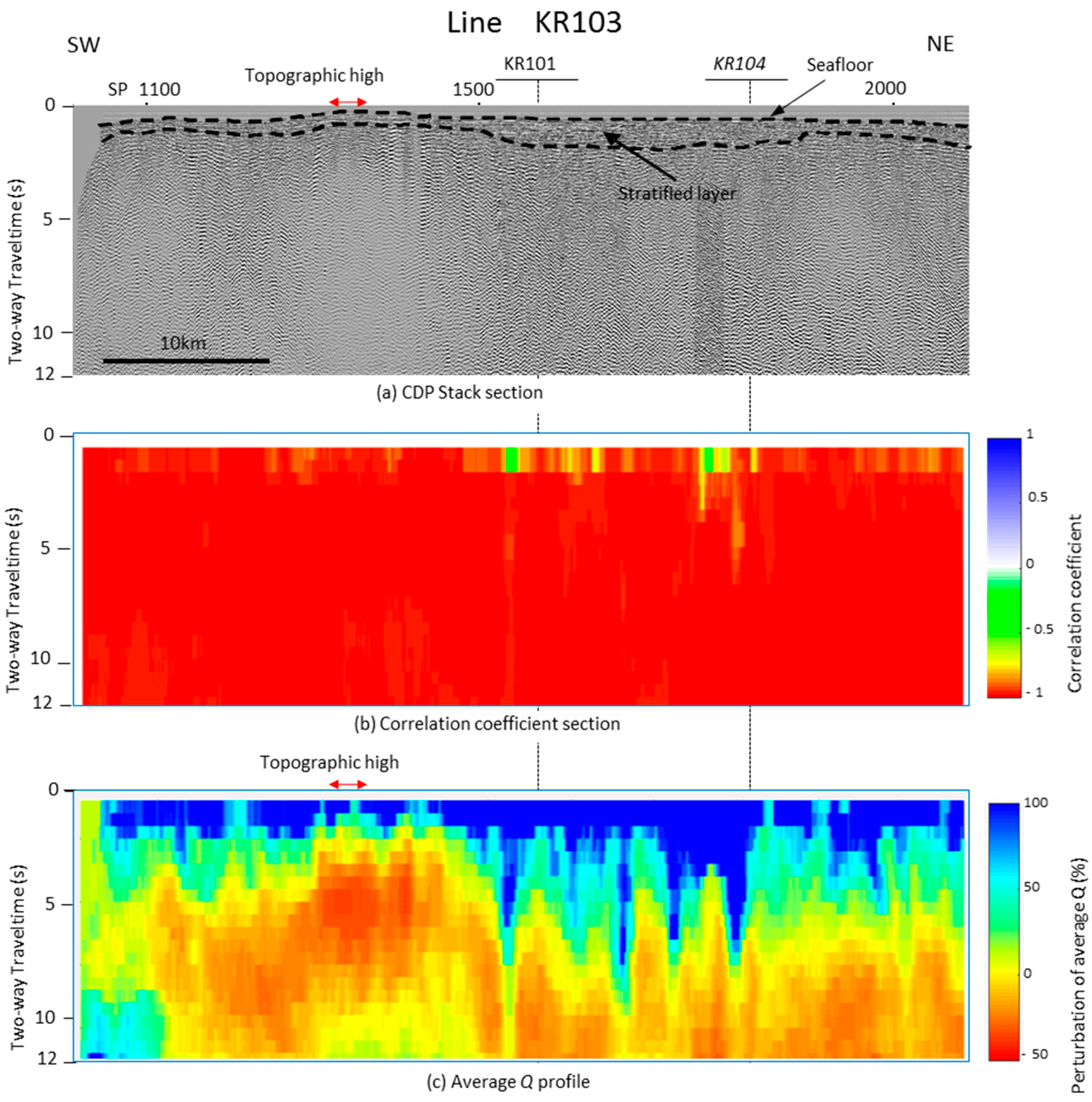
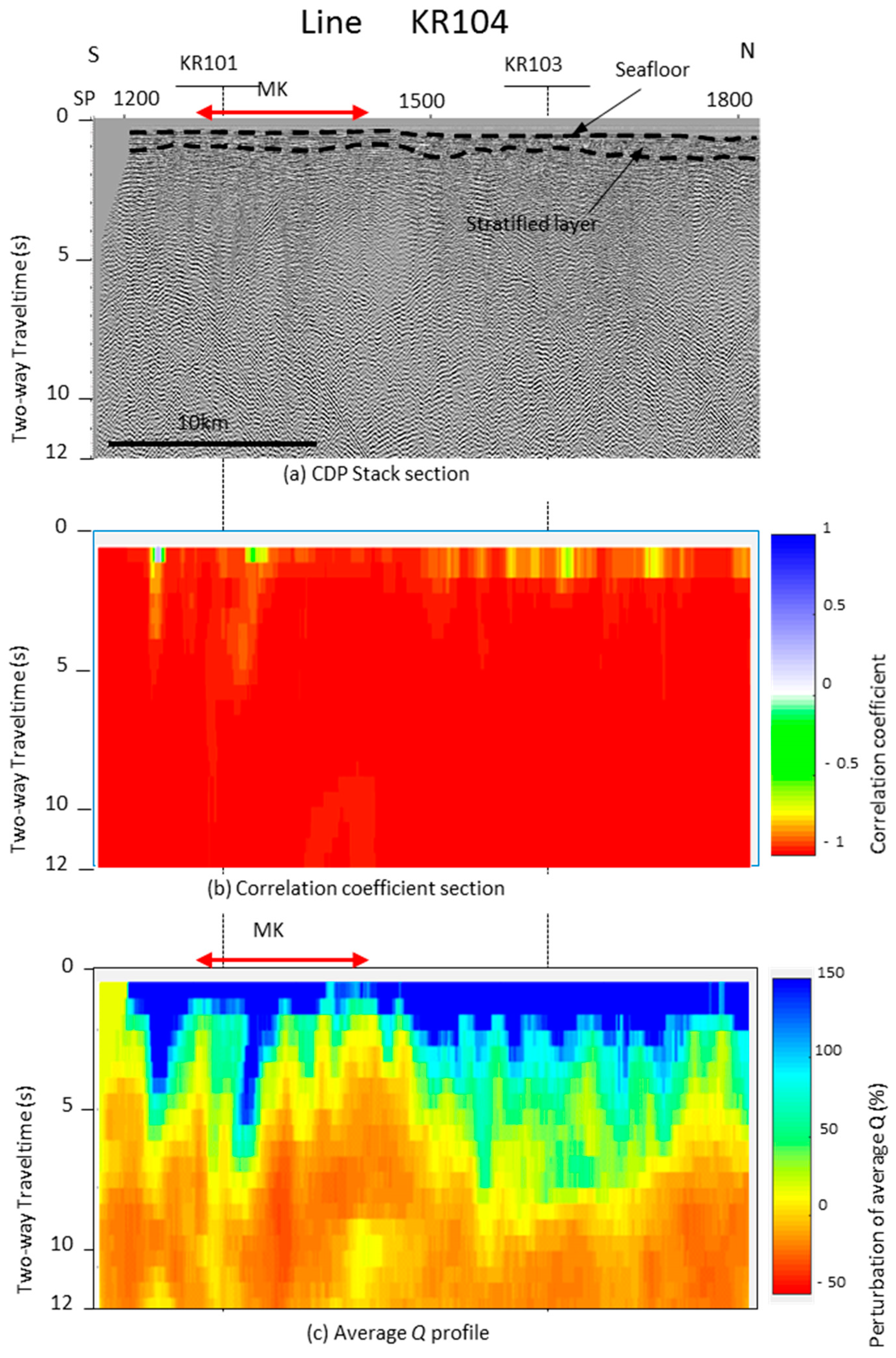
An up-warping high-attenuation anomaly was newly imaged beneath the topographic high on KR103 (Figure 8c). Based on the geological feature of the study area, which is located on the northern part of the Izu Islands and consists of a chain of volcanic islands [11], it can be considered that this topographic high was formed by the same volcanism as the volcanic islands. Therefore, this up-warping, high-attenuation anomaly on KR103 may reflect one of the volcanic activities that have repeatedly occurred in this region. Another up-warping high-attenuation anomaly was observed on KR104 in the present study (Figure 9c). The location of the anomaly is relatively near the Miyakejima volcano (Figure 1). Although it is difficult to specify spatial variation in geologic structure by sparse 2D seismic grid, this high-attenuation anomaly on KR104 may reflect the same volcanism mentioned above, because of the similarity in location.

Here, we further consider what geological feature(s) the high-attenuation anomalies reflect. According to previous studies, high-attenuation property reflects volcanism [2], fault activity [14], and gas reservoir [6]. Regarding the gas reservoir, there are no gas fields in the study area; therefore, it cannot be considered as a candidate for the high-attenuation anomalies observed in the present study. Fault activity associated with earthquake swarm becomes a possible candidate. However, no precise hypocenter distributions of earthquake swarms have been measured in the study area before the 2000 earthquake swarm occurred. Because only the hypocenter distribution of the 2000 swarm is available, the justification of the high-attenuation anomalies by fault activity is limited to only a few locations along the seismic lines.

On the other hand, volcanism is the most dominant geological feature in the study area [11], being applicable to every location in the study area. Concerning the vertical high-attenuation anomaly on KR102, its shape is very similar to that of the dike inclusion of magma associated with the 2000 Miyakejima eruption, which was deduced by the previous studies [5]. Regarding the up-warping, high-attenuation anomalies on KR103 and KR104, it is presently difficult to explain their causes by faults because their locations do not relate to the hypocenter distribution of the 2000 swarm. However, the anomaly on KR103 is located on the topographic high, suggesting volcanic activity and the anomaly on KR104 near the Miyakejima volcano. Thus, volcanism, which has been repeatedly occurred in this region, is likely the candidate cause of the high-attenuation anomalies newly observed in the present study.

As mentioned above, our observations suggest a relationship between the high-attenuation anomalies and volcanic activity along KR103 and KR104. This relationship suggests the presence of porous lithology that is often the result of volcanism.

5. Conclusions

Data preprocessing was revaluated to improve frequency preservation when handling input seismic data for SAP analysis. Deconvolution was excluded from the processing sequence, and NMO correction was applied with a very small stretching factor of 0.1. The resulting attenuation profiles successfully imaged the following high-attenuation anomalies that were not identified in the previous studies.

• A vertical high-attenuation anomaly on KR102 that probably reflected a cross section of the hypocenter distribution of the 2000 earthquake swarm.
• High-attenuation anomalies on KR103 and KR104 that likely reflected the volcanic activities that have repeatedly occurred in this region.

Although further investigation is still needed, this study demonstrated that our altered preprocessing improved the accuracy of geological structural imaging by SAP.

References

1. Tokuyama, H.; Suyehiro, K.; Watanabe, H.; Ohnishi, M.; Takahashi, A.; Ikawa, T.; Asada, M.; Fujioka, K.; Ashi, J.; Kuramoto, S.; et al. Multichannel seismic reflection profile from south of the Izu Oshima. J. Volcanol. Soc. Jpn. 1988, 33, 67–77, (In Japanese with English abstract). [Google Scholar]
2. Mikada, H.; Watanabe, H.; Sakashita, S. Evidence for subsurface magma bodies beneath Izu-Oshima, volcano inferred from a seismic scattering analysis and possible interpretation of the magma plumbing system of the 1986 eruptive activity. Phys. Earth Planet. Inter. 1997, 104, 257–269. [Google Scholar] [CrossRef]
3. Tsuru, T.; No, T.; Fujie, G. Geophysical imaging of subsurface structures in volcanic area by seismic attenuation profiling. Earth Planets Space 2017, 69. [Google Scholar] [CrossRef]
4. Sakai, S.; Yamada, T.; Ide, S.; Mochizuki, M.; Shiobara, H.; Urabe, T.; Hirata, N.; Shinohara, M.; Kanazawa, T.; Nishizawa, A.; et al. Magma migration from the point of view of seismic activity in the volcanism of Miyake-jima island in 2000. J. Geogr. 2001, 110, 145–155, (In Japanese with English abstract). [Google Scholar] [CrossRef]
5. Yamaoka, K.; Kudo, T.; Kawamura, M.; Kimata, F.; Fujii, N. Dike intrusion associated with the 2000 eruption of Miyakejima Volcano. Jpn. Bull. Volcanol. 2005, 67, 231–242. [Google Scholar] [CrossRef]
6. Dasgupta, R.; Clark, R.A. Estimation of Q from surface seismic reflection data. Geophysics 1998, 63, 2120–2128. [Google Scholar] [CrossRef]
7. Knopoff, L. Q. Rev. Geophys. 1964, 2, 625–660. [Google Scholar] [CrossRef]
8. Mavko, G.M.; Nur, A. Wave attenuation in partially saturated rocks. Geophysics 1979, 44, 161–178. [Google Scholar] [CrossRef]
9. Hauge, P.S. Measurements of attenuation from vertical seismic profiles. Geophysics 1981, 46, 1548–1558. [Google Scholar] [CrossRef]
10. Tonn, R. The determination of seismic quality factor Q from VSP data: A comparison of different computational methods. Geophys. Prospect. 1991, 39, 1–27. [Google Scholar] [CrossRef]
11. Hamada, N. A history of seismic activity around Miyakejima, Kozushima and Niijima, the northern Izu islands. J. Geogr. 2001, 110, 132–144, (In Japanese with English abstract). [Google Scholar] [CrossRef]
12. Uhira, K.; Baba, T.; Mori, M.; Katayama, H.; Hamada, N. Earthquake swarms preceding the 2000 eruption of Miyakejima volcano. Jpn. Bull. Volcanol. 2005, 67, 219–230. [Google Scholar] [CrossRef]
13. Nishizawa, A.; Ono, T.; Otani, Y. Seismicity and crustal structure related to the Miyake-jima volcanic activity in 2000. Geophys. Res. Lett. 2002, 29. [Google Scholar] [CrossRef]
14. Blakeslee, S.; Malin, P.; Alvarez, M. Fault-zone attenuation of high-frequency seismic waves. Geophys. Res. Lett. 1989, 16, 1321–1324. [Google Scholar] [CrossRef]
Figure 1. Study area and seismic reflection survey lines (modified the previous study [3]). Four lines of seismic reflection data were collected during the KR00-08 Cruise of R/V Kairei by Japan Agency of Marine-Earth Science and Technology (JAM STEC) in 2000. The three thick blue lines represent seismic lines used in this study. The 4-digit numbers show Shot Point (SP) number.
Geosciences 08 00038 g001
Figure 2. Hypocenter distribution of the earthquake swarm in 2000 [4] and seismic lines in Figure 1. The hypocenters determined by both land stations and Ocean Bottom Seismometers (OBSs) in 2000 are shown in the left side map. The four seismic lines were overlaid on the map. The right figures represent the hypocenters projected to the cross sections of A,B and C,D, indicating a dike intrusion of magma associated with the 2000 eruption of Miyakejima Volcano [5].
Geosciences 08 00038 g002
Figure 3. Flow chart of the preprocessing of seismic reflection data for the present SAP study (modified after the previous study [3]). To avoid the frequency distortion of reflections, deconvolution was excluded in the preprocessing sequence for SAP analysis. NMO correction was applied with a very small stretching factor of 0.1, which did not allow NMO stretch to exceed 10%.
Geosciences 08 00038 g003
Figure 4. An example of frequency distortion by deconvolution. The black solid shows spectrum before deconvolution, whereas the red broken line is that after deconvolution. The frequency components of 30–50 Hz are raised by the deconvolution. Those spectrums were calculated in a time window 2–3 s at SP1500 of KR102.
Geosciences 08 00038 g004
Figure 5. An example of frequency distortion by NMO stretch factor on spectrum (a) and CDP gather (b). The black solid line, red solid line, and blue dot line in the top figure (a) show spectrums from stretch factors of 0.5, 0.1, and 0.05, respectively.
Geosciences 08 00038 g005
Figure 6. An example of gradient p computation and correlation coefficient of linear approximation. The black solid curve shows the logarithm of the spectral ratio function of frequency (10–30 Hz) in a time window 7.680–8.192 s at the location of CDP1700. The orange broken line is a straight line with gradient p, which was computed by linear approximation with the least squares method. The correlation coefficient of the approximation was −0.9963.
Geosciences 08 00038 g006
Figure 7. CDP stack section (a), correlation coefficient section (b), and average Q profile (c) of line KR102. The stratified layer with continuous reflections was imaged in the shallowest part on the CDP stack section; however, no reflections can be observed below the layer. The correlation coefficient section shows that almost all of the correlation coefficients in the linear approximation of gradient p represent highly negative correlations (less than −0.8). A vertical high attenuation anomaly was clearly imaged on the average Q profile near the intersection with KR101.
Geosciences 08 00038 g007
Figure 8. CDP stack section (a), correlation coefficient section (b), and average Q profile (c) of line KR103. The stratified layer with continuous reflections was imaged in the shallowest part on the CDP stack section; however, no reflections can be observed below the layer. The correlation coefficient section shows that almost all of the correlation coefficients in the linear approximation of gradient p represent highly negative correlations (less than −0.8). An up-warping high attenuation anomaly can be observed on the average Q profile on the topographic high (see Figure 1).
Geosciences 08 00038 g008
Figure 9. CDP stack section (a), correlation coefficient section (b), and average Q profile (c) of line KR104. The stratified layer with continuous reflections was imaged in the shallowest part on the CDP stack section; however, no reflections can be observed below the layer. The correlation coefficient section shows that almost all of the correlation coefficients in the linear approximation of gradient p represent highly negative correlations (less than −0.8). An up-warping high attenuation anomaly can be observed on the average Q profile near the Miyakejima volcano (see Figure 1).
Geosciences 08 00038 g009