How to Define Priorities in Coastal Vulnerability Assessment


Abstract
:1. Introduction
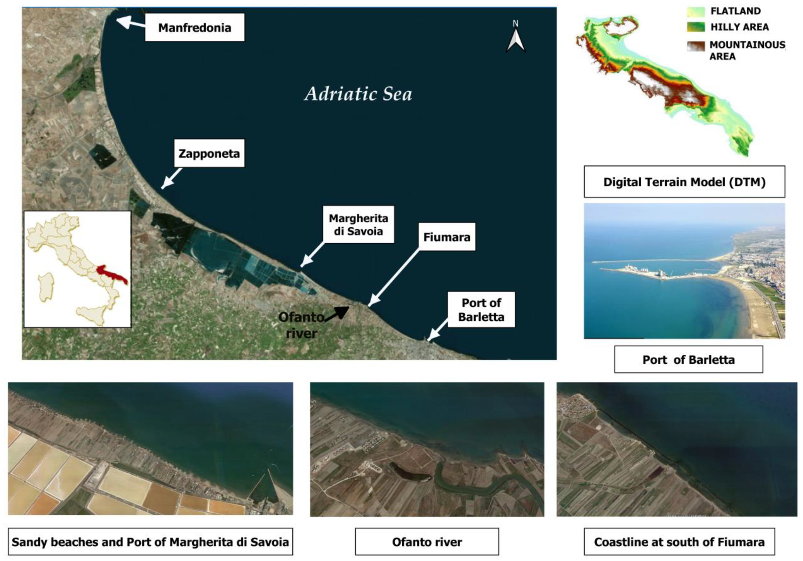
2. Study Area
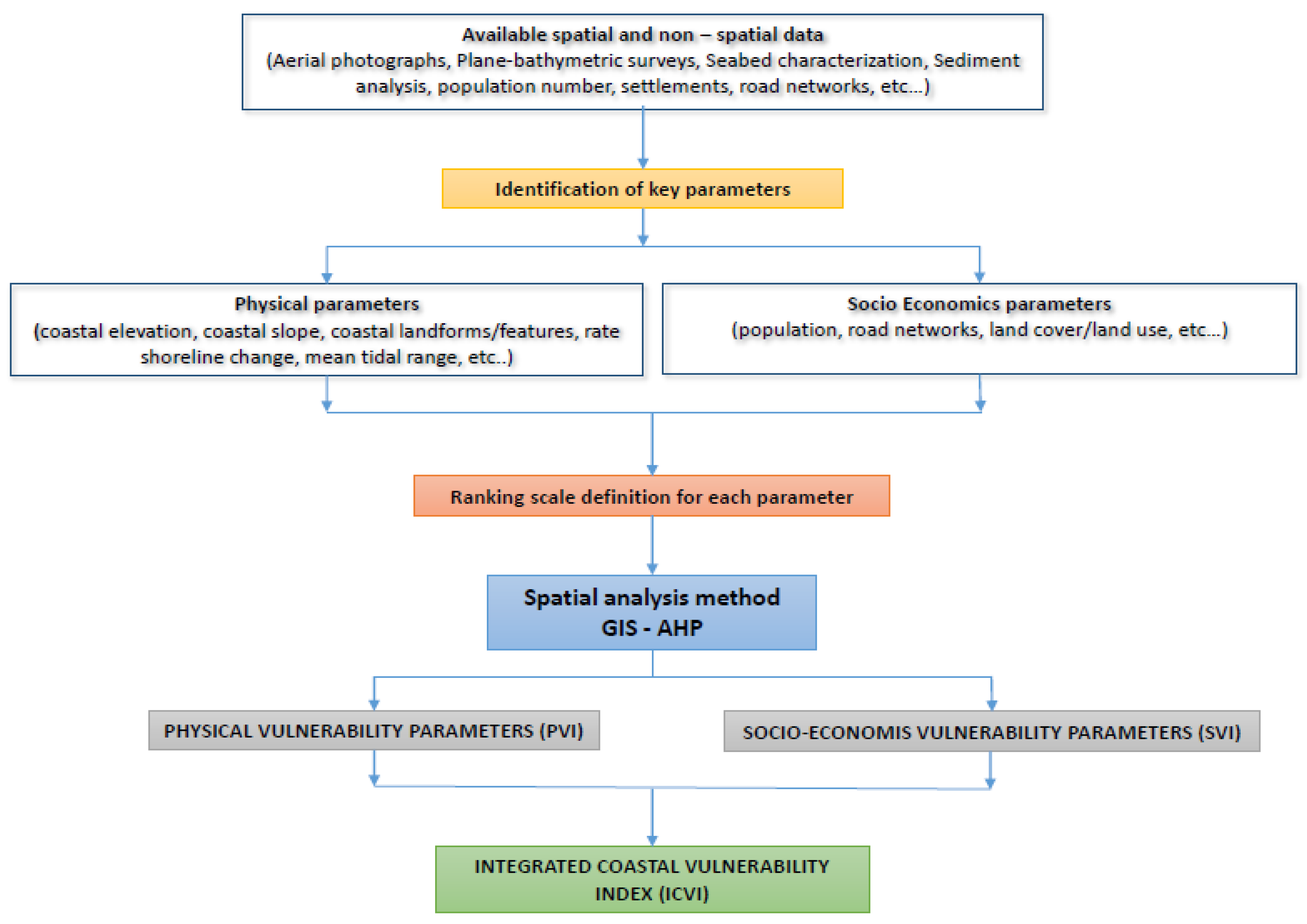
3. Materials and Methods
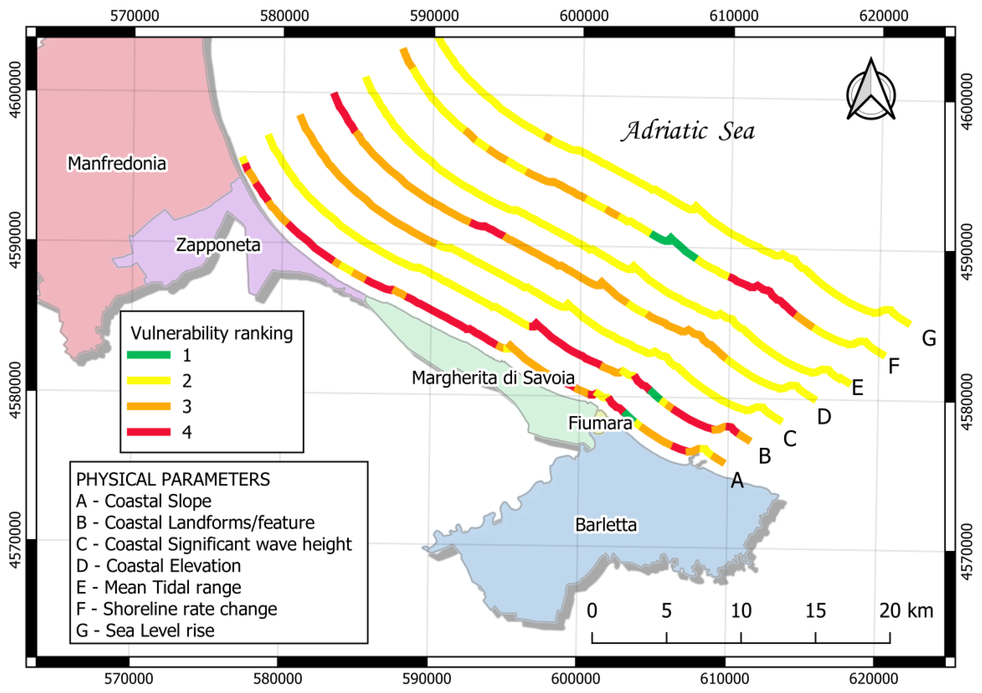
3.1. Physical Parameters
3.1.1. Coastal Slope
3.1.2. Coastal Landforms/Features
3.1.3. Significant Wave height
3.1.4. Shoreline Change Rate
3.1.5. Sea Level Rise
3.1.6. Tidal Level
3.1.7. Coastal Elevation
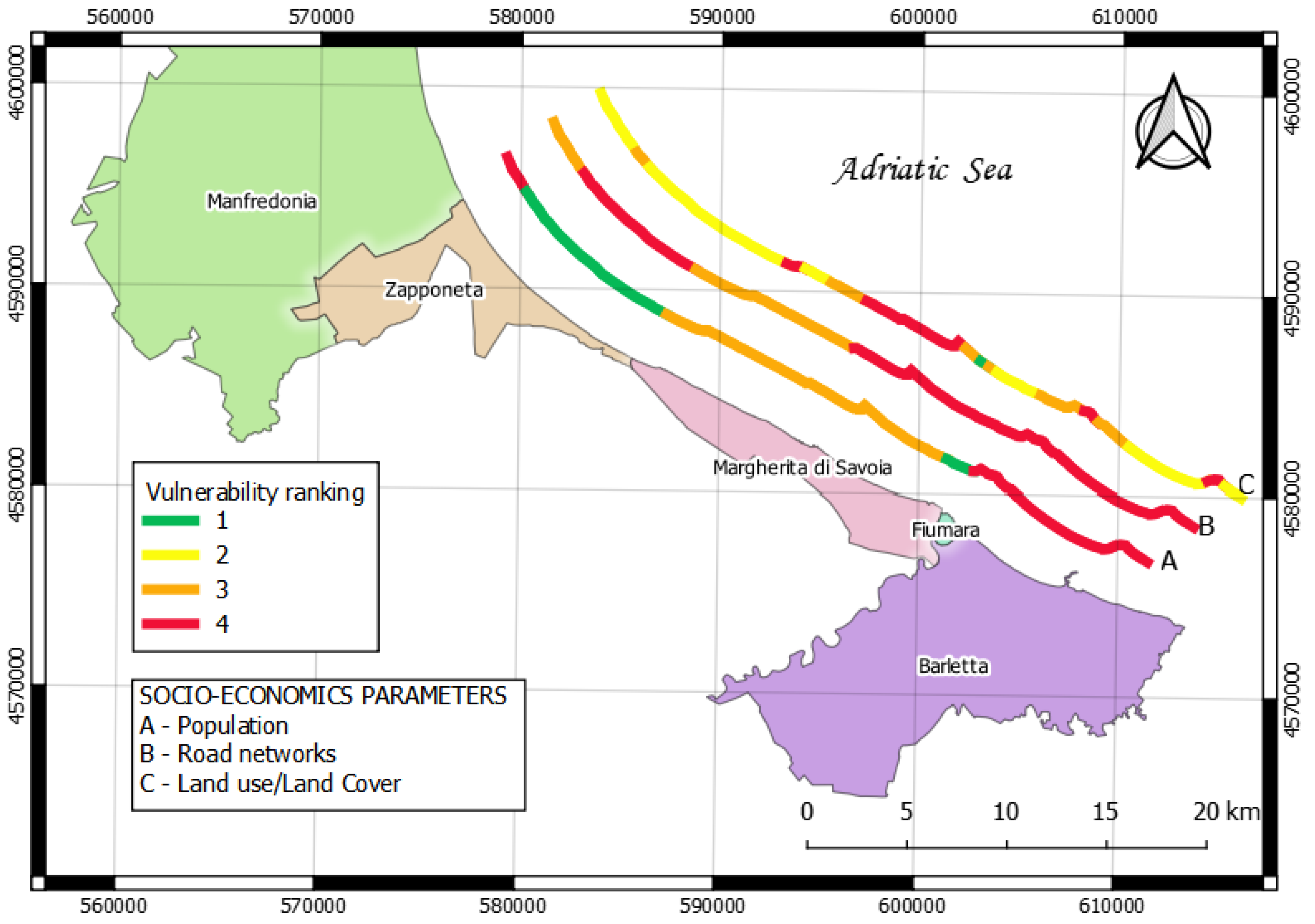
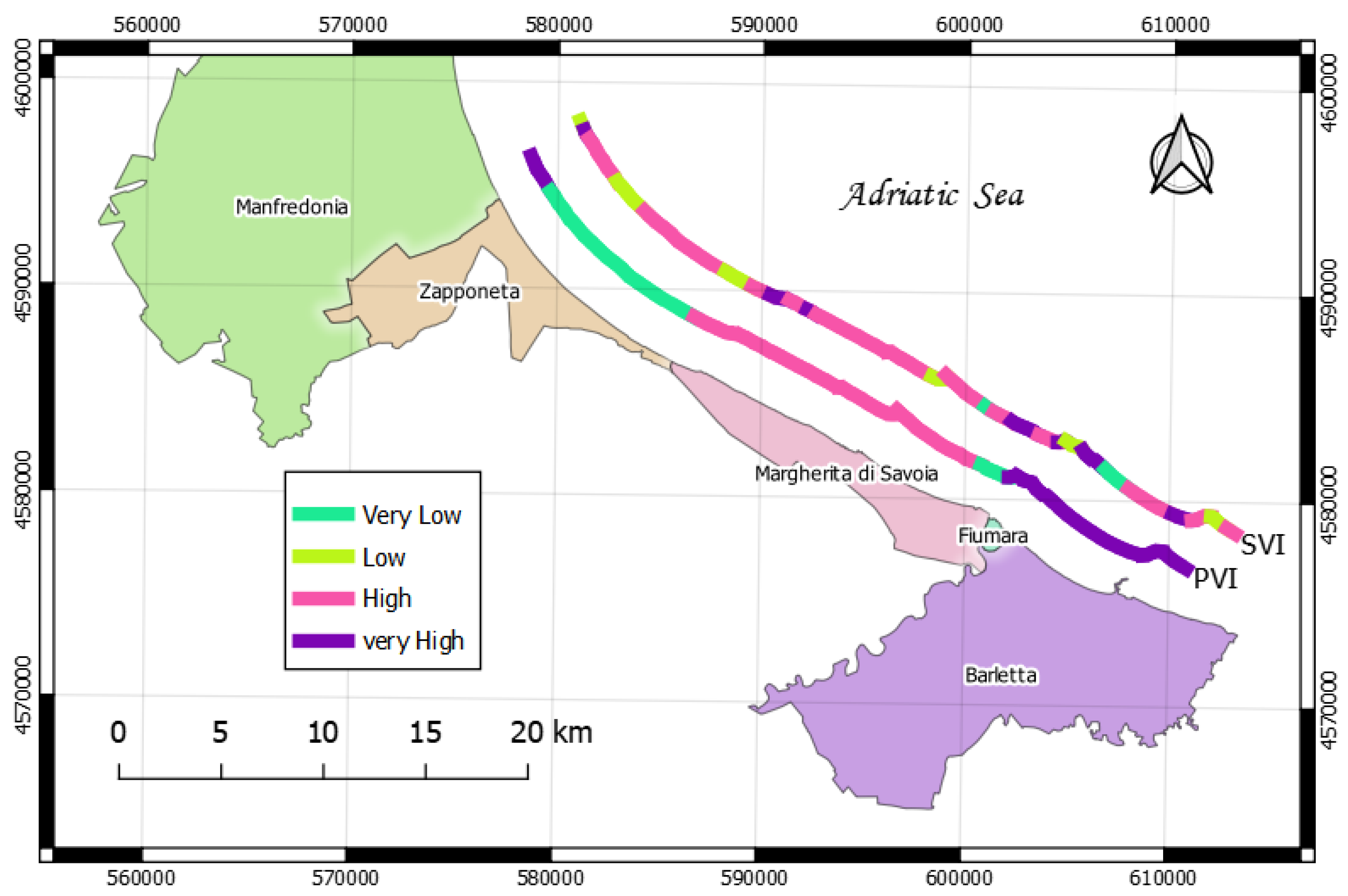
3.2. Socio-Economic Parameters
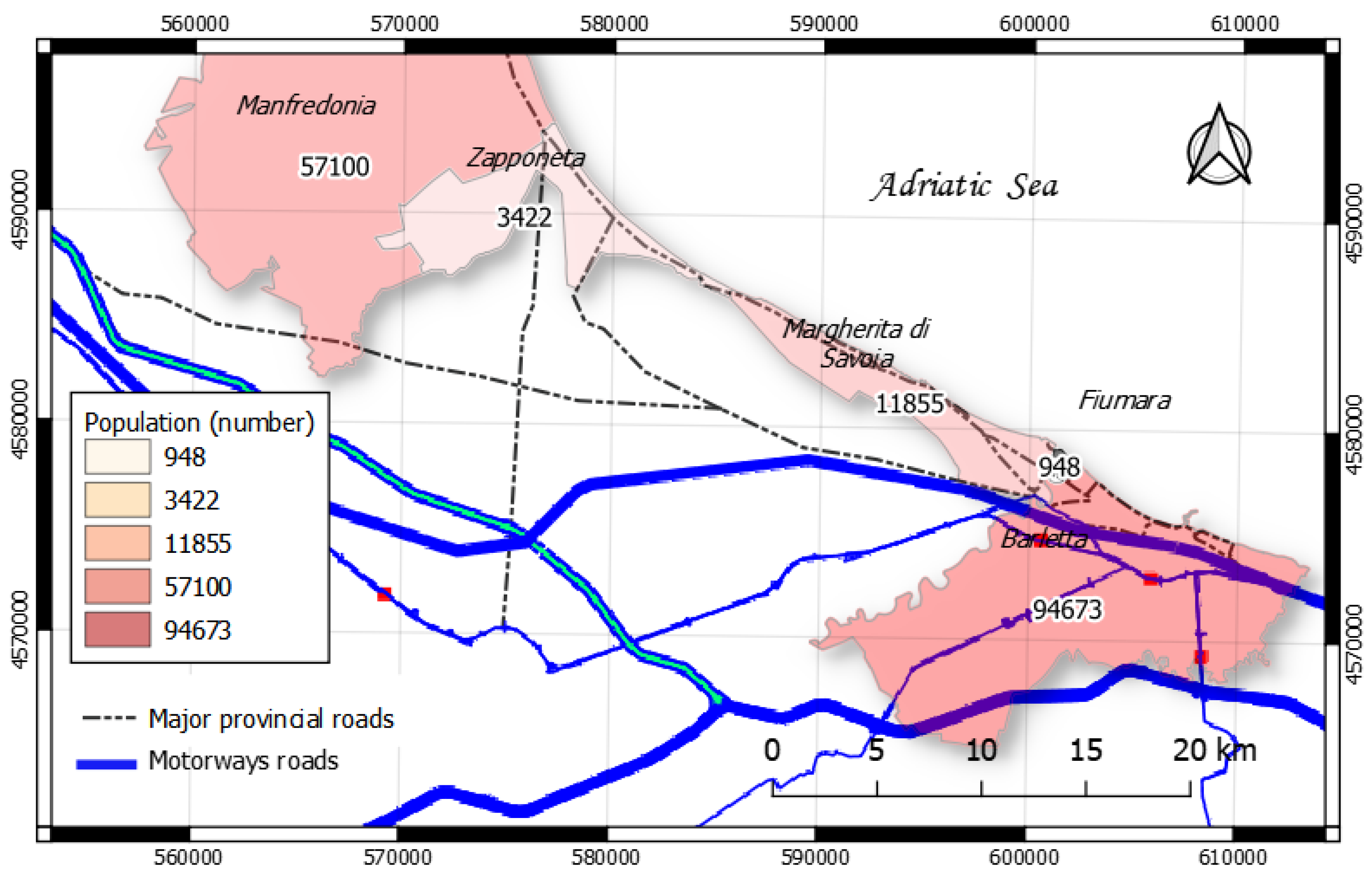
3.2.1. Population
3.2.2. Coastal Road Networks
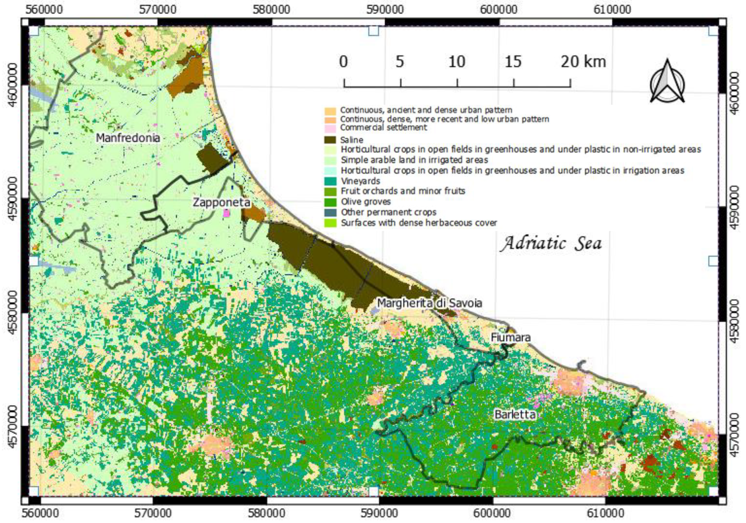
3.2.3. Land Use/Land Cover
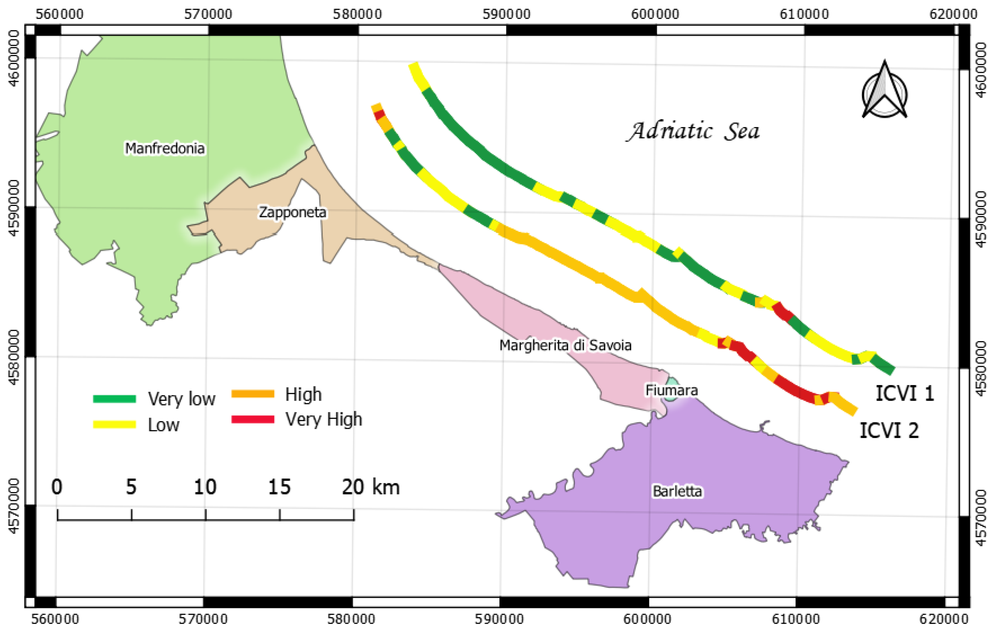
3.3. Analytical Hierarchical Process
4. Results and Discussion
5. Conclusions
Author Contributions
Funding
Conflicts of Interest
References
- Pramanik, M.K.; Biswas, S.S.; Mondal, B.; Pal, R. Coastal vulnerability assessment of the predicted sea level rise in the coastal zone of Krishna–Godavari delta region, Andhra Pradesh, east coast of India. Environ. Dev. Sustain. 2016, 18, 1635–1655. [Google Scholar] [CrossRef]
- Feola, A.; Lisi, I.; Salmeri, A.; Venti, F.; Pedroncini, A.; Gabellini, M.; Romano, E. Platform of integrated tools to support environmental studies and management of dredging activities. J. Environ. Manag. 2016, 166, 357–373. [Google Scholar] [CrossRef] [PubMed]
- IPCC. Summary for policymakers. In Climate Change 2014: Impacts, Adaptation, and Vulnerability. Part A: Global and Sectoral Aspects. Contribution of Working Group II to the Fifth Assessment Report of the Intergovernmental Panel on Climate Change; Field, C.B., Barros, V.R., Dokken, D.J., Mach, K.J., Mastrandrea, M.D., Bilir, T.E., Chatterjee, M., Ebi, K.L., Estrada, Y.O., Genova, R.C., et al., Eds.; Cambridge University Press: Cambridge, UK; New York, NY, USA, 2014; pp. 1–32. [Google Scholar]
- Torresan, S.; Critto, A.; Rizzi, J.; Marcomini, A. Assessment of coastal vulnerability to climate change hazards at the regional scale: The case study of the north Adriatic Sea. Nat. Hazards Earth Syst. Sci. 2012, 12, 2347–2368. [Google Scholar] [CrossRef] [Green Version]
- Galassi, G.; Spada, G. Sea-level rise in the Mediterranean Sea by 2050: Roles of terrestrial ice melt, steric effects and glacial isostatic adjustment. Glob. Planet. Chang. 2014, 123, 55–66. [Google Scholar] [CrossRef]
- Pickering, M.D.; Horsburgh, K.J.; Blundell, J.R.; Hirschi, J.M.; Nicholls, R.J.; Verlaan, M.; Wells, N.C. The impact of future sea-level rise on the global tides. Cont. Shelf Res. 2017, 142, 50–68. [Google Scholar] [CrossRef] [Green Version]
- McLean, R.; Tsyban, A.; Burkett, V.; Codignotto, J.O.; Forbes, D.L.; Mimura, N.; Beamish, R.J.; Ittekkot, V. Coastal zone and marine ecosystems. In Climate Change 2001: Impacts, Adaptation and Vulnerability; McCarthy, J.J., Canziani, O.F., Leary, N.A., Dokken, D.J., White, K.S., Eds.; Cambridge University Press: Cambridge, UK, 2001; pp. 343–380. [Google Scholar]
- Martínez-Graña, A.; Gómez, D.; Santos-Francés, F.; Bardají, T.; Goy, J.L.; Zazo, C. Analysis of flood risk due to sea level rise in the Menor Sea (Murcia, Spain). Sustainability 2018, 10, 780. [Google Scholar] [CrossRef]
- Torresan, S.; Critto, A.; Dalla Valle, M.; Harvey, N.; Marcomini, A. Assessing coastal vulnerability to climate change: Comparing segmentation at global and regional scales. Sustain. Sci. 2008, 3, 45–65. [Google Scholar] [CrossRef]
- Armenio, E.; De Serio, F.; Mossa, M. Analysis of data characterizing tide and current fluxes in coastal basins. Hydrol. Earth Syst. Sci. 2017, 21, 3441–3454. [Google Scholar] [CrossRef] [Green Version]
- Maanan, M.; Rueff, H.; Adouk, N.; Zourarah, B.; Rhinane, H. Assess the human and environmental vulnerability for coastal hazard by using a multi-criteria decision analysis. Hum. Ecol. Risk Assess. Int. J. 2018, 24, 1642–1658. [Google Scholar] [CrossRef]
- ETC CCA. Methods for Assessing Coastal Vulnerability to Climate Change. Technical Paper 1/2011. Available online: http://cca.eionet.europa.eu/docs/TP_1-2011 (accessed on 20 September 2018).
- Bosom, E.; Jimenez, J.A. Probabilistic coastal vulnerability assessment to storms at regional scale e application to Catalan beaches (NW Mediterranean). Nat. Hazards Earth Syst. Sci. 2011, 11, 475–484. [Google Scholar] [CrossRef] [Green Version]
- Shanganlall, A.; Ferentinou, M.; Karymbalis, E.; Smith, A. A Coastal Susceptibility Index Assessment of KwaZulu-Natal, East Coast of South Africa. In IAEG/AEG Annual Meeting Proceedings, San Francisco, California; Springer: Cham, Switzerland, 2018; Volume 5, pp. 93–100. [Google Scholar]
- Gornitz, V.M. Global coastal hazards from future sea level rise. Glob. Planet. Chang. 1991, 3, 379–398. [Google Scholar] [CrossRef]
- Gornitz, V.M.; White, T.W.; Cushman, R.M. Vulnerability of the U.S. to future sea-level rise. In Proceedings of the Seventh Symposium on Coastal and Ocean Management, Long Beach, CA, USA, 8–12 July 1991; pp. 2354–2368. [Google Scholar]
- Thieler, E.R.; Hammar-Klose, E.S. National Assessment of Coastal Vulnerability to Future Sea-Level Rise: Preliminary Results for the U.S. Gulf of Mexico Coast; U.S. Geological Survey, Open-File Report; 2000. Available online: http://pubs.usgs.gov/of/of00-179 (accessed on 20 September 2018).
- Thieler, E.R.; Hammar-Klose, E.S. National Assessment of Coastal Vulnerability to Sea-Level Rise: Preliminary Results for the U.S. Atlantic Coast; U.S. Geological Survey, Open-File Report; 1999. Available online: https://pubs.usgs.gov/of/1999/of99-593 (accessed on 20 September 2018).
- Vittal Hegde, A.; Radhakrishnan Reju, V. Development of Coastal Vulnerability Index for Mangalore Coast, India. J. Coast. Res. 2007, 23, 1106–1111. [Google Scholar] [CrossRef]
- Nageswara Rao, K.; Subraelu, P.; Venkateswara Rao, T.; Hema Malini, B.; Ratheesh, R.; Bhattacharya, S.; Rajawat Ajai, A.J. Sea-level rise and coastal vulnerability: An assessment of Andhra Pradesh coast, India through remote sensing and GIS. J. Coast. Conserv. 2008, 12, 195–207. [Google Scholar] [CrossRef]
- Casini, M.; Mocenni, C.; Paoletti, S.; Vicino, A. A decision support system for the management of coastal lagoons. In Proceedings of the 16th IFAC World Congress, Prague, Czech Republic, 4—8 July 2005. [Google Scholar]
- Hinkel, J. DIVA: An iterative method for building modular integrated models. Adv. Geosci. 2005, 4, 45–50. [Google Scholar] [CrossRef]
- Alexandrakis, G.; Poulos, S.Е. An holistic approach to beach erosion vulnerability assessment. Sci. Rep. 2014, 4, 6078. [Google Scholar] [CrossRef] [PubMed]
- McLaughlin, S.; McKenna, J.; Cooper, J.A.G. Socio-economic data in coastal vulnerability indices: Constraints and opportunities. J. Coast. Res. 2002, 36, 487–497. [Google Scholar] [CrossRef]
- Tragaki, A.; Gallousi, C.; Karymbalis, E. Coastal Hazard Vulnerability Assessment Based on Geomorphic, Oceanographic and Demographic Parameters: The Case of the Peloponnese (Southern Greece). Land 2018, 7, 56. [Google Scholar] [CrossRef]
- Zahedi, F. The analytic hierarchy process. A survey of the method and its applications. Interfaces 1986, 16, 96–108. [Google Scholar] [CrossRef]
- Vaidya, O.S.; Kumar, S. Analytic hierarchy process: An overview of applications. Eur. J. Oper. Res. 2006, 169, 1–29. [Google Scholar] [CrossRef]
- Fierro, G.; Ivaldi, R. The Atlas of the Italian Beaches: A review of coastal processes. MEDCOAST 2001, 1, 1557–1566. [Google Scholar]
- Anfuso, G.; Martinez, J.A.; Nachite, D. Coastal vulnerability in the Mediterranean sector between Fnideq and M’diq (North of Morocco). C. R. Acad. Bulg. Sci. 2010, 63, 561–570. [Google Scholar]
- Bhatt, R.; Macwan, J.E.M.; Bhatt, D.; Patel, V. Analytic hierarchy process approach for criteria ranking of sustainable building assessment: A case study. World Appl. Sci. J. 2010, 8, 881–888. [Google Scholar]
- Di Paola, G.; Aucelli, P.P.C.; Benassai, G.; Rodríguez, G. Coastal vulnerability to wave storms of Sele littoral plain (southern Italy). Nat. Hazards 2014, 71, 1795–1819. [Google Scholar] [CrossRef]
- Murali, R.M.; Ankita, M.; Amrita, S.; Vethamony, P. Coastal vulnerability assessment of Puducherry coast, India, using the analytical hierarchical process. Nat. Hazards Earth Syst. Sci. 2013, 13, 3291–3311. [Google Scholar] [CrossRef] [Green Version]
- Le Cozannet, G.L.; Garcin, M.; Bulteau, T.; Mirgon, C.; Yates, M.L.; Méndez, M.; Baills, A.; Idier, D.; Oliveros, C. An AHP-derived method for mapping the physical vulnerability of coastal areas at regional scales. Nat. Hazards Earth Syst. Sci. 2013, 13, 1209–1227. [Google Scholar] [CrossRef] [Green Version]
- Gutierrez, B.T.; Williams, S.J.; Thieler, E.R. Expert Panel Assessment of Potential Shoreline Changes Due to Sea-Level Rise Along the U.S. Mid-Atlantic Region; USGS Open File Report; 2007. Available online: https://woodshole.er.usgs.gov/pubs/of2007-1278 (accessed on 20 September 2018).
- Saaty, T.L. A scaling method for priorities in hierarchical structures. J. Math. Psychol. 1977, 15, 234–281. [Google Scholar] [CrossRef]
- Saaty, T.L.; Vargas, L.G. Prediction, Projection, and Forecasting: Applications of the Analytic Hierarchy Process in Economics, Finance, Politics, Games, and Sport; Springer Netherlands: Heidelberg, Germany, 1991. [Google Scholar]
- Ju, C.Y.; Jia, Y.G.; Shan, H.X.; Tang, C.W.; Ma, W.J. GIS-based coastal area suitability assessment of geo-environmental factors in Laoshan district, Qingdao. Nat. Hazards Earth Syst. Sci. 2012, 12, 143–150. [Google Scholar] [CrossRef] [Green Version]
- Phukon, P.; Chetia, D.; Das, P. Landslide susceptibility assessment in the Guwahati city, Assam using analytic hierarchy process (AHP) and geographic information system (GIS). Int. J. Comput. Appl. Eng. Sci. 2012, 2, 1–6. [Google Scholar]
- Rahman, M.R.; Shi, Z.H.; Chongfa, C. Soil erosion hazard evaluation—An integrated use of remote sensing, GIS and statistical approaches with biophysical parameters towards management strategies. Ecol. Model. 2009, 220, 1724–1734. [Google Scholar] [CrossRef]
- Kaly, U.L.; Pratt, C.R.; Mitchell, J. The Environmental Vulnerability Index (EVI). SOPAC Technical Report 384. 2004. Available online: http://www.sopac.org/sopac/evi/Files/EVI2004 (accessed on 20 September 2018).
- Adger, N.; Vincent, K. Uncertainty in adaptive capacity. C. R. Geosci. 2005, 337, 399–410. [Google Scholar] [CrossRef]
- Payo, A.; Hall, J.W.; French, J.; Sutherland, J.; van Maanen, B.; Nicholls, R.J.; Reeve, D.E. Causal loop analysis of coastal geomorphological systems. Geomorphology 2016, 256, 36–48. [Google Scholar] [CrossRef]
- Karymbalis, E.; Chalkias, C.; Chalkias, G.; Grigoropoulou, E.; Manthos, G.; Ferentinou, M. Assessment of the Sensitivity of the Southern Coast of the Gulf of Corinth (Peloponnese, Greece) to Sea-level Rise. Cent. Eur. J. Geosci. 2012, 4, 561–577. [Google Scholar] [CrossRef]
- Lambeck, K.; Antonioli, F.; Anzidei, M.; Ferranti, L.; Leoni, G.; Scicchitano, G.; Silenzi, S. Sea level change along the Italian coast during the Holocene and projections for the future. Quat. Int. 2011, 232, 250–257. [Google Scholar] [CrossRef]
- Pendleton, E.A.; Thieler, E.R.; Williams, S.J. Coastal Vulnerability Assessment of Cape Hettaras National Seashore (CAHA) to Sea Level Rise; USGS Open File Report; 2005. Available online: https://pubs.usgs.gov/of/2004/1064/ (accessed on 20 September 2018).
- Valdmann, A.; Käärd, A.; Kelpšaitė, L.; Kurennoy, D.; Soomere, T. Marine coastal hazards for the eastern coasts of the Baltic Sea. Baltica 2008, 21, 3–12. [Google Scholar]
- Armenio, E.; De Serio, F.; Mossa, M.; Nobile, B.; Petrillo, A.F. Investigation on coastline evolution using long-term observations and numerical modelling. In Proceedings of the 27th International Ocean and Polar Engineering Conference, San Francisco, CA, USA, 25–30 June 2017. [Google Scholar]
- Žilinskas, G.; Jarmalavičius, D. Estimation of vulnerability of Lithuanian Baltic sea coasts on the background of Baltic Sea water level rise. Geografijos Metraštis 1996, 29, 174–183. [Google Scholar]
- Pranzini, E.; Williams, A. Coastal Erosion and Protection in Europe; Routledge, Taylor and Francis: Abingdon, UK; New York, NY, USA, 2013. [Google Scholar]
- Raicich, F. Recent evolution of sea-level extremes at Trieste (Northern Adriatic). Cont. Shelf Res. 2003, 23, 225–235. [Google Scholar] [CrossRef]
- Bruno, M.F.; Molfetta, M.G.; Petrillo, A.F. The influence of interannual variability of mean sea level in the Adriatic Sea on extreme values. J. Coast. Res. 2014, 70, 241–246. [Google Scholar] [CrossRef]
- Solomon, S. Climate Change 2007-the Physical Science Basis: Working Group I Contribution to the Fourth Assessment Report of the IPCC; Cambridge University Press: Cambridge, UK; New York, NY, USA, 2007; Volume 4. [Google Scholar]
- Petrillo, A.F. Coastal areas: Current and future critical issues. In Geologists and Territory; Magazine of the Order of Geologists of Puglia: Bari, Italy, 2007; pp. 117–130. [Google Scholar]
- Szlafsztein, C.; Sterr, H. A GIS-based vulnerability assessment of coastal natural hazards, state of Pará, Brazil. J. Coast. Conserv. 2007, 11, 53–66. [Google Scholar] [CrossRef]
- Devoy, R.J. Questions of coastal protection and the human response to sea-level rise in Ireland and Britain. Ir. Geogr. 1992, 25, 1–22. [Google Scholar] [CrossRef]
- Dilley, R.S.; Rasid, H. Human response to coastal erosion: Thunder bay, Lake Superior. J. Coast. Res. 1990, 6, 779–788. [Google Scholar]
- Mahapatra, M.; Ratheesh, R.; Rajawat, A.S. Shoreline change analysis along the coast of South Gujarat, India, using digital shoreline analysis system. J. Indian Soc. Remote Sens. 2014, 42, 869–876. [Google Scholar] [CrossRef]
- Mu, E.; Pereyra-Rojas, M. Practical Decision Making; Springer Briefs in Operations Research; Springer Nature: Basel, Switzerland, 2017. [Google Scholar]
- Cogswell, A.; Blair, J.W.; Greenan, P.G. Evaluation of two common vulnerability index calculation methods. Ocean Coast. Manag. 2018, 160, 46–51. [Google Scholar] [CrossRef]


| Variable | Data Source | Period of Reference | |
|---|---|---|---|
| Physical | Coastal slope | Atlas of Italian beaches Data from Territorial Information Service–Apulian Region (www.sit.puglia.it) | 2001 |
| Coastline landforms/features | Cartography and orthophoto from National Geoportal (http://www.pcn.minambiente.it) | 2005; 2008; 2011; 2013 | |
| Significant Wave height | European Centre for Medium-Range Weather Forecasts (ECMWF) model | 2008–2013 | |
| Shoreline change rate | Aerial photos (spatial), GPS measurements | 1992; 1997; 2005; 2008; 2011; 2013 | |
| Sea level rise | Literature data about the projections of global mean sea level rise over the 21st century (IPCC 2014; Galassi and Spada [5]; Lambeck et al. [44]) | 1990–2100 | |
| Tidal data | Tide gauge data from National tide gauge network (https://www.mareografico.it/) | 1999–2014 | |
| Coastal elevation | Data from Territorial Information Service–Apulian Region (www.sit.puglia.it) | 2015 | |
| Socio-economic | Population | Census sectors maps and Statistic data from National Institute of Statistics (https://www.istat.it/) | 2017 |
| Road networks | ANAS (http://stradeanas.it/it) | 2017 | |
| Land use/Land cover | Cartography from Ortho-images from National Geoportal (http://www.pcn.minambiente.it) Data from Territorial Information Service–Apulian Region (www.sit.puglia.it) | 2017 2011 |
| Parameter | Description | Coastal Vulnerability Ranking | |||
|---|---|---|---|---|---|
| Very Low (1) | Low (2) | High (3) | Very High (4) | ||
| Coastal slope (%) | Percentage of coastal slope | >2 | 1.3 ÷ 2 | 0.5 ÷ 1.3 | 0.1 ÷ 0.5 |
| Coastal landforms/features | Coastal resistance capacity against erodibility and sea level rise | Rocky coast | Protection works | Dunes, estuaries and lagoons | Mudflats, mangroves, beaches, barrier-spits |
| Significant wave height (m) | Significant wave height can cause severe coastal erosion | <0.55 | 0.55 ÷ 0.85 | 0.85 ÷ 1.2 | >1.2 |
| Shoreline change rate (m/year) | Mobility shoreline (positive accretion, negative erosion) | >+2 | +2 to 0 | 0 to −2 | <−2 |
| Sea level rise (mm/year) | Mean sea-level rise per year | <1.8 | 1.8 ÷ 2.6 | 2.6 ÷ 3.4 | >3.4 |
| Tidal range (m) | Difference between yearly mean high tide and low tide | <0.2 | 0.2 ÷ 0.45 | 0.45 ÷ 0.7 | >0.7 |
| Coastal elevation (m) | Surface elevation to mean sea level | >6 | 3 ÷ 6 | 0 ÷ 3 | <0 |
| Parameter | Description | Coastal Vulnerability Ranking | |||
|---|---|---|---|---|---|
| Very Low (1) | Low (2) | High (3) | Very High (4) | ||
| Population | Number of residents in the coastal municipality. | 0–5000 | 5000–10,000 | 10000–50,000 | >50,000 |
| Road networks (distance in km) | Presence of roads in coastal areas in terms of distance from the shoreline. | >1.5 | 1.5–1.0 | 1.0–0.5 | <0.5 |
| Land use/Land cover | Land use refers to purposes served by land (i.e., recreation, tourism, agriculture, residence). Land cover refers to surface cover on the ground (i.e., vegetation, urban infrastructure, water, bare soil or other). | Barren land, water bodies, marsh/bog and moor, sparsely vegetated areas, bare rock | Vegetated land or open spaces, Coastal area (tidal flats, mangroves, salt pans, beaches), natural grassland | Agriculture/fallow land | Urban, ecological sensitive regions. Urban and industrial area |
| Intensity of Importance | Definition | Explanation |
|---|---|---|
| 1 | Equal importance | Two factors contribute equally to the objective |
| 3 | Somewhat more important | Experience and judgment slightly favour one over the other |
| 5 | Much more important | Experience and judgment strongly favour one over the other |
| 7 | Very much more important | Experience and judgment very strongly favour one over the other. Its importance is demonstrated in practice |
| 9 | Absolutely more Important | The evidence favouring one over the other is of the highest possible validity |
| 2,4,6,8 | Intermediate values | Compromise is needed |
| Variables | Coastal Slope | Coastal Landform/Feat | Rate of Shoreline Change | Mean Tidal Range | Mean Sign. Wave Height | Coastal Elevation | Sea Level |
|---|---|---|---|---|---|---|---|
| Coastal Slope | 1 | 3 | 6 | 9 | 9 | 4 | 7 |
| Coastal landform/feature | 1/3 | 1 | 5 | 9 | 8 | 3 | 6 |
| Rate of shoreline change | 1/6 | 1/5 | 1 | 5 | 4 | 1/3 | 3 |
| Mean tidal range | 1/9 | 1/9 | 1/5 | 1 | 1/2 | 1/7 | 1/3 |
| Mean sign. wave height | 1/9 | 1/8 | 1/4 | 2 | 1 | 1/5 | 1/3 |
| Coastal elevation | 1/4 | 1/3 | 3 | 7 | 5 | 1 | 4 |
| Sea level | 1/7 | 1/6 | 1/3 | 3 | 3 | 1/4 | 1 |
| Column Total | 2.11 | 4.94 | 15.78 | 36 | 30.5 | 8.92 | 21.66 |
| Variables | Population Density | Land Use/Land Cover | Roads Network |
|---|---|---|---|
| Population density | 1 | 4 | 8 |
| Land use/Land cover | 1/ 4 | 1 | 4 |
| Roads network | 1/8 | 1/4 | 1 |
| Column Total | 1.38 | 5.25 | 13 |
| n | 1 | 2 | 3 | 4 | 5 | 6 | 7 |
|---|---|---|---|---|---|---|---|
| RI | 0 | 0 | 0.58 | 0.9 | 1.12 | 1.24 | 1.32 |
| Variables | Coastal Slope | Coastal Landform/Feature | Rate of Shoreline Change | Mean Tidal Range | Mean Sign. Wave Height | Coastal Elevation | Sea Level |
|---|---|---|---|---|---|---|---|
| Coastal slope | 0.474 | 0.608 | 0.380 | 0.250 | 0.295 | 0.448 | 0.323 |
| Coastal landform/feature | 0.156 | 0.203 | 0.317 | 0.250 | 0.262 | 0.336 | 0.277 |
| Rate of shoreline change | 0.081 | 0.041 | 0.063 | 0.139 | 0.131 | 0.037 | 0.139 |
| Mean tidal range | 0.052 | 0.022 | 0.013 | 0.028 | 0.016 | 0.016 | 0.015 |
| Mean sign. wave height | 0.052 | 0.025 | 0.016 | 0.056 | 0.033 | 0.022 | 0.015 |
| Coastal elevation | 0.118 | 0.067 | 0.190 | 0.194 | 0.164 | 0.112 | 0.185 |
| Sea level | 0.066 | 0.034 | 0.021 | 0.083 | 0.098 | 0.028 | 0.046 |
| Variables | Population Density | Land Use/Land Cover | Roads Network |
|---|---|---|---|
| Population density | 0.7273 | 0.7619 | 0.6154 |
| Land use/Land cover | 0.1818 | 0.1905 | 0.3077 |
| Roads network | 0.0909 | 0.0476 | 0.0769 |
| Variables | Physical Variables | Socioeconomic Variables |
|---|---|---|
| λmax | 7.50 | 3.05 |
| N | 7 | 3 |
| CI | 0.08 | 0.03 |
| RI | 1.32 | 0.58 |
| CR | 0.06 | 0.04 |
© 2018 by the authors. Licensee MDPI, Basel, Switzerland. This article is an open access article distributed under the terms and conditions of the Creative Commons Attribution (CC BY) license (http://creativecommons.org/licenses/by/4.0/).
Share and Cite
De Serio, F.; Armenio, E.; Mossa, M.; Petrillo, A.F. How to Define Priorities in Coastal Vulnerability Assessment. Geosciences 2018, 8, 415. https://doi.org/10.3390/geosciences8110415
De Serio F, Armenio E, Mossa M, Petrillo AF. How to Define Priorities in Coastal Vulnerability Assessment. Geosciences. 2018; 8(11):415. https://doi.org/10.3390/geosciences8110415
Chicago/Turabian StyleDe Serio, Francesca, Elvira Armenio, Michele Mossa, and Antonio Felice Petrillo. 2018. "How to Define Priorities in Coastal Vulnerability Assessment" Geosciences 8, no. 11: 415. https://doi.org/10.3390/geosciences8110415
APA StyleDe Serio, F., Armenio, E., Mossa, M., & Petrillo, A. F. (2018). How to Define Priorities in Coastal Vulnerability Assessment. Geosciences, 8(11), 415. https://doi.org/10.3390/geosciences8110415