Analysis of Spatio-Temporal Tsunami Source Models for Reproducing Tsunami Inundation Features


1
International Research Institute of Disaster Science (IRIDeS), Tohoku University, Sendai 980-0845, Japan
2
Graduate School of Engineering, Tohoku University, Sendai 980-0845, Japan
*
Author to whom correspondence should be addressed.
Geosciences 2018, 8(1), 3; https://doi.org/10.3390/geosciences8010003
Submission received: 3 November 2017
/
Revised: 7 December 2017
/
Accepted: 20 December 2017
/
Published: 25 December 2017
(This article belongs to the Special Issue Interdisciplinary Geosciences Perspectives of Tsunami)
Abstract
:A powerful tsunami triggered by the Mw 9.0 Tohoku earthquake struck the northern Pacific coast of Japan in 2011, destroying several coastal communities in Iwate Prefecture, Miyagi Prefecture, and Fukushima Prefecture. Here, we investigate a new spatio-temporal slip model (model B) developed by the Cabinet Office of the Government of Japan. This slip model was compared against the non-uniform slip model estimated using tsunami waveform data (model A). We focused our analysis on two areas that were destroyed by the tsunami. The town of Onagawa and the coastal Sendai Plain area were selected because they were located in front of the epicentre, where the most significant slips were registered. Our simulation results revealed that the spatio-temporal slip distribution better replicated the observed data. Regarding the tsunami waveforms from the coastal tide gauge station and offshore stations, the Cabinet Office’s slip model showed an approximately 30% better accuracy relative to the non-uniform slip model. Furthermore, by comparing the local inundation features at two locations with unique topographic and coastal morphological characteristics, we also found that model B better replicated the measured inundation depths. Finally, considering that tsunami-induced damage is a direct function of various inundation features such as the flow depth and flow velocity, this new slip model can generate more realistic damage scenarios for future tsunami assessments.
1. Introduction
The powerful tsunami generated by the 2011 Tohoku earthquake destroyed several coastal communities along the Pacific coast of Japan. As of November 2014, the National Police Agency of Japan reported that nearly 10,000 people had been killed by this event. This tsunami also generated a great deal of tsunami data that could be used to further understand the dynamics of tsunamis. The earthquake source of this event has been extensively studied using single and joint data sources, including seismic, geodetic, and tsunami data [1,2,3,4]. In general, these proposed sources showed similar features in the solutions of the fault slip distributions [5]. Few studies have analysed the capabilities of these sources for duplicating the recorded inundation features. For instance, MacInnes et al. [6] found that most of these earthquake sources can reasonably replicate the observed inundation features. They also found that the tsunami sources inferred from tsunami data showed better agreement than those estimated using seismic data [7]. The highly sampled, high-quality data left by the tsunami opened the possibility for developing multiple time window inversions to estimate the spatio-temporal slip distribution of the 2011 Tohoku earthquake [8]. In this study, we evaluate the fault slip model developed by the Cabinet Office of the Government of Japan [9] (http://www.bousai.go.jp/jishin/nankai/model/12/index.html) (henceforth referred to as model B) to reproduce the recorded tsunami features. We compare this slip model against the non-uniform slip model estimated by Fujii et al. [1] (henceforth referred to as model A).
Here, we conduct several near-field numerical simulations using two different tsunami sources. To thoroughly evaluate the reproducibility of various tsunami inundation features such as the maximum inundation flow depth and inundation height, we perform detailed tsunami run-up modelling in two different areas, with different topographic characteristics, that were destroyed by the 2011 tsunami. Furthermore, we validate the numerical results using field survey data published in the literature. The first target area in the tsunami run-up modelling corresponds to the town of Onagawa, which is located approximately 50 km north-east of the city of Sendai, Miyagi Prefecture, Japan. In this town, 75% of the exposed buildings were washed away by the tsunami [10]. An exceptional feature in this area is the presence of six reinforced concrete buildings that were overturned by the tsunami [11,12,13]. The second target area corresponds to the Sendai Plain, which represents 5 km of coastline north of the Natori River. In this area, the tsunami penetrated approximately 5 km onto land and destroyed several urban settlements located in the area [14,15,16,17].
2. Data
2.1. Bathymetry
In this study, we concentrate on two different areas to analyse the tsunami inundation features that were calculated using two different tsunami sources. Considering that the most significant coseismic deformation of the 2011 Tohoku earthquake was located near the epicentre and at the centre of the fault area, we selected two target areas directly facing the epicentre. Both of the target areas are located to the west of the epicentre (Figure 1), and they have different coastal morphological features. The first target area is Onagawa, which corresponds to a narrow bay. The surrounding mountains mainly dominate its topographic features and exhibit a relatively steep land elevation. The second target area is the coastal area of Sendai, which corresponds to the Sendai Plain area between the port of Sendai and the Natori River.
We constructed two nested grid systems for the near-field tsunami simulations. In the case of Onagawa, the grid system was divided into five sub-domains, with grid sizes ranging from 5 m to 405 m [18]. In the case of the Sendai Plain, the grid system was divided into four sub-domains with grid sizes ranging from 10 m to 270 m [19]. The bathymetry data for the regional tsunami computations were constructed from the Japan Oceanographic Data Center J-EGG500 (JODC-Expert Grid data for Geography-500 m) dataset with a 12 arc-second grid interval. Finer-resolution bathymetry data were constructed from the bathymetry point data provided the Miyagi Prefecture Office. Details regarding the settings of the tsunami simulations based on the nested bathymetry are available in [18]. The topography data for run-up modelling were constructed using light detection and ranging (LIDAR) measurements from the Miyagi Prefecture Office.
2.2. Tsunami Waveform Data
In this study, we utilize eight coastal tide gauge stations and six offshore GPS (Global Positioning System) buoy stations. The selected gauge stations are located to the west of the epicentre (Figure 1). The tsunami signals from the Choshi, Onahama, Soma, Ayukawa, Ofunato, and Miyako stations were provided by the Japan Meteorological Agency (JMA). The data from Onagawa station were provided by the Onagawa Nuclear Power Plant of the Tohoku Electric Power Company of Japan (company, city, state, country). The tsunami signals from the Fukushima, Sendai, Miyagi Central, Miyagi North, Iwate South, Iwate Central, and Iwate North stations were provided by the Nationwide Ocean Wave Information Network for Ports and HArbourS (NOWPHAS) of Japan. The NOWPHAS and Onagawa station data were provided without astronomical signals and sampling intervals of 5 s. The JMA original data, with a sampling interval of 15 s, originally contained the astronomical tide signal, which was approximated to a polynomial function and then removed from the recorded data. We applied a three-point moving average filter to eliminate high-frequency noise from the tsunami signals. All of the waveform data were resampled with a 10 s sampling interval.
2.3. Field Survey Data
We compared our numerical results against measured observations from the field. The field survey data were downloaded from the Japan Society of Civil Engineers (JSCE) website. These data were surveyed between 25 March 2011 (two weeks after the main event), and the middle of April 2011 [14,15,16]. These data provide the geographical coordinates of the tsunami height, maximum water level, and run-up height inundation. The inundation area was also estimated by the Geospatial Information Authority of Japan (GSI). In this study, we compared the results of our numerical simulations regarding the maximum tsunami height along the northern Pacific coastline of Japan and the maximum inundation depth (water level) in each target area.
2.4. Tsunami Source Models
Several tsunami and earthquake source models have been proposed for the 2011 Tohoku earthquake and its associated tsunami; a detailed summary is available in [5]. Most of the tsunami source models inferred from tsunami waveforms mainly concentrate on reproducing the tsunami waveforms recorded at coastal and offshore stations. The tsunami sources estimated from the joint inversion of geodetic and tsunami data, however, can also reasonably reproduce the coseismic deformation on the land surface.
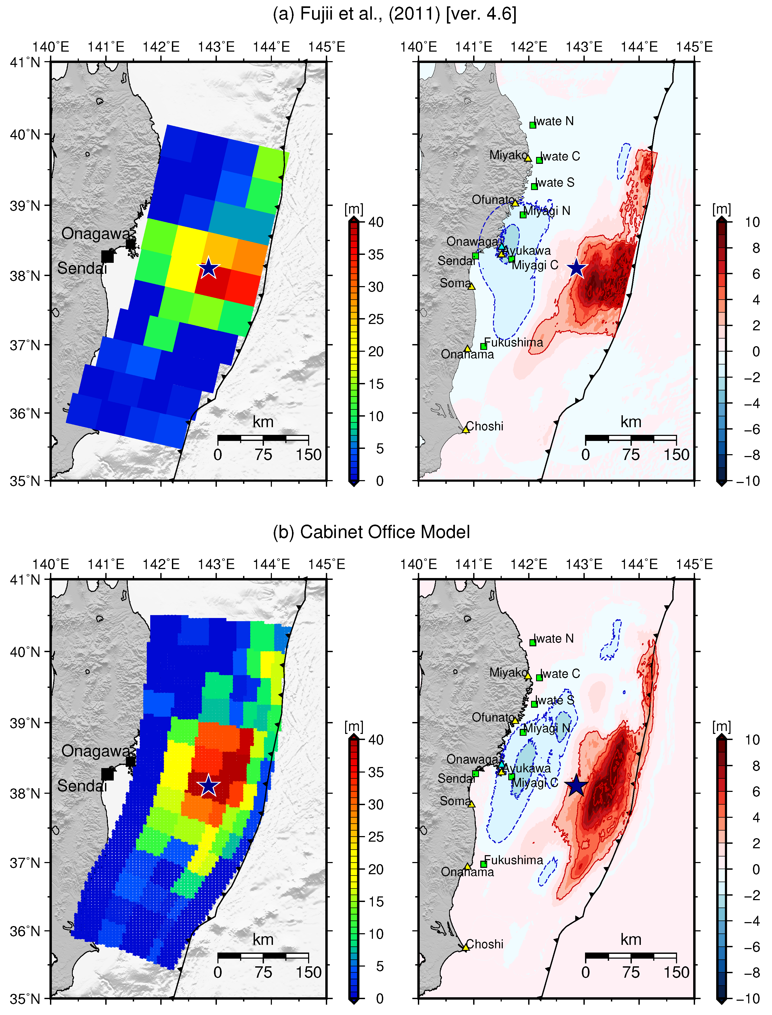
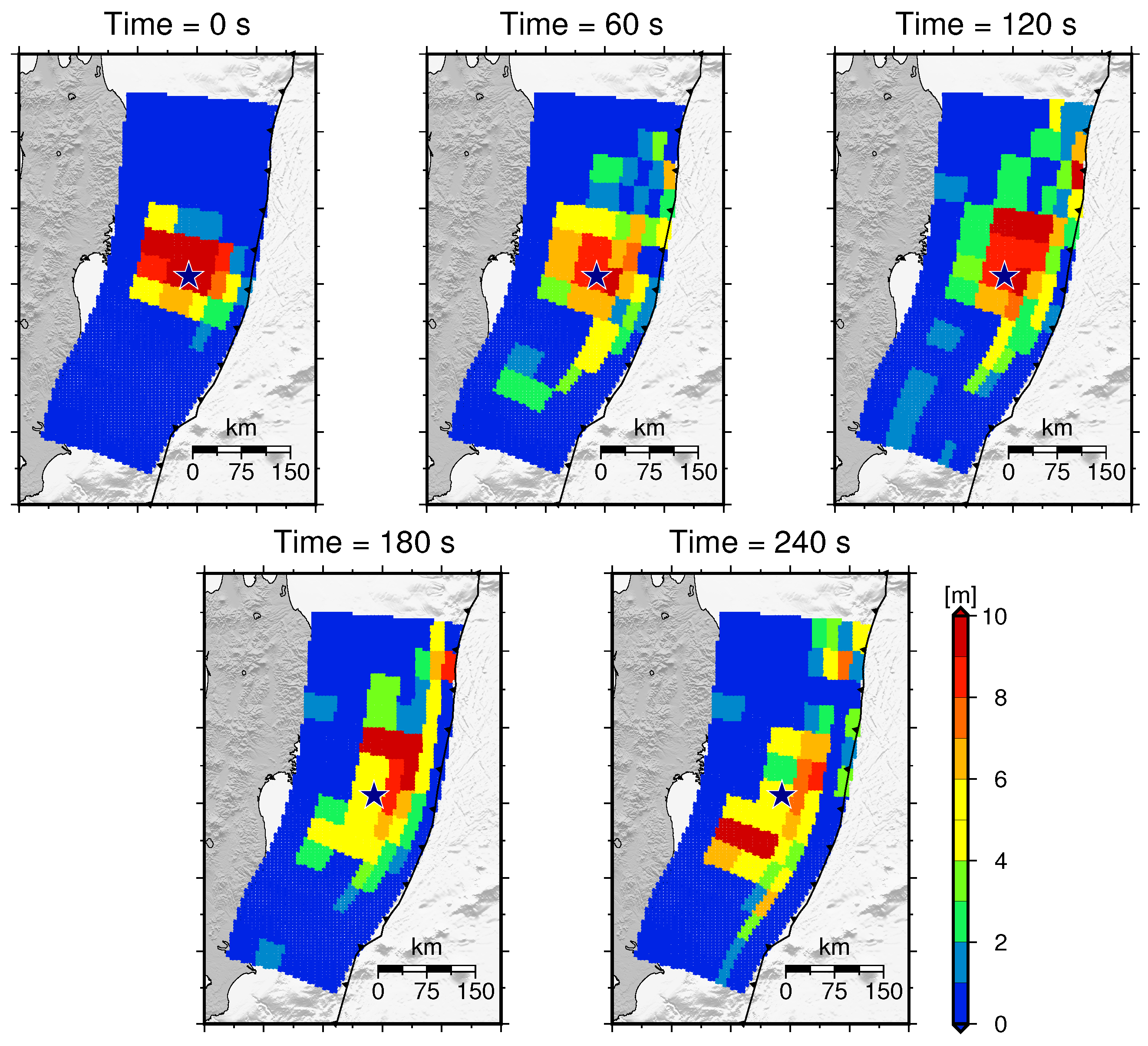
Here, we evaluate two different tsunami source models that were proposed for the 2011 Tohoku tsunami. Model A is a non-uniform slip fault model that is calculated by inverting the tsunami waveforms recorded at several coastal tide gauge stations, offshore pressure gauges, and deep ocean buoy stations. We utilize version 4.6 of the tsunami source model estimated by Fujii et al. [1] (http://iisee.kenken.go.jp/staff/fujii/OffTohokuPacific2011/tsunami_inv_ver4.2and4.6.html). The estimated fault area was 500 km × 200 km and was divided into 40 segments (Figure 1a). The maximum slip was 15.9 m in the shallowest segments near the epicentre. Figure 1a (right) also shows the coseismic deformation calculated from the non-uniform model. The maximum subsidence and uplift displacements were of 2.6 m and 19.1 m, respectively. The maximum deformation was located near the epicentre at the centre-west region of the fault area. Model B corresponds to the earthquake source proposed by the Cabinet Office of Japan [9]. This source was calculated by a joint inversion of geodetic and tsunami data. The slip distribution of this model is characterized by 4575 segments that measure 5 km × 5 km in size. Figure 1b (left) shows the total slip distribution of the estimated fault area. The maximum slip was 27.5 m and was located near the epicentre. Due to the high frequency of high-quality waveform sampling in the available data for the 2011 Tohoku tsunami, this model presents a spatio-temporal slip distribution every 60 s within the first 5 min after the main shock as shown in Figure 2). Figure 1b (right) also shows the coseismic deformation calculated from the total slip amount. This model also generates uplift and deformation regions near the epicentre. The uplift was approximately 12.5 m at the highest point, and the subsidence was approximately 3.6 m at the lowest point.
3. Method
3.1. Tsunami Numerical Simulation
We analyse the capability of each tsunami source model to reproduce the recorded inundation features by conducting tsunami simulations using high-resolution bathymetry data. We employ the Tohoku University’s Numerical Analysis Model for Investigation of Near-field Tsunamis No. 2 (TUNAMI-N2) code. This algorithm solves shallow water equations using a Cartesian coordinate system. The code was developed by the Disaster Control Research Center (DCRC), Tohoku University, Japan [20]. For this study, we revised the run-up modelling conditions by adopting a composite roughness coefficient for the land resistance. We set an equivalent roughness coefficient according to the land use condition [21]. This roughness coefficient considers a building occupancy ratio given by the relation of built-up area in a computational grid [18].
To compute the initial tsunami condition, we assume an instantaneous displacement of the sea surface that is assumed to be identical to the coseismic displacement. The rectangular fault model proposed by [22] is used to calculate the seafloor deformation. We also include the effect of horizontal crustal movement on the total vertical component [23]. The coseismic deformation computed from each spatio-temporal slip distribution (Figure 3) is incorporated into the tsunami propagation model by adding the associated sea surface displacement to the current water surface elevation [18].
3.2. Validation of Source Models
To validate the numerical results calculated from the non-uniform model and the spatio-temporal slip model, we conducted two types of verifications. The first is a comparison of the synthetic and recorded tsunami waveforms from the coastal and offshore tide gauge stations. For this purpose, we calculate the normalized root-mean-square (NRMS) misfit coefficient [24]. This coefficient gives the best agreement between the observed and computed tsunami waveforms for values equal to zero. We use the available tsunami signals of the first wave cycle to compute the NRMS misfit coefficient. The time range of the data used from each station includes the two initial wave cycles (grey bars in Figure 4). However, some coastal stations (Miyako, Ofunato, Ayukawa, Onagawa, Sendai, and Soma) were damaged during the tsunami attack [25]. As a result, these stations only recorded portion of the first tsunami wave. For these stations, we only use the recorded data for the calculation of the NRMS misfit coefficient. The second verification scheme corresponds to the calculated inundation depth in each target area. Here, we calculate the K- and -coefficients proposed by Aida [26]. The first coefficient represents the geometric average of the ratio between the synthetic and observed data. The second coefficient is the fluctuation in the K-coefficient for each observed point. The JSCE guidelines for tsunami assessment of a nuclear power plant [27] recommend that the K-coefficient should be between 0.95 and 1.05, and that the -coefficient should be greater than 1.45.
4. Results and Discussion
4.1. Tsunami Propagation
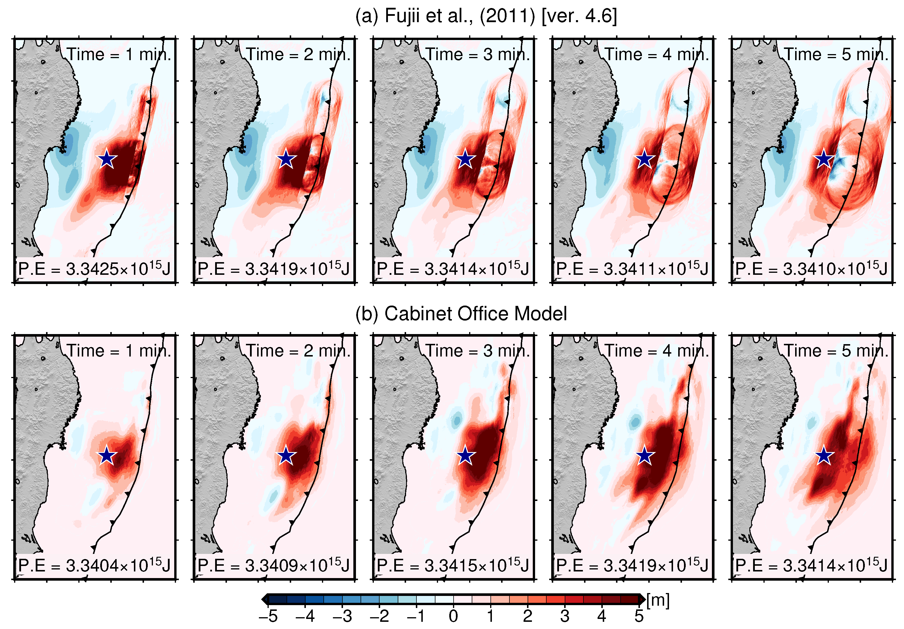
Typically, tsunamis begin to propagate with a single, initial sea surface displacement condition. This initial condition is calculated based on a slip distribution model that defines the rupture area. Tsunami waves then propagate away from the source with a phase velocity depending directly on the local bathymetry [28]. As a result, tsunami inundation features are mainly a function of the initial condition and the local bathymetry. However, the new spatio-temporal slip model for the 2011 Tohoku earthquake incorporates additional coseismic deformation data for the first 5 min of tsunami propagation (at a 60 s interval). At a given propagation time, these additional deformation data are used to update the current sea surface deformation. Figure 3 shows a comparison of five snapshots between the tsunami propagation using both models. The propagation from model A follows a known pattern; the initial condition starts to spread while reducing its wave amplitude (Figure 3a). Conversely, tsunami propagation derived from model B (i.e., the spatio-temporal slip distribution) shows increasing wave amplitudes during the first 4 min of propagation. This fact is verified by the associated tsunami’s potential energy [29]. In the case of the first slip model, the potential energy decreases by approximately 5 × 10 J after each minute of tsunami propagation. Meanwhile, the tsunami’s potential energy associated with the spatio-temporal slip model increases by approximately the same amount of energy.
4.2. Synthetic Tsunami Waveforms
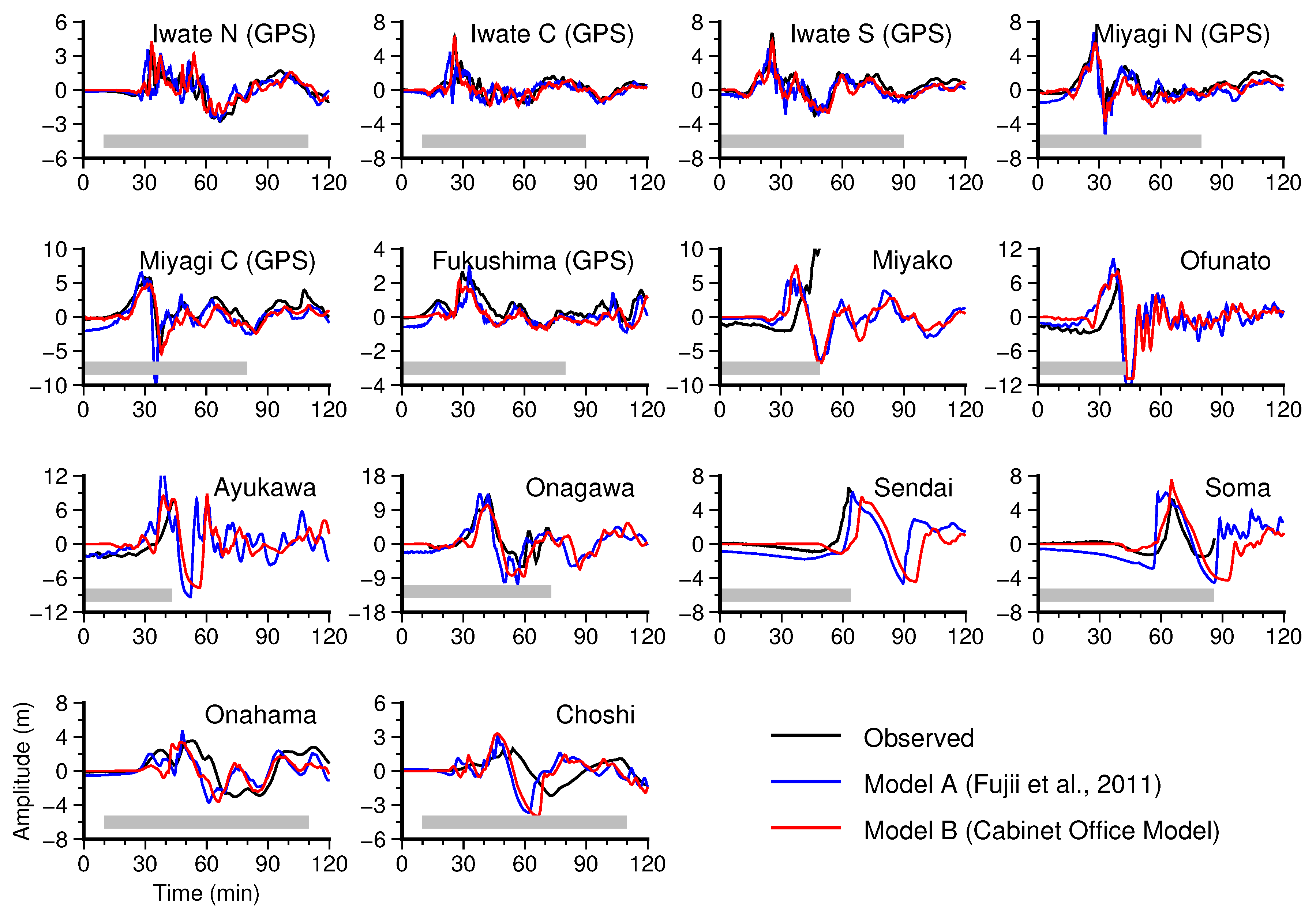
The propagation characteristics described in the previous section will have considerable effects on the arrival time and wave height of the computed tsunami waveform. Figure 4 shows the synthetic tsunami waveforms calculated using both slip models. As expected, the shallow water equations are capable of adequately solving the first and later phase components of the tsunami waveforms at the locations of the offshore GPS buoys stations (Iwate North, Iwate Central, Iwate South). There are, however, some discrepancies in the initial wave amplitude. While the computed initial amplitude using model B at the Miyagi Central and Miyagi North stations is consistent with the recorded one (approximately −50 cm), the computed amplitude using model A is approximately −2 m. This condition is also observed at the Ofunato station (Figure 4). This difference is likely due to the initial sea surface deformation that generated the lowest subsidence near the location of the coastal stations.
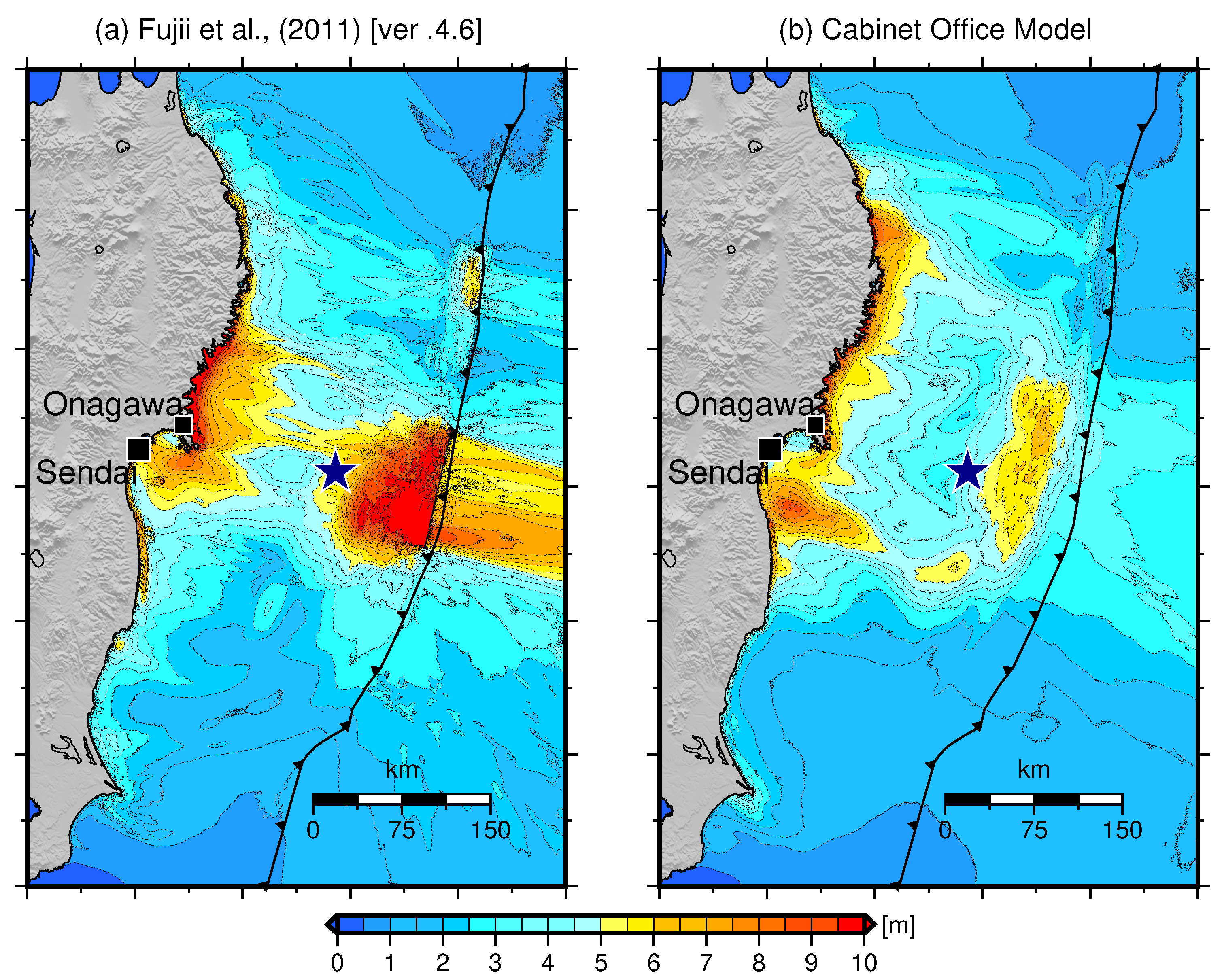
Meanwhile, there are apparent differences in the synthetic waveforms computed at the coastal stations, where the tsunami propagation mainly follows a nonlinear behaviour due to shallow bathymetry and coastal morphology. For instance, the maximum tsunami amplitude estimated at the Ofunato, Ayukawa, and Onagawa stations using model A is slightly higher than the recorded amplitude. Furthermore, in case of Onagawa station, two peaks characterize its maximum amplitude (Figure 4). Although nonlinear effects due to shallow bathymetry may contribute to the waveform shape at this location, this double peak does not appear in the synthetic waveform calculated at the same location using the second slip model. In the case of the Sendai station, only half of the initial waveform data are available due to the destruction of the tide gauge at this location. The initial computed amplitudes using both models at this station display similar characteristics to those calculated at the Ofunato, Ayukawa, and Onagawa stations (Figure 4). At the Sendai station, the tsunami propagation from model A better reproduces the observed small amplitude (Figure 4b). Concerning the arrival time, however, model A shows better reproducibility than model B. In the case of model B, the tsunami wave arrives approximately 10 min late. The maximum tsunami height estimated from each slip model is shown in Figure 5. In general, each model generates the maximum height along the coast of Sanriku to the north of the Tohoku region (Figure 5). The tsunami height around the Sendai Plain, however, is the highest in the case of model B (Figure 5b). These different features of the synthetic tsunami waveforms and the maximum tsunami height further define the effects of the spatio-temporal slip distribution on modelling the tsunami inundation.
To determine the slip model that provides the best fit for the recorded tsunami waveforms, we calculate the normalized root-mean-square (NRMS) misfit coefficient [24]. First, we calculate the NRMS misfit using only the offshore GPS stations. The coefficients are 0.35 and 0.25 for model A and model B, respectively. Regarding the tsunami waveform at coastal stations, the NRMS is 0.77 and 0.65 for model A and model B, respectively. These values indicate that model B can fit the observed data with an approximately 30% better accuracy relative to the first slip model.
4.3. Inundation Depths
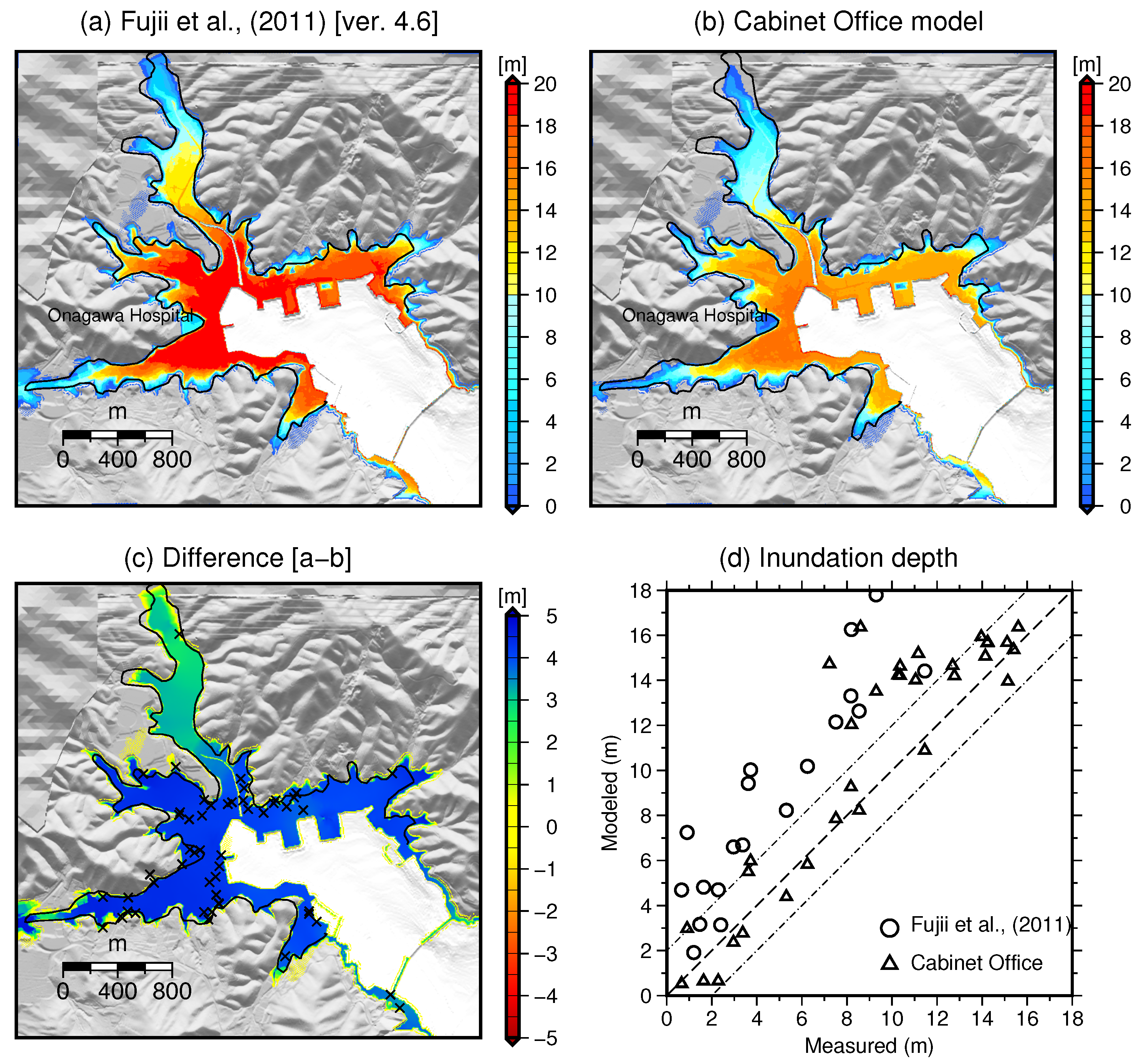
In the case of Onagawa, our calculations suggest that the tsunami arrived approximately 30 min after the main shock. Topographic features mainly constrain the estimated inundation areas. In general, the inundation limits are consistent with those estimated by the GSI (Figure 6a,b). The local flow depth within the inundated area, however, shows very different outcomes. In most of the flooded area, the maximum inundation depth estimated using model A is approximately 5 m higher than the calculated maximum depth using model B (Figure 6c). For instance, the measured inundation depth at Onagawa Hospital was 1.95 m [18]; at this same location, model A estimates an inundation depth of approximately 6 m. Model B, however, estimates an inundation depth of approximately 2 m. A point-to-point comparison of the modelled and measured tsunami inundation depths (Figure 6d) further illustrates the overestimation of the measured data by the results using model A. Therefore, to test the reproducibility of each slip model, we calculate the Aida parameters (Table 1). Based on the K- and -coefficients, the inundation results from the second slip model better reproduce the local inundation depths in Onagawa.
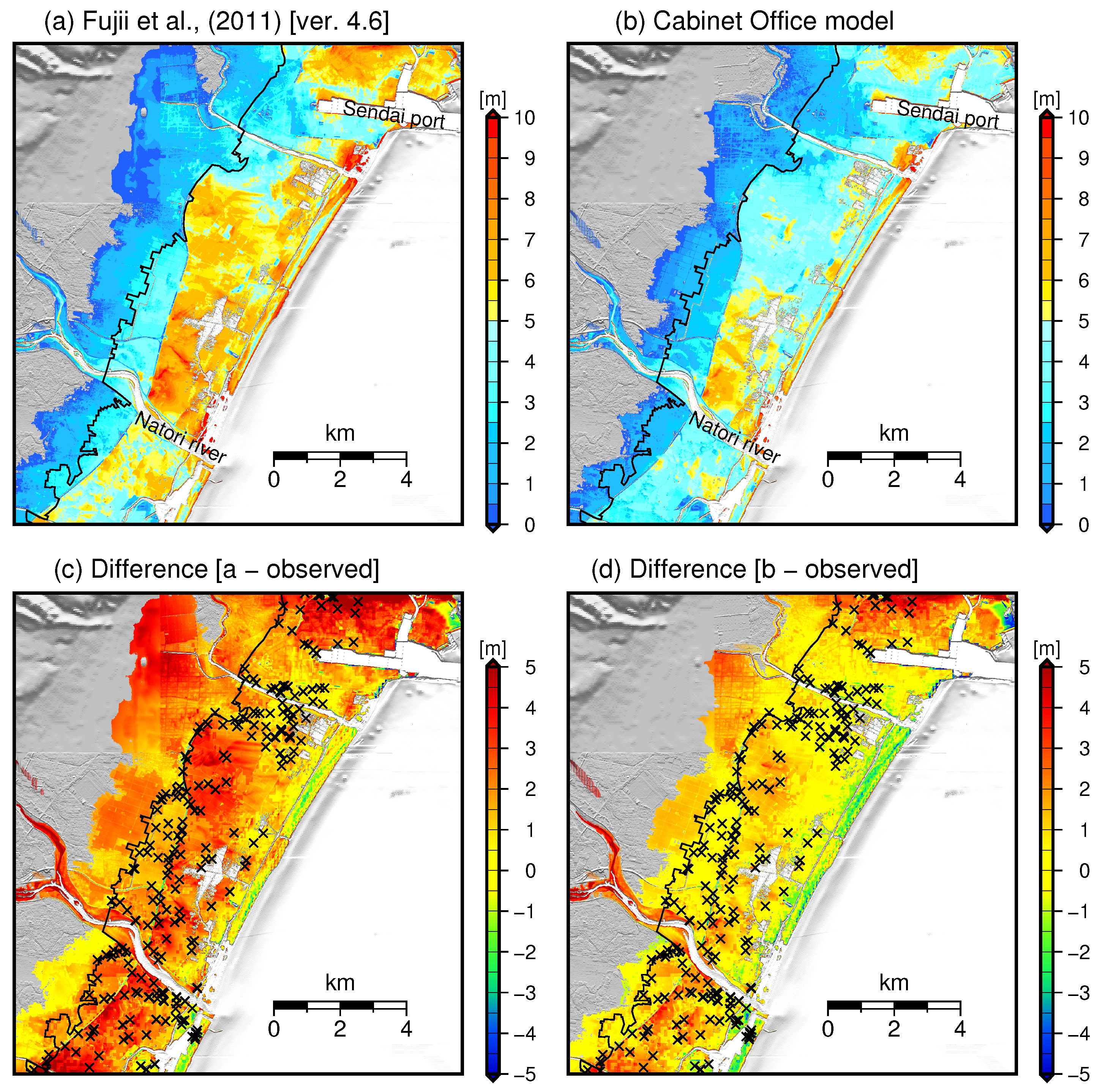
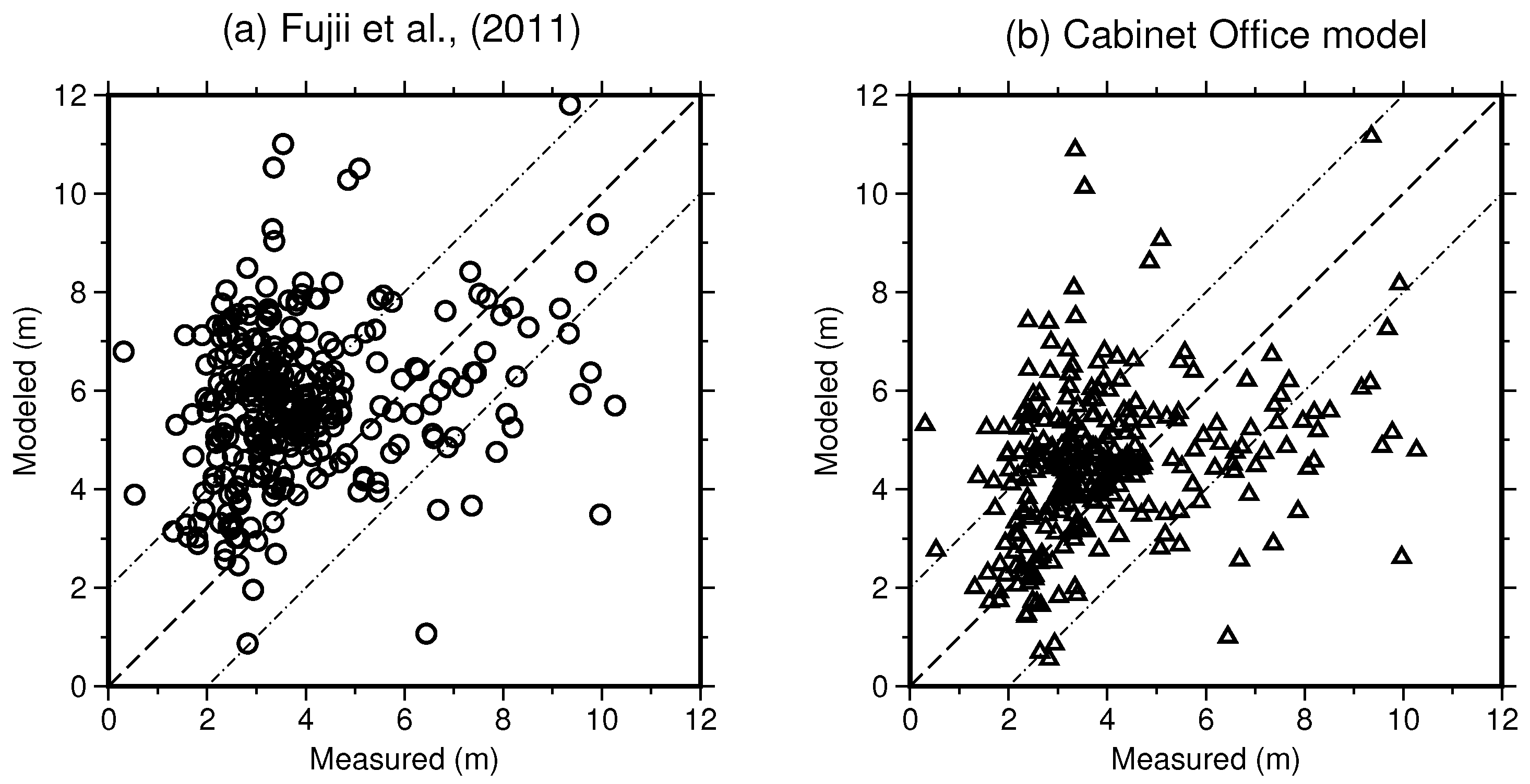
The inundation area in the Sendai Plain determined from both slip models exceeds the estimated inundation limits from the GSI. In this area, unlike Onagawa, the flooded areas were mainly characterized by the tsunami source and local bathymetry rather than the topographic features (Figure 7a,b). Figure 7c,d are calculated by subtracting the measured inundation depth (GSI) from the inundation result estimated by each slip model. The local inundation depths in the inundation zone show smaller differences between both models. The maximum difference can be found near the coastline and to the north of the Natori River. In general, both slip models overestimate the measured data. Near the coastline, however, both models are approximately 1 m lower than measured inundation depth. Although the differences in the inundation depths for the Sendai Plain are generally of 2 m, the results also show that, as observed for Onagawa, model A generates more significant inundation run-up relative to model B. A point-to-point comparison of the modelled and measured tsunami inundation depths (Figure 8) shows that neither slip model can fully replicate the measured data. In general, both models produce higher flood depths. Nevertheless, to test the reproducibility of each slip model, we also calculate the Aida parameters (Table 1) in this target area. Based on the K- and -coefficients, the inundation results from model B still show better agreement concerning the replicated measured inundation depths.
5. Conclusions
We analysed a new spatio-temporal slip model for the 2011 Tohoku earthquake and tsunami to reproduce the observed inundation depths at two locations in the affected area. The spatio-temporal slip model (model B) was compared against a non-uniform slip model (model A). For model B, we adopted the earthquake source proposed by the Cabinet Office of Japan [9]. Model A is based on the tsunami data-inferred slip model estimated by Fujii et al. [1] (version 4.6). Our results revealed that model B better replicated the observed data. Regarding the tsunami waveforms recorded at the coastal tide gauge station and the offshore stations, the new proposed slip distribution showed an approximately 30% better accuracy relative to slip model A. Furthermore, by comparing the local inundation features at the two different locations with unique topographic and coastal morphological characteristics, we found that the Cabinet Office model also better replicated the measured inundation depths. Finally, our numerical results for the 2011 Tohoku earthquake and tsunami suggested that, while single non-uniform slip models can reasonably solve for tsunami propagation and inundation features, the new spatio-temporal slip model shows great potential for the same task. Thus, considering that tsunami-induced damage directly depends on various inundation features such as the flow depth and flow velocity, the implementation of this model can lead to more realistic damage scenarios.
Acknowledgments
This research was supported by the Japan Society for the Promotion of Science (JSPS) under the Project “Fusion of Real-time Simulation and Remote Sensing for Tsunami Damage Estimation in Latin America” (JSPS-Grant: P16055), and JST CREST (Grant number JPMJCR1411).
Author Contributions
Bruno Adriano made overall design and calculations of the study and drafted the manuscript. Satomi Hayashi preprocessed the initial topography/bathymetry data for the tsunami simulation of Sendai area. Shunichi Koshimura contributed in designing the study. All authors read and approved the final manuscript.
Conflicts of Interest
The authors declare no conflict of interest.
References
- Fujii, Y.; Satake, K.; Sakai, S.; Shinohara, M.; Kanazawa, T. Tsunami source of the 2011 off the Pacific coast of Tohoku Earthquake. Earth Planets Space 2011, 63, 815–820. [Google Scholar] [CrossRef]
- Gusman, A.R.; Tanioka, Y.; Sakai, S.; Tsushima, H. Source model of the great 2011 Tohoku earthquake estimated from tsunami waveforms and crustal deformation data. Earth Planet. Sci. Lett. 2012, 341–344, 234–242. [Google Scholar] [CrossRef]
- Ammon, C.J.; Lay, T.; Kanamori, H.; Cleveland, M. A rupture model of the 2011 off the Pacific coast of Tohoku Earthquake. Earth Planets Space 2011, 63, 693–696. [Google Scholar] [CrossRef]
- Lay, T.; Ammon, C.J.; Kanamori, H.; Kim, M.J.; Xue, L. Outer trench-slope faulting and the 2011 M w 9.0 off the Pacific coast of Tohoku Earthquake. Earth Planets Space 2011, 63, 713–718. [Google Scholar] [CrossRef]
- Satake, K.; Fujii, Y. Review: Source Models of the 2011 Tohoku Earthquake and Long-Term Forecast of Large Earthquakes. J. Disaster Res. 2014, 9, 272–280. [Google Scholar] [CrossRef]
- MacInnes, B.T.; Gusman, A.R.; LeVeque, R.J.; Tanioka, Y. Comparison of earthquake source models for the 2011 Tohoku event using tsunami simulations and near-field observations. Bull. Seismol. Soc. Am. 2013, 103, 1256–1274. [Google Scholar] [CrossRef]
- Ulutas, E. Comparison of the seafloor displacement from uniform and non-uniform slip models on tsunami simulation of the 2011 Tohoku–Oki earthquake. J. Asian Earth Sci. 2013, 62, 568–585. [Google Scholar] [CrossRef]
- Satake, K.; Fujii, Y.; Harada, T.; Namegaya, Y. Time and Space Distribution of Coseismic Slip of the 2011 Tohoku Earthquake as Inferred from Tsunami Waveform Data. Bull. Seismol. Soc. Am. 2013, 103, 1473–1492. [Google Scholar] [CrossRef]
- Massive Earthquake Model Review Meeting of the Nankai Trough; Cabinet Office, Government of Japan: Tokyo, Japan, 2012.
- Gokon, H.; Koshimura, S. Mapping of Building Damage of the 2011 Tohoku Earthquake Tsunami in Miyagi Prefecture. Coast. Eng. J. 2012, 54, 1250006. [Google Scholar] [CrossRef]
- Suppasri, A.; Mas, E.; Charvet, I.; Gunasekera, R.; Imai, K.; Fukutani, Y.; Abe, Y.; Imamura, F. Building damage characteristics based on surveyed data and fragility curves of the 2011 Great East Japan tsunami. Nat. Hazards 2012, 66, 319–341. [Google Scholar] [CrossRef]
- Mikami, T.; Shibayama, T.; Esteban, M.; Matsumaru, R. Field Survey of the 2011 Tohoku Earthquake and Tsunami in Miyagi and Fukushima Prefectures. Coast. Eng. J. 2012, 54, 1250011. [Google Scholar] [CrossRef]
- Latcharote, P.; Suppasri, A.; Yamashita, A.; Adriano, B.; Koshimura, S.; Kai, Y.; Imamura, F. Mechanism and Stability Analysis of Overturned Buildings by the 2011 Great East Japan Earthquake and Tsunami in Onagawa Town. In Proceedings of the 14th Japan Earthquake Engineering Symposium, Chiba, Japan, 4–6 December 2014; pp. 108–117. [Google Scholar]
- Mori, N.; Takahashi, T.; Yasuda, T.; Yanagisawa, H. Survey of 2011 Tohoku earthquake tsunami inundation and run-up. Geophys. Res. Lett. 2011, 38. [Google Scholar] [CrossRef]
- Mori, N.; Takahashi, T.; The 2011 Tohoku Earthquake Tsunami Joint Survey Group. Nationwide post event survey and analysis of the 2011 Tohoku Earthquake Tsunami. Coast. Eng. J. 2012, 54, 1250001. [Google Scholar] [CrossRef]
- Mori, N.; Cox, D.T.; Yasuda, T.; Mase, H. Overview of the 2011 Tohoku Earthquake Tsunami Damage and Its Relation to Coastal Protection along the Sanriku Coast. Earthq. Spectra 2013, 29, S127–S143. [Google Scholar] [CrossRef]
- Koshimura, S.; Hayashi, S.; Gokon, H. Lessons from the 2011 Tohoku Earthquake Tsunami Disaster. J. Disaster Res. 2013, 8, 549–560. [Google Scholar] [CrossRef]
- Adriano, B.; Hayashi, S.; Gokon, H.; Mas, E.; Koshimura, S. Understanding the Extreme Tsunami Inundation in Onagawa Town by the 2011 Tohoku Earthquake, Its Effects in Urban Structures and Coastal Facilities. Coast. Eng. J. 2016, 58, 1640013. [Google Scholar] [CrossRef]
- Hayashi, S.; Koshimura, S. The 2011 Tohoku Tsunami Flow Velocity Estimation by the Aerial Video Analysis and Numerical Modeling. J. Disaster Res. 2013, 8, 561–572. [Google Scholar] [CrossRef]
- Imamura, F. Review of the tsunami simulation with a finite difference method. In Long Wave Run-up Models; Yeh, H., Liu, P., Synolakis, C., Eds.; World Scientific: Singapore, 1996; pp. 25–42. [Google Scholar]
- Imai, K.; Imamura, F.; Iwama, S. Advanced Tsunami Computation for Urban Regions. J. Jpn. Soc. Civ. Eng. 2013, 69, 311–315. [Google Scholar] [CrossRef]
- Okada, Y. Surface deformation due to shear and tensile faults in a half-space. Bull. Seismol. Soc. Am. 1985, 75, 1135–1154. [Google Scholar]
- Tanioka, Y.; Satake, K. Tsunami generation by horizontal displacement of ocean bottom. Geophys. Res. Lett. 1996, 23, 861. [Google Scholar] [CrossRef]
- Heidarzadeh, M.; Murotani, S.; Satake, K.; Ishibe, T.; Gusman, A.R. Source model of the 16 September 2015 Illapel, Chile, M w 8.4 earthquake based on teleseismic and tsunami data. Geophys. Res. Lett. 2016, 43, 643–650. [Google Scholar] [CrossRef]
- Suppasri, A.; Koshimura, S.; Imai, K.; Mas, E.; Gokon, H.; Muhari, A.; Imamura, F. Damage Characteristic and Field Survey of the 2011 Great East Japan Tsunami in Miyagi Prefecture. Coast. Eng. J. 2012, 54, 1250005. [Google Scholar] [CrossRef]
- Aida, I. Reliability of a tsunami source model derived from fault parameters. J. Phys. Earth 1978, 26, 57–73. [Google Scholar] [CrossRef]
- Tsunami Assessment Method for Nuclear Power Plants in Japan, Japan Society of Civil Engineers. Available online: https://www.jsce.or.jp/committee/ceofnp/Tsunami/eng/JSCE_Tsunami_060519.pdf (accessed on 22 December 2017).
- Satake, K. Linear and nonlinear computations of the 1992 Nicaragua earthquake tsunami. Pure Appl. Geophys. PAGEOPH 1995, 144, 455–470. [Google Scholar] [CrossRef]
- Satake, K.; Tanioka, Y. The July 1998 Papua New Guinea Earthquake: Mechanism and Quantification of Unusual Tsunami Generation. Pure Appl. Geophys. 2003, 160, 2087–2118. [Google Scholar] [CrossRef]
Figure 1.
(a) Fault slip distribution and corresponding coseismic displacement was calculated using model A (Fujii et al. [1]). The blue star indicates the location of the epicentre as per the Japan Meteorological Agency (JMA). The black rectangles show the target areas used for the tsunami inundation modelling. (b) Total slip distribution and corresponding coseismic displacement was calculated using earthquake source model B ([9]). The triangles and squares indicate the location of the coastal tide gauge and offshore GPS wave gauge stations, respectively. Colours indicate the operating agencies (Green: the Nationwide Ocean Wave Information Network for Ports and HArbourS (NOWPHAS) of Japan; yellow: Japan Meteorological Agency (JMA); and light blue: the Onagawa Nuclear Power Plant of the Tohoku Electric Power Company of Japan). The contour lines in the left panels are drawn at 1-m intervals.

Figure 2.
Spatio-temporal slip distribution of the earthquake source proposed by the Cabinet Office of Japan [9]. The blue star indicates the epicentre (JMA).
Figure 2.
Spatio-temporal slip distribution of the earthquake source proposed by the Cabinet Office of Japan [9]. The blue star indicates the epicentre (JMA).

Figure 3.
Snapshots at 1, 2, 3, 4, and 5 min of tsunami propagation. (a) Snapshots calculated from the tsunami source model proposed by Fujii et al. [1]; (b) Snapshots calculated using the spatio-temporal earthquake slip distribution proposed by the Cabinet Office of Japan [9]. The blue star indicates the location of the epicentre.

Figure 4.
Comparison of recorded (black line) and computed tsunami waveforms as per Fujii et al. [1] (blue line) and the Cabinet Office [9] (red line). The grey bars indicate the time frames used to compute the normalized root-mean-square (NRMS) misfit coefficients.

Figure 5.
(a) Maximum tsunami heights computed using the tsunami source proposed by Fujii et al. [1] (model A). (b) Maximum tsunami heights estimated using the spatio-temporal earthquake source from the Cabinet Office Model [9] (model B).

Figure 6.
Onagawa computational area. (a) Maximum inundation depth computed using the tsunami source published by Fujii et al. [1]; (b) Maximum inundation depth estimated using the earthquake source developed by the Cabinet Office of Japan (Cabinet Office 2012); (c) Difference in the maximum inundation depth between the Fujii et al. [1] and the Cabinet Office [9] models. The x symbols show the locations of the Japan Society of Civil Engineers (JSCE) measurements. The black line indicates the inundation limits estimated by the Geospatial Information Authority of Japan (GSI); (d) Comparison between the JSCE field survey data and the computed inundation depths. The triangles and circles show the computed inundation depths using the Fujii et al. [1] model and the Cabinet Office [1] model, respectively.

Figure 7.
Sendai computational area. (a) Maximum inundation depth computed using the tsunami source published by Fujii et al. [1]; (b) Maximum inundation depth estimated using the earthquake source developed by the Cabinet Office of Japan ([9]); (c) The difference in the maximum inundation depth between the Fujii et al. [1] model and measured inundation depth; (d) The difference in the maximum inundation depth between the Cabinet Office [9] model and measured inundation depth. The x symbols show the locations of the JSCE measurements. The black line indicates the inundation limits estimated by the GSI.

Figure 8.
Comparison between the JSCE field survey data and the computed inundation depth from the Fujii et al. [1] (a) and Cabinet Office [9]; (b) models.


Table 1.
Aida parameters calculated from both source model for each target area.
| Model | Onagawa | Sendai | ||
|---|---|---|---|---|
| K | K | |||
| Fujii et al. [1] | 0.45 | 1.11 | 0.58 | 1.11 |
| Cabinet Office model | 0.90 | 1.15 | 0.77 | 1.12 |
© 2017 by the authors. Licensee MDPI, Basel, Switzerland. This article is an open access article distributed under the terms and conditions of the Creative Commons Attribution (CC BY) license (http://creativecommons.org/licenses/by/4.0/).
Share and Cite
MDPI and ACS Style
Adriano, B.; Hayashi, S.; Koshimura, S. Analysis of Spatio-Temporal Tsunami Source Models for Reproducing Tsunami Inundation Features. Geosciences 2018, 8, 3. https://doi.org/10.3390/geosciences8010003
AMA Style
Adriano B, Hayashi S, Koshimura S. Analysis of Spatio-Temporal Tsunami Source Models for Reproducing Tsunami Inundation Features. Geosciences. 2018; 8(1):3. https://doi.org/10.3390/geosciences8010003
Chicago/Turabian StyleAdriano, Bruno, Satomi Hayashi, and Shunichi Koshimura. 2018. "Analysis of Spatio-Temporal Tsunami Source Models for Reproducing Tsunami Inundation Features" Geosciences 8, no. 1: 3. https://doi.org/10.3390/geosciences8010003
Note that from the first issue of 2016, this journal uses article numbers instead of page numbers. See further details here.