Optical Remote Sensing Potentials for Looting Detection


Abstract
:1. Introduction
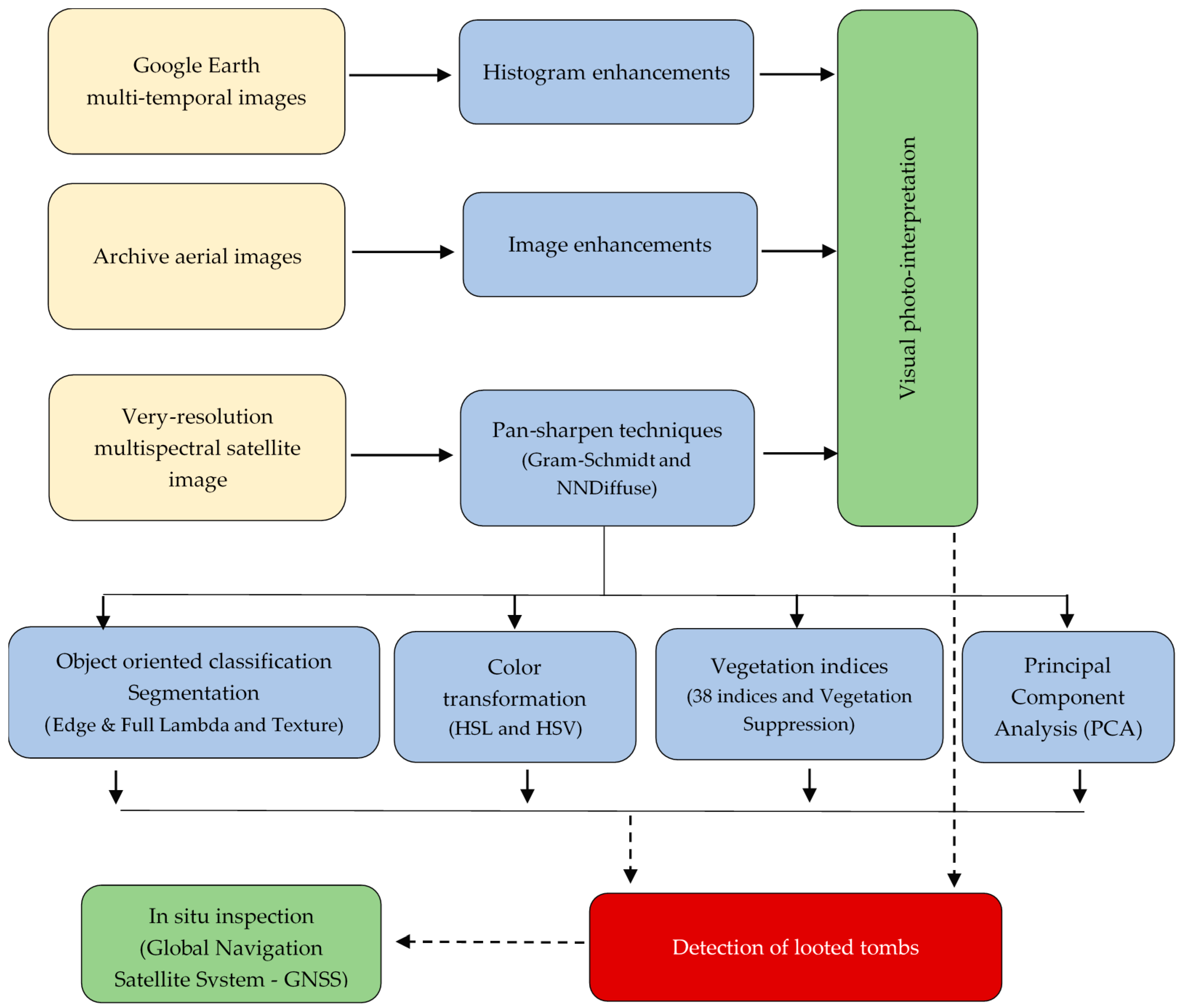
2. Methodology
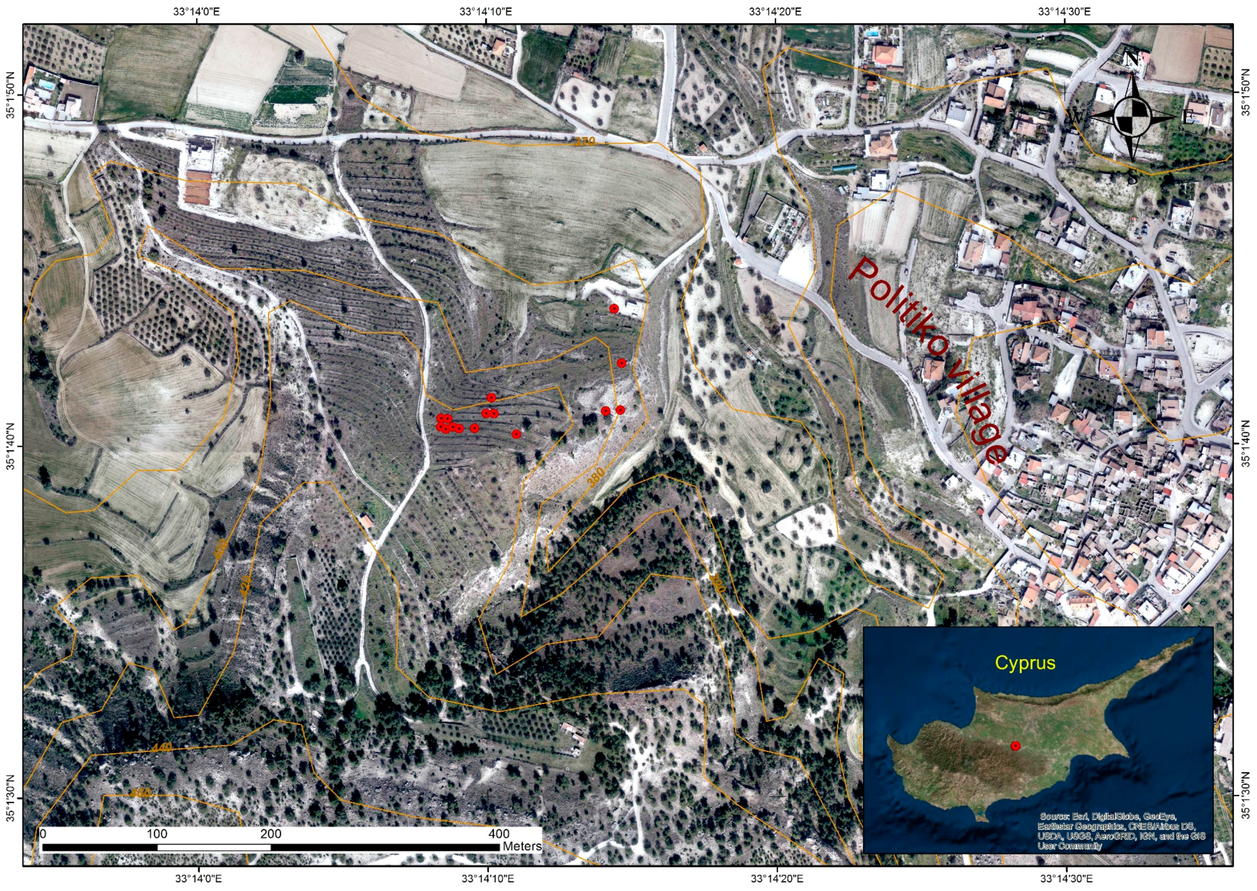
3. Case Study Area
4. Results
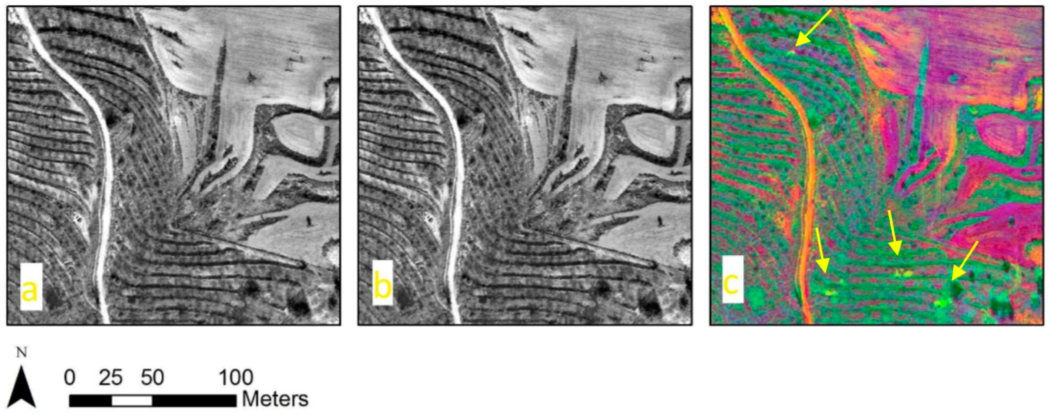
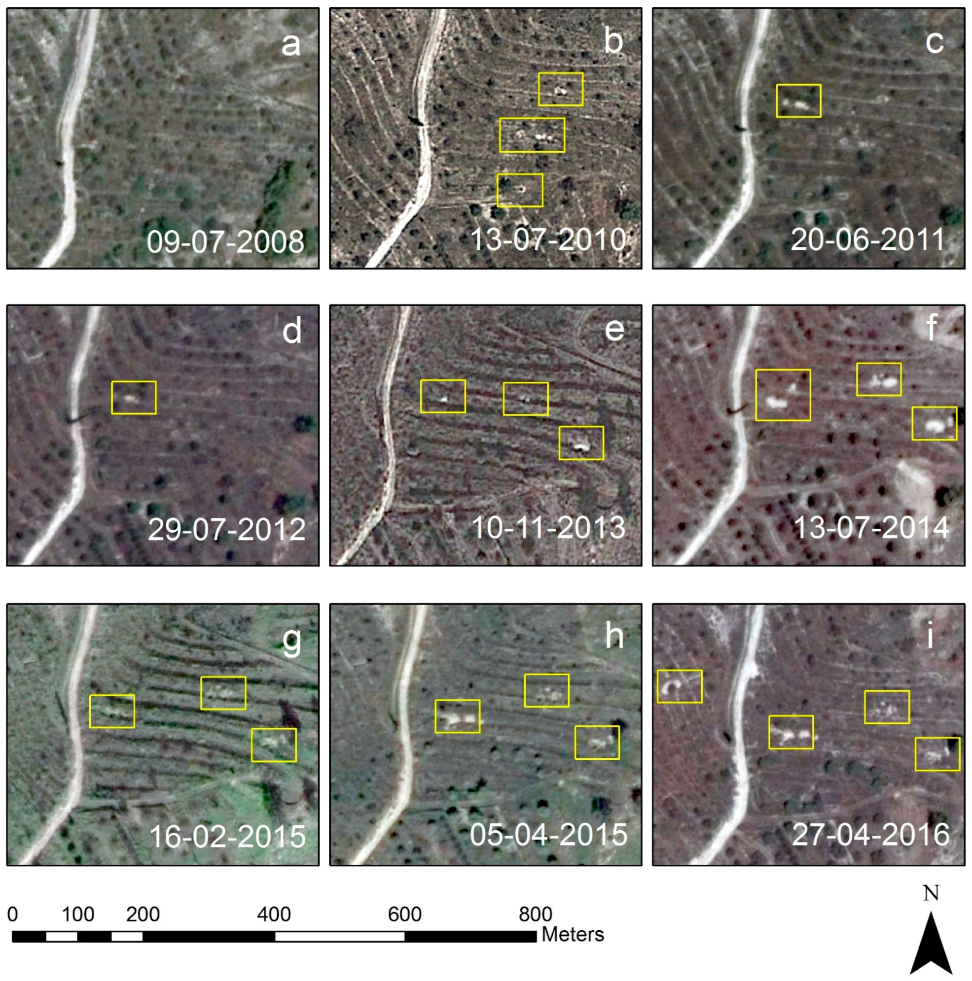
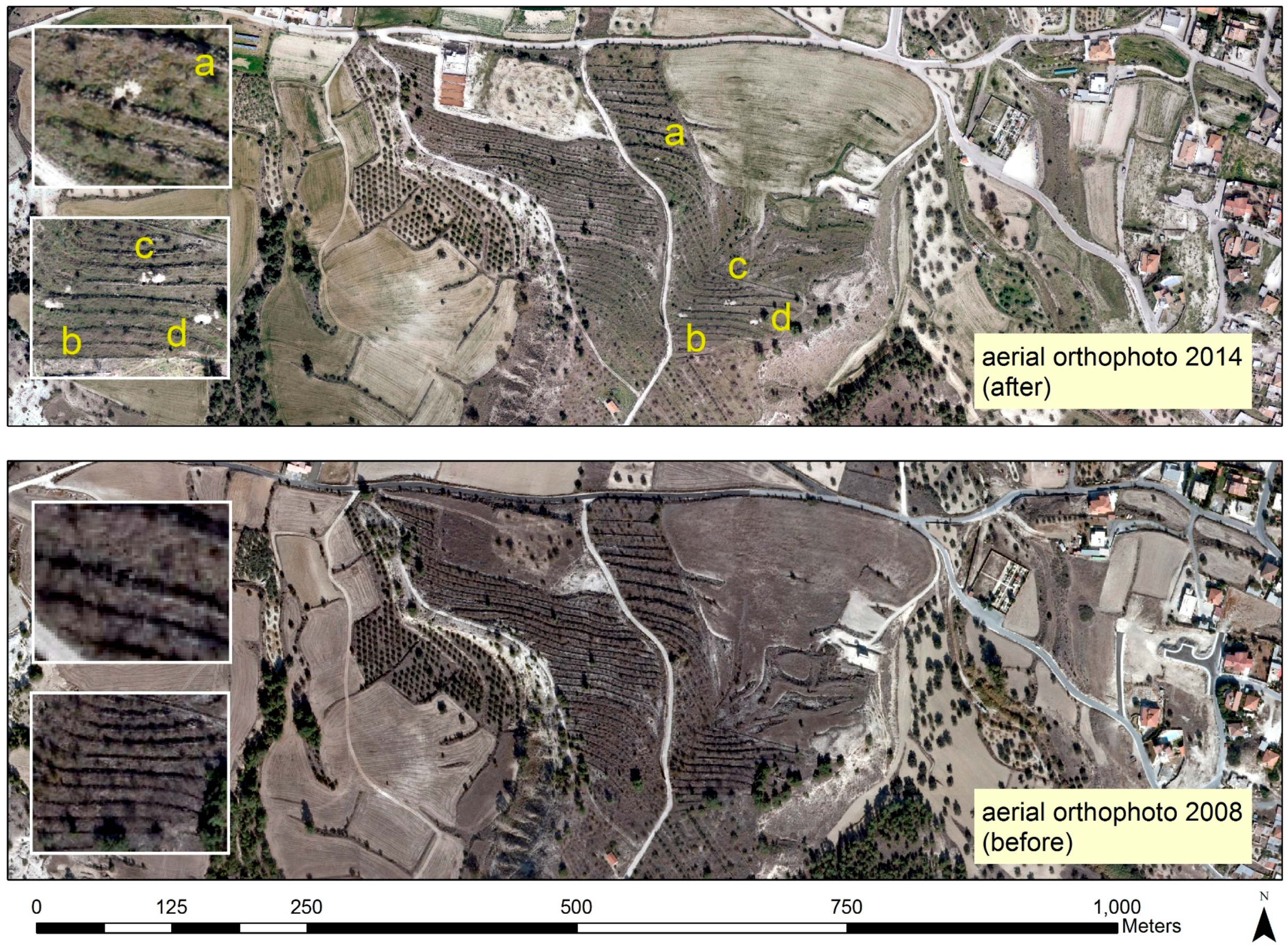
4.1. Aerial Orthophotos and Google Earth© Images
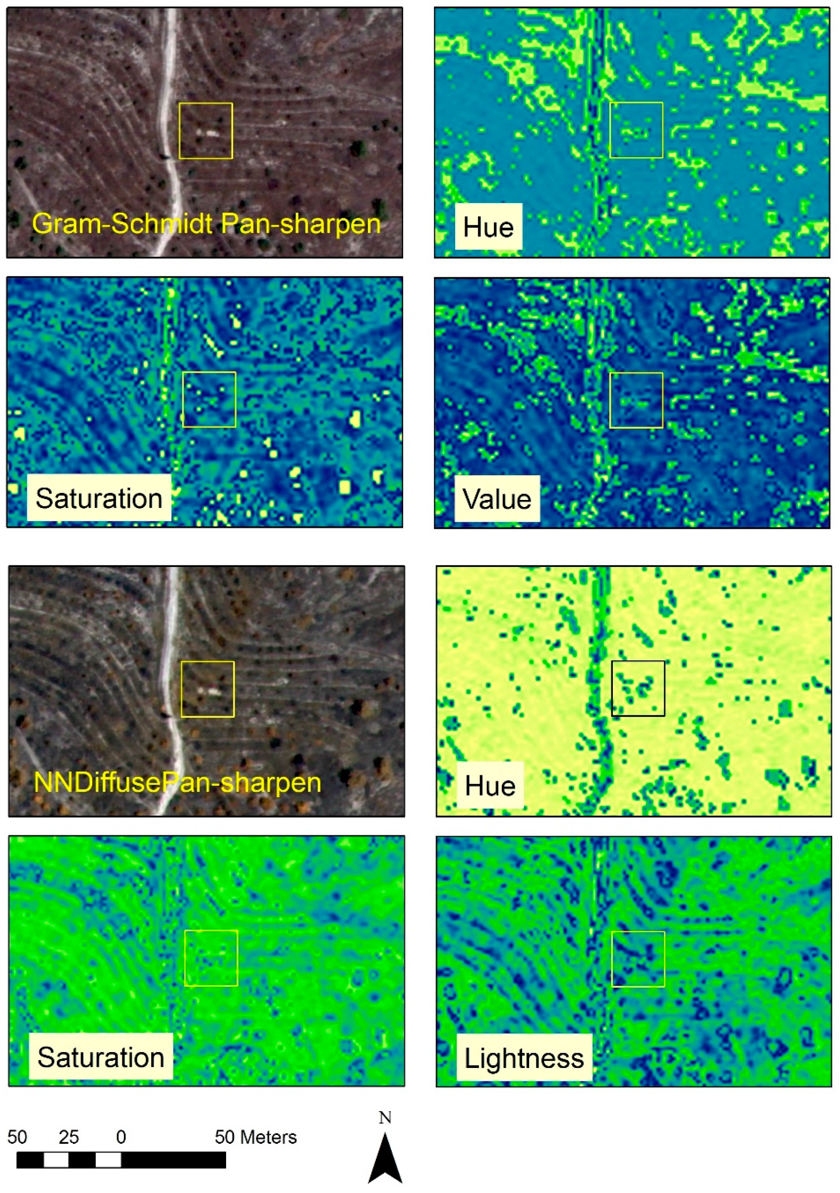
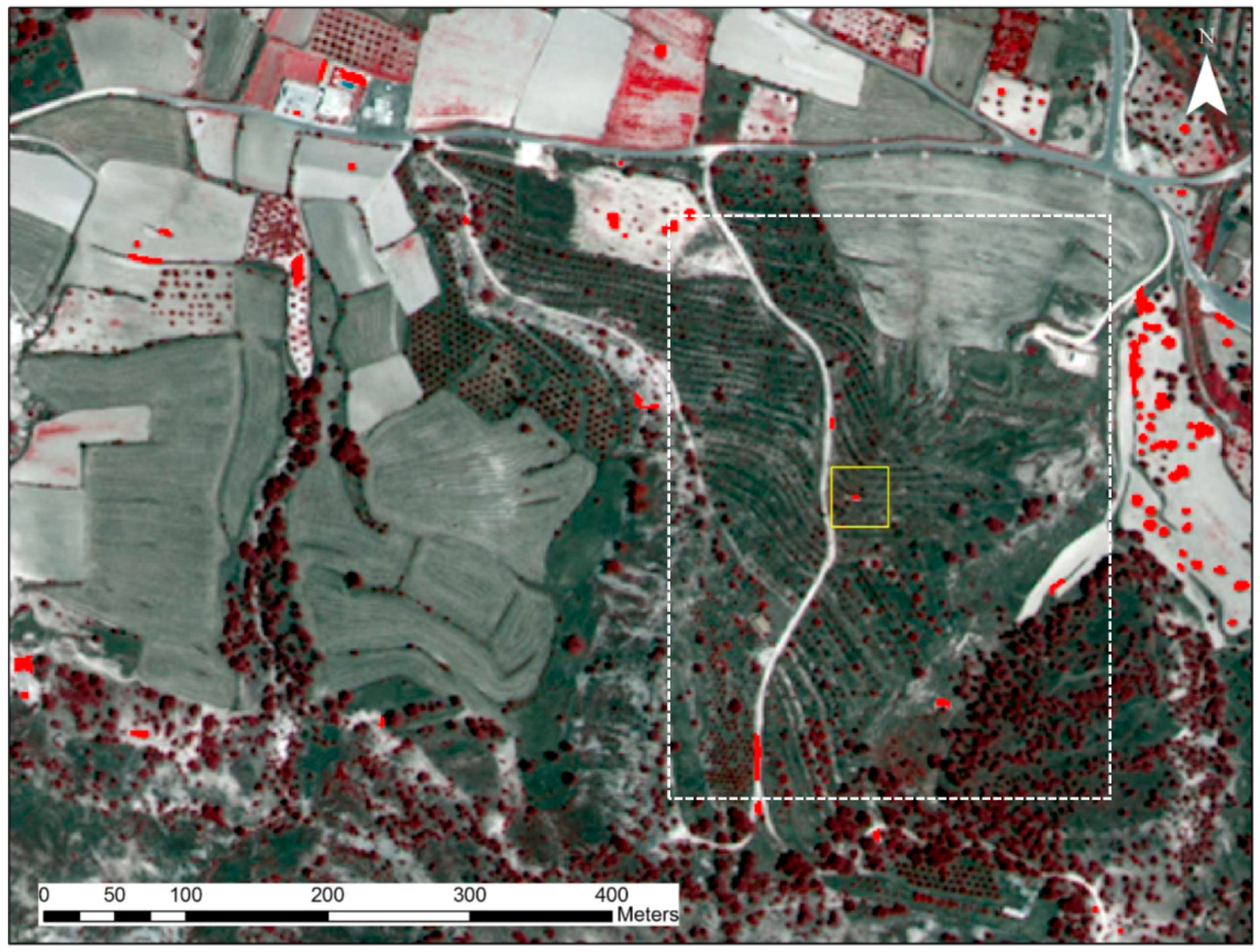
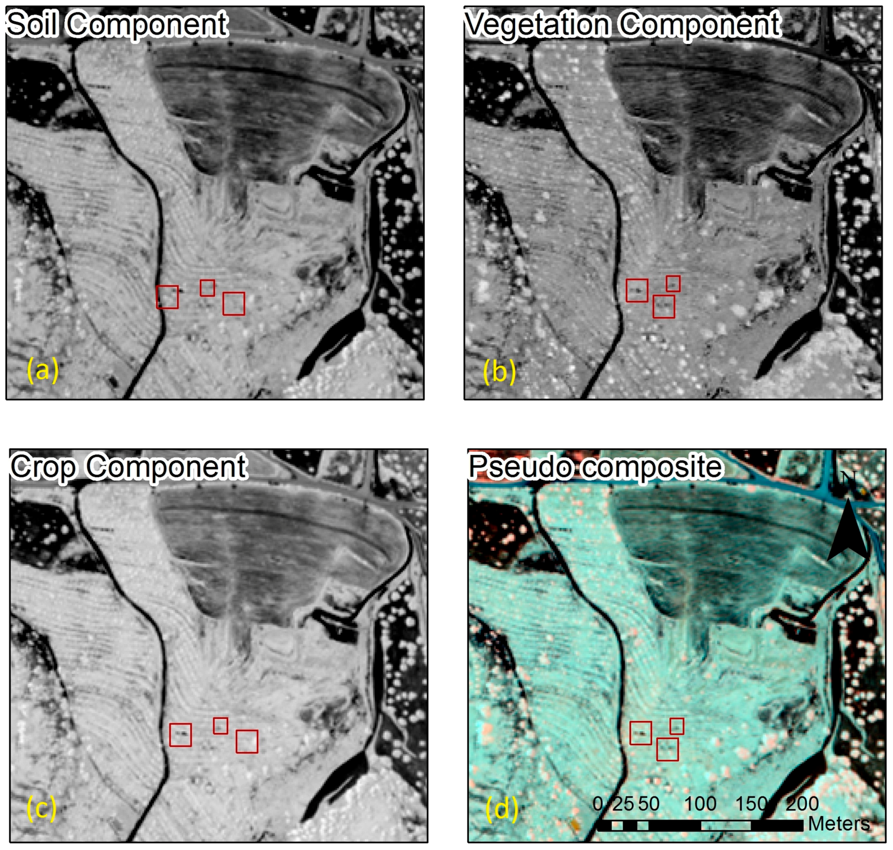
4.2. Satellite Image Processing
- is region i of the image,
- is the area of region i,
- is the average value in region i,
- is the average value in region j,
- is the Euclidean distance between the spectral values of regions i and j,
- is the length of the common boundary of and .
5. Conclusions
Acknowledgments
Author Contributions
Conflicts of Interest
References
- Convention on the Means of Prohibiting and Preventing the Illicit Import, Export and Transfer of Ownership of Cultural Property; UNESCO: Paris, France, 1970.
- UNIDROIT. Convention on Stolen or Illegally Exported Cultural Objects; UNIDROIT: Rome, Italy, 1995. [Google Scholar]
- Tapete, D.; Cigna, F.; Donoghue, N.M.D. ‘Looting marks’ in space-borne SAR imagery: Measuring rates of archaeological looting in Apamea (Syria) with TerraSAR-X Staring Spotlight. Remote Sens. Environ. 2016, 178, 42–58. [Google Scholar] [CrossRef]
- Chase, F.A.; Chase, Z.D.; Weishampel, F.J.; Drake, B.J.; Shrestha, L.R.; Slatton, L.C.; Awe, J.J.; Carter, E.W. Airborne LiDAR, archaeology, and the ancient Maya landscape at Caracol, Belize. J. Archaeol. Sci. 2011, 38, 387–398. [Google Scholar] [CrossRef]
- Lasaponara, R.; Leucci, G.; Masini, N.; Persico, R. Investigating archaeological looting using satellite images and GEORADAR: The experience in Lambayeque in North Peru. J. Archaeol. Sci. 2014, 42, 216–230. [Google Scholar] [CrossRef]
- Contreras, A.D.; Brodie, N. The utility of publicly-available satellite imagery for investigating looting of archaeological sites in Jordan. J. Field Archaeol. 2010, 35, 101–114. [Google Scholar] [CrossRef]
- Cerra, D.; Plank, S.; Lysandrou, V.; Tian, J. Cultural heritage sites in danger—Towards automatic damage detection from space. Remote Sens. 2016, 8, 781. [Google Scholar] [CrossRef]
- Tapete, D.; Cigna, F.; Donoghue, D.N.M.; Philip, G. Mapping changes and damages in areas of conflict: From archive C-band SAR data to new HR X-band imagery, towards the Sentinels. In Proceedings of the FRINGE Workshop 2015, European Space Agency Special Publication ESA SP-731, Frascati, Italy, 23–27 March 2015; European Space Agency: Rome, Italy, 2015; pp. 1–4. [Google Scholar]
- Stone, E. Patterns of looting in southern Iraq. Antiquity 2008, 82, 125–138. [Google Scholar] [CrossRef]
- Parcak, S. Archaeological looting in Egypt: A geospatial view (Case Studies from Saqqara, Lisht, andel Hibeh). Near East. Archaeol. 2015, 78, 196–203. [Google Scholar] [CrossRef]
- Agapiou, A.; Lysandrou, V. Remote sensing archaeology: Tracking and mapping evolution in European scientific literature from 1999 to 2015. J. Archaeol. Sci. Rep. 2015, 4, 192–200. [Google Scholar] [CrossRef]
- Agapiou, A.; Lysandrou, V.; Alexakis, D.D.; Themistocleous, K.; Cuca, B.; Argyriou, A.; Sarris, A.; Hadjimitsis, D.G. Cultural heritage management and monitoring using remote sensing data and GIS: The case study of Paphos area, Cyprus. Comput. Environ. Urban Syst. 2015, 54, 230–239. [Google Scholar] [CrossRef]
- Deroin, J.-P.; Kheir, B.R.; Abdallah, C. Geoarchaeological remote sensing survey for cultural heritage management. Case study from Byblos (Jbail, Lebanon). J. Cult. Herit. 2017, 23, 37–43. [Google Scholar] [CrossRef]
- Negula, D.I.; Sofronie, R.; Virsta, A.; Badea, A. Earth observation for the world cultural and natural heritage. Agric. Agric. Sci. Procedia 2015, 6, 438–445. [Google Scholar] [CrossRef]
- Xiong, J.; Thenkabail, S.P.; Gumma, K.M.; Teluguntla, P.; Poehnelt, J.; Congalton, G.R.; Yadav, K.; Thau, D. Automated cropland mapping of continental Africa using Google Earth Engine cloud computing. ISPRS J. Photogramm. Remote Sens. 2017, 126, 225–244. [Google Scholar] [CrossRef]
- Boardman, J. The value of Google Earth™ for erosion mapping. Catena 2016, 143, 123–127. [Google Scholar] [CrossRef]
- Gorelick, N.; Hancher, M.; Dixon, M.; Ilyushchenko, S.; Thau, D.; Moore, R. Google earth engine: Planetary-scale geospatial analysis for everyone. Remote Sens. Environ. 2017. [Google Scholar] [CrossRef]
- Agapiou, A.; Papadopoulos, N.; Sarris, A. Detection of olive oil mill waste (OOMW) disposal areas in the island of Crete using freely distributed high resolution GeoEye’s OrbView-3 and Google Earth images. Open Geosci. 2016, 8, 700–710. [Google Scholar] [CrossRef]
- Contreras, D. Using Google Earth to Identify Site Looting in Peru: Images, Trafficking Culture. Available online: http://traffickingculture.org/data/data-google-earth/using-google-earth-to-identify-site-looting-in-peru-images-dan-contreras/ (accessed on 27 July 2017).
- Contreras, D.; Brodie, N. Looting at Apamea Recorded via Google Earth, Trafficking Culture. Available online: http://traffickingculture.org/data/data-google-earth/looting-at-apamea-recorded-via-google-earth/ (accessed on 27 July 2017).
- Agapiou, A. Orthogonal equations for the detection of archaeological traces de-mystified. J. Archaeol. Sci. Rep. 2016. [Google Scholar] [CrossRef]
- Agapiou, A.; Alexakis, D.D.; Sarris, A.; Hadjimitsis, D.G. Linear 3-D transformations of Landsat 5 TM satellite images for the enhancement of archaeological signatures during the phenological of crops. Int. J. Remote Sens. 2015, 36, 20–35. [Google Scholar] [CrossRef]
- RDAC 2010, Annual Report of the Department of Antiquities for the Year 2008, “Excavations at Politiko-Troullia”; Department of Antiquities: Nicosia, Cyprus, 2010; p. 50.
- RDAC 2013, Annual Report of the Department of Antiquities for the Year 2009, “Excavations at Politiko-Troullia”; Department of Antiquities: Nicosia, Cyprus, 2013; pp. 57–58.
- Yu, L.; Porwal, A.; Holden, E.-J.; Dentith, C.M. Suppression of vegetation in multispectral remote sensing images. Int. J. Remote Sens. 2011, 32, 7343–7357. [Google Scholar] [CrossRef]
- Crippen, R.E.; Blom, R.G. Unveiling the lithology of vegetated terrains in remotely sensed imagery. Photogramm. Eng. Remote Sens. 2001, 67, 935–943. [Google Scholar]
- Gitelson, A.A.; Merzlyak, M.N.; Chivkunova, O.B. Optical properties and nondestructive estimation of anthocyanin content in plant leaves. Photochem. Photobiol. 2001, 74, 38–45. [Google Scholar] [CrossRef]
- Kaufman, Y.J.; Tanré, D. Atmospherically resistant vegetation index (ARVI) for EOS-MODIS. IEEE Trans. Geosci. Remote Sens. 1992, 30, 261–270. [Google Scholar] [CrossRef]
- Chuvieco, E.; Martin, P.M.; Palacios, A. Assessment of different spectral indices in the red-near-infrared spectral domain for burned land discrimination. Remote Sens. Environ. 2002, 112, 2381–2396. [Google Scholar] [CrossRef]
- Tucker, C.J. Red and photographic infrared linear combinations for monitoring vegetation. Remote Sens. Environ. 1979, 8, 127–150. [Google Scholar] [CrossRef]
- Huete, A.R.; Liu, H.Q.; Batchily, K.; van Leeuwen, W. A comparison of vegetation indices over a global set of TM images for EOS-MODIS. Remote Sens. Environ. 1997, 59, 440–451. [Google Scholar] [CrossRef]
- Pinty, B.; Verstraete, M.M. GEMI: A non-linear index to monitor global vegetation from satellites. Plant Ecol. 1992, 101, 15–20. [Google Scholar] [CrossRef]
- Gitelson, A.; Kaufman, Y.; Merzylak, M. Use of a green channel in remote sensing of global vegetation from EOS-MODIS. Remote Sens. Environ. 1996, 58, 289–298. [Google Scholar] [CrossRef]
- Sripada, R.P.; Heiniger, R.W.; White, J.G.; Meijer, A.D. Aerial color infrared photography for determining early in-season nitrogen requirements in corn. Agron. J. 2006, 98, 968–977. [Google Scholar] [CrossRef]
- Gitelson, A.A.; Merzlyak, M.N. Remote Sensing of Chlorophyll Concentration in Higher Plant Leaves. Adv. Space Res. 1998, 22, 689–692. [Google Scholar] [CrossRef]
- Crippen, R. Calculating the vegetation index faster. Remote Sens. Environ. 1990, 34, 71–73. [Google Scholar] [CrossRef]
- Segal, D. Theoretical basis for differentiation of ferric-iron bearing minerals, using Landsat MSS Data. In Proceedings of the 2nd Thematic Conference on Remote Sensing for Exploratory Geology, Symposium for Remote Sensing of Environment, Fort Worth, TX, USA, 6–10 December 1982; pp. 949–951. [Google Scholar]
- Boegh, E.; Soegaard, H.; Broge, N.; Hasager, C.; Jensen, N.; Schelde, K.; Thomsen, A. Airborne multi-spectral data for quantifying leaf area index, nitrogen concentration and photosynthetic efficiency in agriculture. Remote Sens. Environ. 2002, 81, 179–193. [Google Scholar] [CrossRef]
- Daughtry, C.S.T.; Walthall, C.L.; Kim, M.S.; de Colstoun, E.B.; McMurtrey, J.E. Estimating corn leaf chlorophyll concentration from leaf and canopy reflectance. Remote Sens. Environ. 2000, 74, 229–239. [Google Scholar] [CrossRef]
- Haboudane, D.; Miller, J.R.; Pattey, E.; Zarco-Tejada, P.J.; Strachan, I. Hyperspectral vegetation indices and novel algorithms for predicting green LAI of crop canopies: Modeling and validation in the context of precision agriculture. Remote Sens. Environ. 2004, 90, 337–352. [Google Scholar] [CrossRef]
- Yang, Z.; Willis, P.; Mueller, R. Impact of band-ratio enhanced AWIFS image to crop classification accuracy. In Proceedings of the Pecora 17, Remote Sensing Symposium, Denver, CO, USA, 18–20 November 2008. [Google Scholar]
- Sims, D.A.; Gamon, J.A. Relationships between leaf pigment content and spectral reflectance across a wide range of species, leaf structures and developmental stages. Remote Sens. Environ. 2002, 81, 337–354. [Google Scholar] [CrossRef]
- Goel, N.; Qin, W. Influences of canopy architecture on relationships between various vegetation indices and LAI and Fpar: A computer simulation. Remote Sens. Rev. 1994, 10, 309–347. [Google Scholar] [CrossRef]
- Bernstein, L.S.; Jin, X.; Gregor, B.; Adler-Golden, S. Quick atmospheric correction code: Algorithm description and recent upgrades. Opt. Eng. 2012, 51, 111719-1–111719-11. [Google Scholar] [CrossRef]
- Hall, D.; Riggs, G.; Salomonson, V. Development of methods for mapping global snow cover using moderate resolution imaging spectroradiometer data. Remote Sens. Environ. 1995, 54, 127–140. [Google Scholar] [CrossRef]
- Rouse, J.W.; Haas, R.H.; Schell, J.A.; Deering, D.W.; Harlan, J.C. Monitoring the Vernal Advancements and Retrogradation (Greenwave Effect) of Nature Vegetation; NASA/GSFC Final Report; NASA: Greenbelt, MD, USA, 1974.
- Rondeaux, G.; Steven, M.; Baret, F. Optimization of soil-adjusted vegetation indices. Remote Sens. Environ. 1996, 55, 95–107. [Google Scholar] [CrossRef]
- Curran, P.; Windham, W.; Gholz, H. Exploring the relationship between reflectance red edge and chlorophyll concentration in slash pine leaves. Tree Physiol. 1995, 15, 203–206. [Google Scholar] [CrossRef] [PubMed]
- Roujean, J.L.; Breon, F.M. Estimating PAR absorbed by vegetation from bidirectional reflectance measurements. Remote Sens. Environ. 1995, 51, 375–384. [Google Scholar] [CrossRef]
- Jordan, C.F. Derivation of leaf area index from quality of light on the forest floor. Ecology 1969, 50, 663–666. [Google Scholar] [CrossRef]
- Huete, A. A soil-adjusted vegetation index (SAVI). Remote Sens. Environ. 1988, 25, 295–309. [Google Scholar] [CrossRef]
- Gamon, J.A.; Surfus, J.S. Assessing leaf pigment content and activity with a reflectometer. New Phytol. 1999, 143, 105–117. [Google Scholar] [CrossRef]
- Haboudane, D.; Miller, J.R.; Tremblay, N.; Zarco-Tejada, P.J.; Dextraze, L. Integrated narrow-band vegetation indices for prediction of crop chlorophyll content for application to precision agriculture. Remote Sens. Environ. 2002, 81, 416–426. [Google Scholar] [CrossRef]
- Bannari, A.; Asalhi, H.; Teillet, P. Transformed difference vegetation index (TDVI) for vegetation cover mapping. In Proceedings of the IEEE International Geoscience and Remote Sensing Symposium (IGARSS ’02), Toronto, ON, Canada, 24–28 June 2002; Volume 5. [Google Scholar]
- Gitelson, A.A.; Stark, R.; Grits, U.; Rundquist, D.; Kaufman, Y.; Derry, D. Vegetation and soil lines in visible spectral space: A concept and technique for remote estimation of vegetation fraction. Int. J. Remote Sens. 2002, 23, 2537–2562. [Google Scholar] [CrossRef]
- Wolf, A. Using WorldView 2 Vis-NIR MSI Imagery to Support Land Mapping and Feature Extraction Using Normalized Difference Index Ratios; DigitalGlobe: Longmont, CO, USA, 2010. [Google Scholar]
- Agapiou, A.; Hadjimitsis, D.G.; Alexakis, D.D. Evaluation of broadband and narrowband vegetation indices for the identification of archaeological crop marks. Remote Sens. 2012, 4, 3892–3919. [Google Scholar] [CrossRef]
- Roerdink, J.B.T.M.; Meijster, A. The watershed transform: Definitions, algorithms, and parallelization strategies. Fundam. Inf. 2001, 41, 187–228. [Google Scholar]
- Robinson, D.J.; Redding, N.J.; Crisp, D.J. Implementation of a Fast Algorithm for Segmenting SAR Imagery; Scientific and Technical Report; Defense Science and Technology Organization: Victoria, Australia, 2002.


| No | Image | Date of Acquisitions | Type |
|---|---|---|---|
| 1 | Aerial image | 1993 | Greyscale (1 m pixel resolution) |
| 2 | Aerial image | 2008 | RGB orthophoto (50 cm pixel resolution) |
| 3 | Aerial image | 2014 | RGB orthophoto (20 cm pixel resolution) |
| 4 | WorldView-2 | 20 June 2011 | Multi-spectral (1.84 m GSD for multispectral and 0.46 m at nadir view for the panchromatic image |
| 5 | Google Earth | 9 June 2008 | RGB |
| 6 | Google Earth | 13 July 2010 | RGB |
| 7 | Google Earth | 20 June 2011 | RGB |
| 8 | Google Earth | 29 July 2012 | RGB |
| 9 | Google Earth | 10 November 2013 | RGB |
| 10 | Google Earth | 13 July 2014 | RGB |
| 11 | Google Earth | 16 February 2015 | RGB |
| 12 | Google Earth | 5 April 2015 | RGB |
| 13 | Google Earth | 27 April 2016 | RGB |
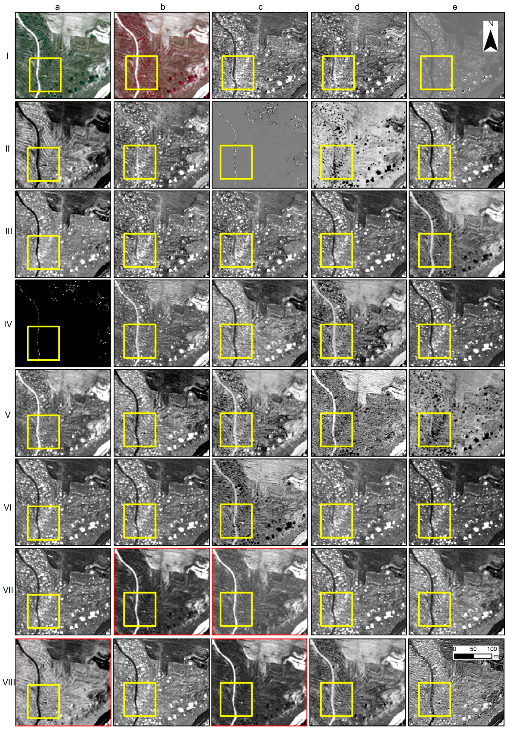
| No. | Index | Equation | Result in Figure 9 | Reference |
|---|---|---|---|---|
| 1 | Anthocyanin Reflectance Index 1 | c-I | [27] | |
| 2 | Anthocyanin Reflectance Index 2 | d-I | [27] | |
| 3 | Atmospherically Resistant Vegetation Index | e-I | [28] | |
| 4 | Burn Area Index | a-II | [29] | |
| 5 | Difference Vegetation Index | b-II | [30] | |
| 6 | Enhanced Vegetation Index | c-II | [31] | |
| 7 | Global Environmental Monitoring Index | d-II | [32] | |
| 8 | Green Atmospherically-Resistant Index | e-II | [33] | |
| 9 | Green Difference Vegetation Index | a-III | [34] | |
| 10 | Green Normalized Difference Vegetation Index | b-III | [35] | |
| 11 | Green Ratio Vegetation Index | c-III | [34] | |
| 12 | Infrared Percentage Vegetation Index | d-III | [36] | |
| 13 | Iron Oxide | e-III | [37] | |
| 14 | Leaf Area Index | a-IV | [38] | |
| 15 | Modified Chlorophyll Absorption Ratio Index | b-IV | [39] | |
| 16 | Modified Chlorophyll Absorption Ratio Index-Improved | c-IV | [40] | |
| 17 | Modified Non-Linear Index | d-IV | [41] | |
| 18 | Modified Simple Ratio | e-IV | [42] | |
| 19 | Modified Triangular Vegetation Index | a-V | [38] | |
| 20 | Modified Triangular Vegetation Index-Improved | b-V | [40] | |
| 21 | Non-Linear Index | c-V | [43] | |
| 22 | Normalized Difference Mud Index | d-V | [44] | |
| 23 | Normalized Difference Snow Index | e-V | [45] | |
| 24 | Normalized Difference Vegetation Index | a-VI | [46] | |
| 25 | Optimized Soil Adjusted Vegetation Index | b-VI | [47] | |
| 26 | Red Edge Position Index | Maximum derivative of reflectance in the vegetation red edge region of the spectrum in microns from 690 nm to 740 nm | c-VI | [48] |
| 27 | Renormalized Difference Vegetation Index | d-VI | [49] | |
| 28 | Simple Ratio | e-VI | [50] | |
| 29 | Soil Adjusted Vegetation Index | a-VII | [51] | |
| 30 | Sum Green Index | Mean of reflectance across the 500 nm to 600 nm portion of the spectrum | b-VII | [52] |
| 31 | Transformed Chlorophyll Absorption Reflectance Index | c-VII | [53] | |
| 32 | Transformed Difference Vegetation Index | d-VII | [54] | |
| 33 | Visible Atmospherically Resistant Index | e-VII | [55] | |
| 34 | WorldView Built-Up Index | a-VIII | [56] | |
| 35 | WorldView Improved Vegetative Index | b-VIII | [56] | |
| 36 | WorldView New Iron Index | c-VIII | [56] | |
| 37 | WorldView Non-Homogeneous Feature Difference | d-VIII | [56] | |
| 38 | WorldView Soil Index | e-VIII | [56] |
© 2017 by the authors. Licensee MDPI, Basel, Switzerland. This article is an open access article distributed under the terms and conditions of the Creative Commons Attribution (CC BY) license (http://creativecommons.org/licenses/by/4.0/).
Share and Cite
Agapiou, A.; Lysandrou, V.; Hadjimitsis, D.G. Optical Remote Sensing Potentials for Looting Detection. Geosciences 2017, 7, 98. https://doi.org/10.3390/geosciences7040098
Agapiou A, Lysandrou V, Hadjimitsis DG. Optical Remote Sensing Potentials for Looting Detection. Geosciences. 2017; 7(4):98. https://doi.org/10.3390/geosciences7040098
Chicago/Turabian StyleAgapiou, Athos, Vasiliki Lysandrou, and Diofantos G. Hadjimitsis. 2017. "Optical Remote Sensing Potentials for Looting Detection" Geosciences 7, no. 4: 98. https://doi.org/10.3390/geosciences7040098
APA StyleAgapiou, A., Lysandrou, V., & Hadjimitsis, D. G. (2017). Optical Remote Sensing Potentials for Looting Detection. Geosciences, 7(4), 98. https://doi.org/10.3390/geosciences7040098