Article

Exploitation of Satellite A-DInSAR Time Series for Detection, Characterization and Modelling of Land Subsidence

1
Department of Earth and Environmental Sciences, University of Pavia, Via Ferrata 1, 27100 Pavia, Italy
2
British Geological Survey, Natural Environment Research Council, Nicker Hill, Keyworth, Nottinghamshire NG12 5GG, UK
3
Geohazards InSAR Laboratory and Modeling Group, Instituto Geológico y Minero de España (IGME), C/. Alenza 1, 28003 Madrid, Spain
4
Unidad Asociada de Investigación IGME-UA de Movimientos del Terreno Mediante Interferometría Radar (UNIRAD), Universidad de Alicante, P.O. Box 99, 03080 Alicante, Spain
5
Earth Observation and Geohazards Expert Group (EOEG), EuroGeoSurveys, the Geological Surveys of Europe, 36–38, Rue Joseph II, 1000 Brussels, Belgium
6
CGG, NPA Satellite Mapping, Crockham Park, Edenbridge Kent TN8 6SR, UK
7
Departamento de Ingeniería Civil, Escuela Politécnica Superior, Universidad de Alicante. P.O. Box 99, 03080 Alicante, Spain
*
Author to whom correspondence should be addressed.
Geosciences 2017, 7(2), 25; https://doi.org/10.3390/geosciences7020025
Submission received: 28 February 2017 / Revised: 4 April 2017 / Accepted: 6 April 2017 / Published: 11 April 2017
(This article belongs to the Special Issue Observing Geohazards from Space)

Abstract

:
In the last two decades, advanced differential interferometric synthetic aperture radar (A-DInSAR) techniques have experienced significant developments, which are mainly related to (i) the progress of satellite SAR data acquired by new missions, such as COSMO-SkyMed and ESA’s Sentinel-1 constellations; and (ii) the development of novel processing algorithms. The improvements in A-DInSAR ground deformation time series need appropriate methodologies to analyse extremely large datasets which consist of huge amounts of measuring points and associated deformation histories with high temporal resolution. This work demonstrates A-DInSAR time series exploitation as valuable tool to support different problems in engineering geology such as detection, characterization and modelling of land subsidence mechanisms. The capabilities and suitability of A-DInSAR time series from an end-user point of view are presented and discussed through the analysis carried out for three test sites in Europe: the Oltrepo Pavese (Po Plain in Italy), the Alto Guadalentín (Spain) and the London Basin (United Kingdom). Principal component analysis has been performed for the datasets available for the three case histories, in order to extract the great potential contained in the A-DInSAR time series.

1. Introduction

Land subsidence represents the main response to superficial and deep deformations induced by multiple natural and anthropic phenomena (i.e., vadose zone processes, such as swelling/shrinkage of clay soils, soil consolidation, aquifer compaction, solid and fluid extraction, and load-induced compaction) which take place at different spatio-temporal scales. The impacts of land subsidence can be infrastructural, economic, environmental, and social [1,2], including impacts on the natural heritage, natural surficial drainage system, agricultural activities, building foundations and transportation network, alteration of irrigation network, reduction of aquifer storage, ground failure, and it enhances the risk of floods, affecting the human life and activities. The increasing factors of risk are mainly due to rapid urban development, relatively young alluvium soils, and weak mitigation and adaptation strategies [3]. Therefore, in the pre-mitigation investigation phase, the identification of land subsidence areas and the understanding of driving factors is fundamental in order to adopt suitable land use planning and sustainable management of the available resources. Then, land subsidence investigations are essential to delineate the magnitude and type of deformation related to the temporal evolution of surface displacements (i.e., linear or non-linear), the spatial extension of the affected areas and the mechanism of land subsidence.
When land subsidence evidence is the result of superimposed processes, it is difficult to discern, and to map the different processes and to evaluate the associated triggering factors. Therefore, the complexity of the mechanism recognition requires a multidisciplinary approach including the expertise of engineering geologists, hydrogeologists, and geotechnical engineers. Until now, the scientific community carried out different strategies and a combination of different methods, including field measurements, remote sensing tools, and integrated approaches, to solve the complexity of the problem in many areas of the world [4,5,6,7,8].
Recent advanced ground deformation investigations make use of satellite synthetic aperture radar (SAR) data to examine the mechanisms of land subsidence around the world. In particular, these investigations exploit advanced differential interferometric synthetic aperture radar (A-DInSAR) techniques, which are based on the processing of multiple interferograms derived from a large set (at least 20 images) of SAR images. These techniques allow the retrieval of displacement time series of measuring points over wide areas at millimeter resolution [9,10,11,12,13,14,15] and have already been successfully applied to monitoring the evolution of different processes.
In the last two decades, A-DInSAR techniques have experienced major developments, which are mainly related to (i) the progress of satellite SAR data acquired by new missions, such as COSMO-SkyMed and ESA’s Sentinel-1 constellations; and (ii) the development of novel processing algorithms. The improvements in the displacement time series (TS) obtained by A-DInSAR techniques need appropriate methodologies to analyze extremely large datasets which consist of very large amounts of measuring points and associated deformation histories with high temporal resolution.
This work contributes to address this crucial aspect, by exploiting the great potential contained in A-DInSAR time series. In this article, the relevant contributions of A-DInSAR time series are analyzed distinguishing the main advantages and limitations for three topics that commonly concern land subsidence investigations:
  • Detection of the magnitude and distribution of land subsidence;
  • Characterization of the mechanisms involved in land subsidence; and
  • Modelling of land subsidence due to groundwater level changes.
In particular, the paper provides insights into A-DInSAR time series capabilities and suitability as valuable supporting tools for these topics through interesting case histories of moderate rates of displacement in flat areas (Oltrepo Pavese, Po Plain, in Italy) and of land subsidence due to groundwater level change (Alto Guadalentín Basin, in Spain and the London Basin, in the United Kingdom). A-DInSAR time series analysis has emerged as a fundamental tool not only to monitor, but also to detect, ground motion areas. An innovative approach based on A-DInSAR time series analysis is presented to detect ground motion areas with significant deformational behaviors, such as linear, non-linear, and seasonal movements. Moreover, displacement time series acquired by multi-temporal SAR sensors allow the extraction of a historical archive of the temporal evolution of land movements. The collection of multi-sensor displacement time series proved to be crucial for the characterization of land subsidence mechanisms, such as transient and inelastic aquifer deformation otherwise undetectable by considering the average velocity. Finally, changes, such as acceleration and deceleration in the displacement rates, were simulated by calibrating a 1-D model using A-DInSAR time series.

2. Data and Methods

In the framework of the Panel on Land Subsidence of the U.S. National Research Council (NRC) (1991) two information needs were recognized [16]:
  • Earth-science data and information on the magnitude and distribution of land subsidence in order to recognize and to assess future problems; and
  • Research on subsidence processes and engineering methods in order to prevent damage.
According to these information needs, the support of A-DInSAR time series for land subsidence investigations is presented here. A multidisciplinary approach was adopted by combining geological, geotechnical, hydrogeological, and A-DInSAR data to gain insight into land subsidence detection, characterization, and modelling through three representative test cases: Oltrepo Pavese, in Italy, Alto Guadalentín Basin, in Spain, and the London Basin, in the United Kingdom (Figure 1).
Regarding the detection of ground motion areas, a novel methodology was implemented in the plain area of the Oltrepo Pavese (Italy) in order to distinguish different components of motion. The characterization of the mechanisms of land subsidence were analyzed in detail in the Alto Guadalentín Basin in Spain, where the highest subsidence rates measured in Europe (>10 cm/year) were recognized as a direct consequence of long-term aquifer exploitation [17]. Finally, the London Basin was chosen as a study area to use the A-DInSAR time series to characterize the hydrological properties of the deposits of the basin and to integrate the A-DInSAR time series in the modelling of ground deformation. The prediction of the ground motion expected in response to the groundwater level variations was performed in the London Basin thanks to the availability of detailed time-series data from the observation borehole network provided by the Environment Agency (around ~200 piezometers), to reconstruct the historical groundwater level changes across the basin for the 1990s and 2000s.
Additional details about the data for each test case are summarized in Table 1.

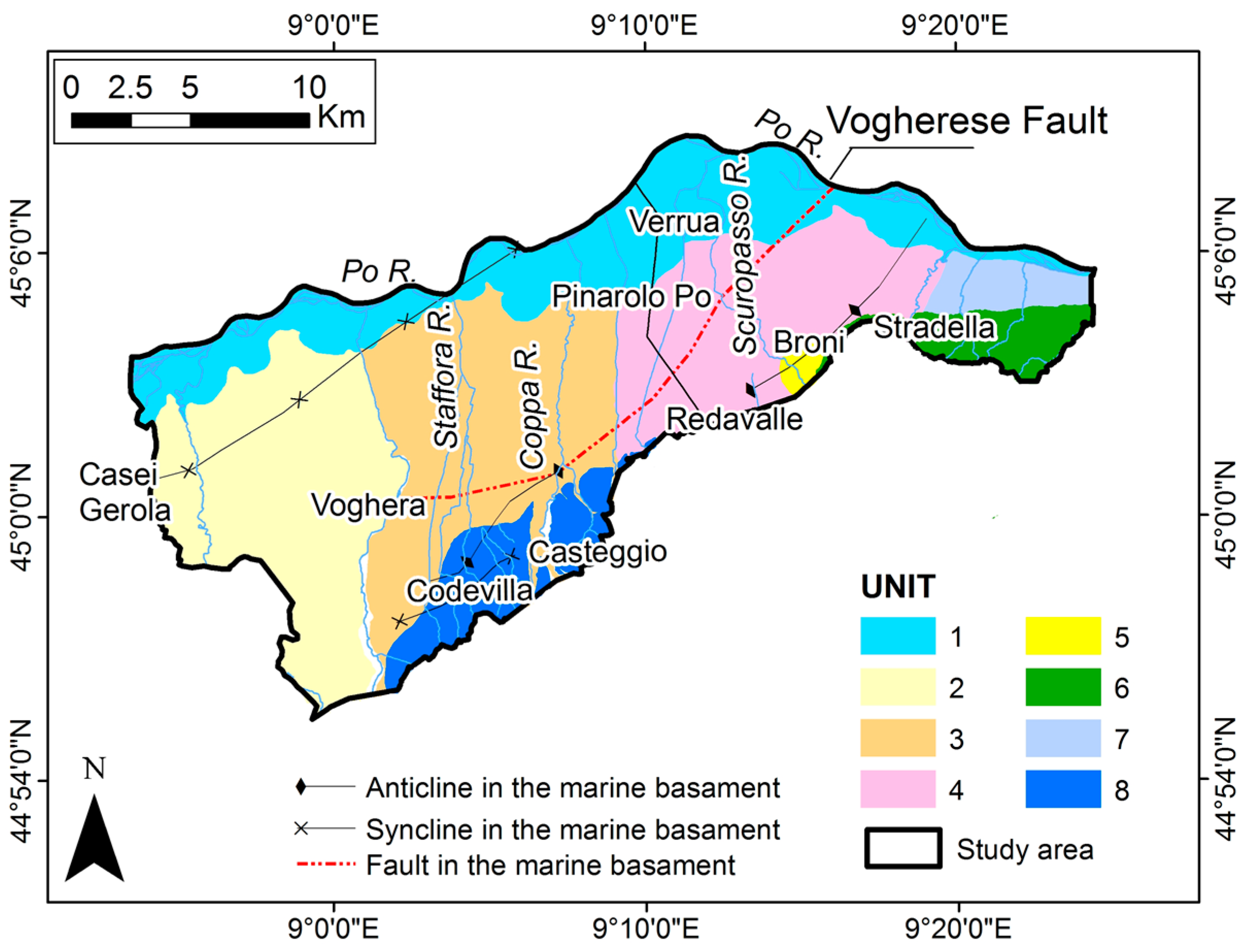
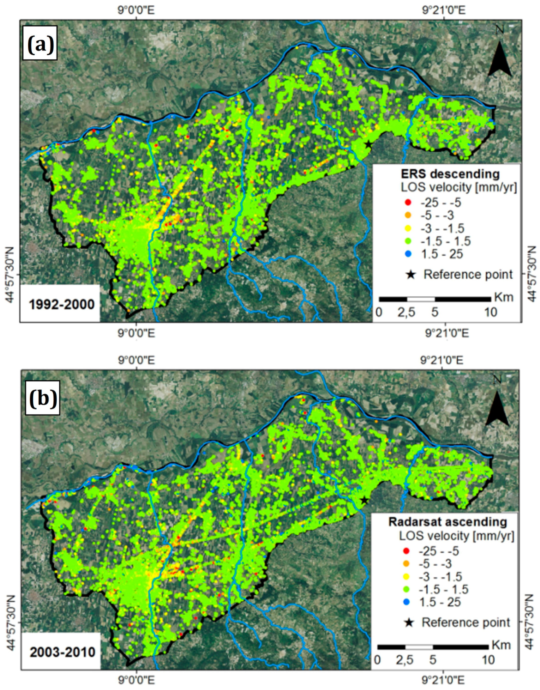
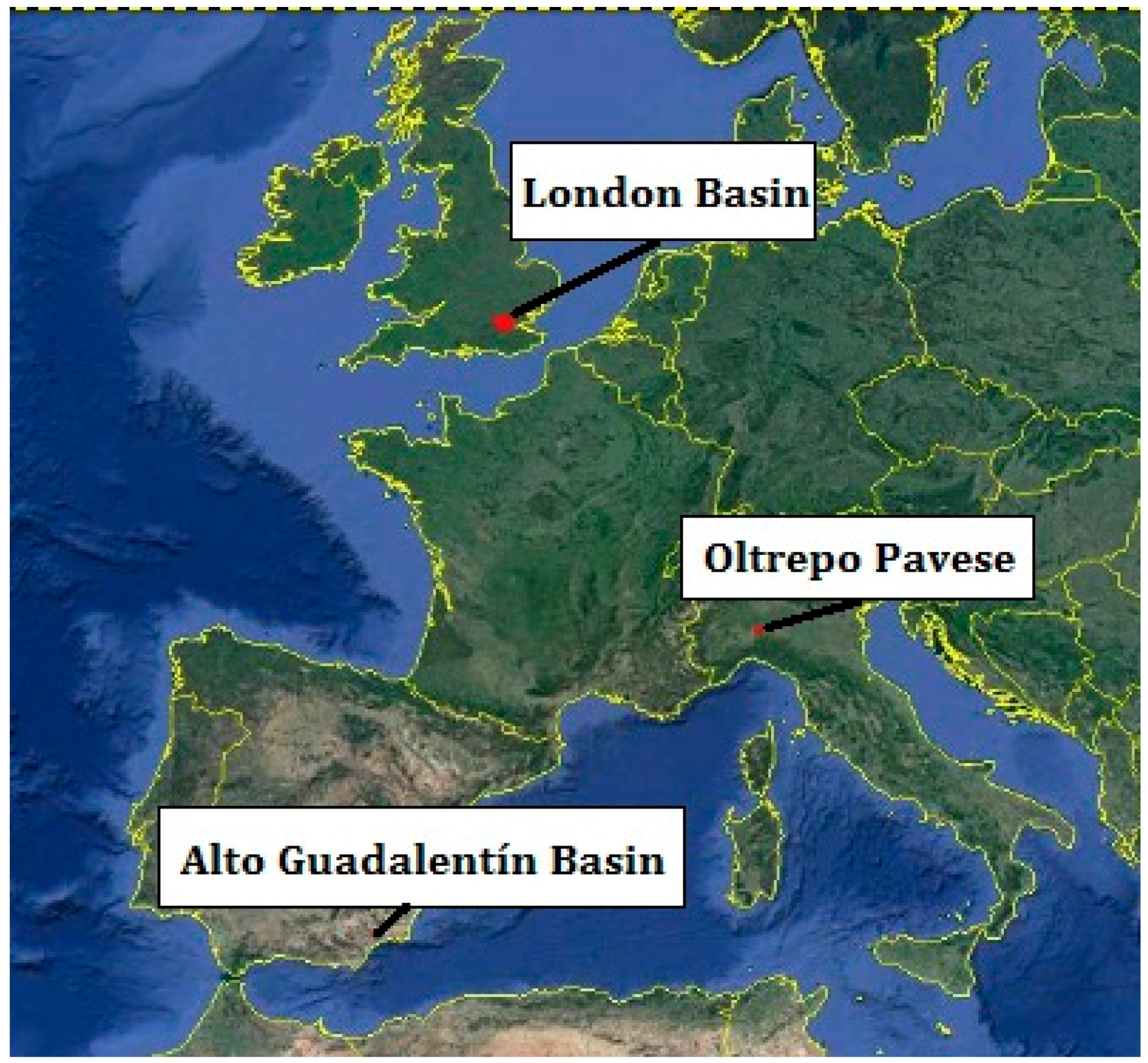
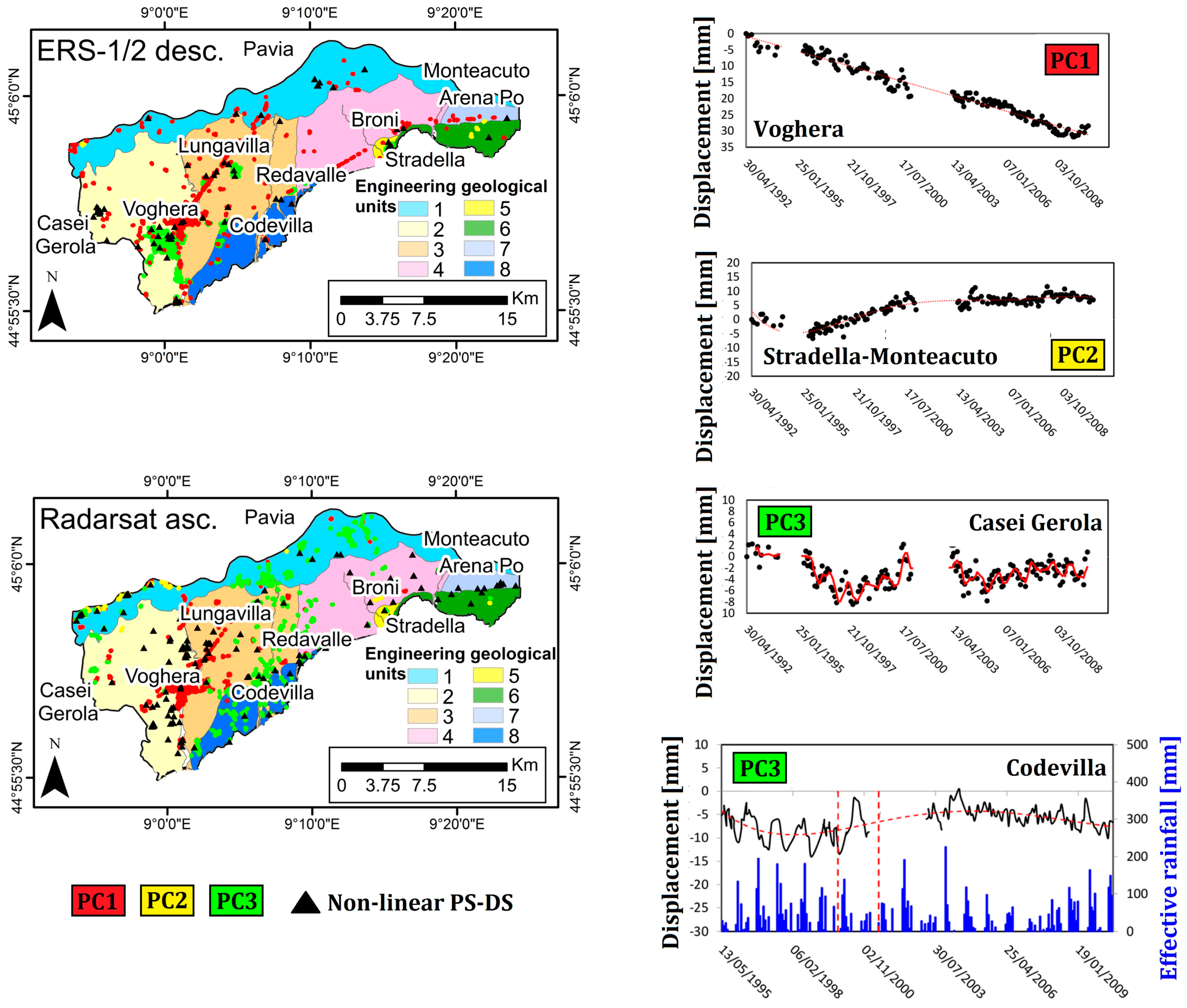
2.1. The Oltrepo Pavese Test Case

The Oltrepo Pavese (Italy) is the plain sector of the Po River (Figure 2) covering an area of approximately 440 km2. The Oltrepo Pavese is a representative site of similar geological contexts in the Po Plain, where geohazards, due to natural and anthropic factors, were previously recognized [18]. Severely damaged structures were also observed in this area due to volume changes of clayey soils (shrinkage and swelling during drying and wet periods, respectively). Regarding the land use coverage of Oltrepo Pavese, discontinuous urban fabrics are the most prevalent land use class and 68% of the monitored area is covered by non-irrigated arable land.
The plain of the Oltrepo Pavese is constituted by alluvial quaternary deposits, originated from the action of Apennine streams and of the Po River [19,20]. These deposits overlay Miocene-Pliocene marine substratum, composed of sandy-marls, sandstones, conglomerates, gypsy-marls, and calcareous-marls. Three main geomorphological units were previously distinguished [20,21] in the quaternary deposits (1) Post-würmian alluvial deposits; (2) Würmian-holocenic alluvial deposits; (3) Pre-würmian alluvial deposits.
Post-würmian alluvial deposits are the most recent sediments that are mainly localized close to the Po River. These deposits are composed of sand, sandy silt, and silt, and they contain a shallow phreatic aquifer.
Würmian-holocenic alluvial deposits are made up of alternating sand and gravel, with interbedded clays or argillaceous silt. These deposits contain a shallow phreatic aquifer and deeper aquifers, of both phreatic and confined types. The aquifer geometry is controlled by the deeply buried structures in the tertiary marine basement, consisting of a series of folds and fold-faults. These alluvial deposits are extensively covered by clayey-silty deposits, which act as a seal, limiting water infiltration [22].
Pre-würmian alluvial deposits, located in the southern part of the study area, consist of older fluvial terraces, and are composed of gravel and sand with a silty matrix. In the Pre-würmian unit, the depth of the groundwater level in this unit reaches values up to 20 m depth.
Regarding the Quaternary sediment thickness, a decrease from west to east is observed in the study area. The minimum thickness and the outcrop of the marine substratum is evident in correspondence with the Stradella thrust, where neotectonic activity was previously described [23].
The geotechnical properties of the Quaternary deposits in the first 15 m of depth of the Oltrepo Pavese plain are summarized in Figure 2 [24]. Six geotechnical classes of non-cohesive soils (from I1 to I6) and four geotechnical classes of cohesive soils (from C1 to C4) have been distinguished. Therefore, taking into account the geotechnical classification of these soils, eight engineering geological units were introduced as representative of homogeneous geotechnical profiles (Figure 2). Unit 1 represents the Post-würmian alluvial deposit of the Po River, and is mainly constituted of non-cohesive soils (I3). Conversely, units 2, 3, 4, and 7 are Würmian-holocenic alluvial deposits, characterized by cohesive soils. Unit 5 is composed of the alluvial fan of the Scuropasso River, and units 6 and 8 by the Pre-würmian terraced deposits.
The A-DInSAR dataset available for the Oltrepo Pavese test case is composed of SAR images acquired by sensors operating in the C-band (wavelength: 5.6 cm; frequency: 5.3 GHz) onboard the ERS-1, ERS-2, and RADARSAT-1 (RSAT) satellites. The scenes were acquired in the ascending mode, covering the time intervals from 9 July 1992 to 2 August 2000, and from 24 March 2003 to 5 May 2010. The dataset acquired in the descending mode covers the time intervals from 3 April 1992 to 7 January 2001 and from 28 April 2003 to 5 January 2009. The ERS-1/2 images were acquired with a nominal repeat cycle of 35 days, while the RADARSAT images were acquired with a revisiting period of 24 days. These scenes were processed with the SqueeSAR™ technique by Tele-Rilevamento Europa (TRE srl, Milano, Italy). The algorithm allows the extraction of movement measurements, not only from traditional persistent scatterers (PS), such as anthropic structures or rocks, but also from distributed scatterers (DS), such as sparse vegetated areas [10]. This permitted to have a high density of A-DInSAR data over non-urban areas. ERS-1/2 descending and RADARSAT-1 ascending data were exploited to monitor the time intervals, from 1992 to 2000, and from 2003 to 2010 (Figure 3), in order to analyze the datasets with higher spatial and temporal resolutions.
Various geohazard-mapping methodologies were previously implemented by the use of A-DInSAR techniques [25,26,27,28,29,30]. The problem of detection of land subsidence using A-DInSAR data is compounded by the large-scale analysis of an enormous amount of measuring points. Often, the strategies to detect and to map the land subsidence areas are based on the spatial distribution of the average velocities and on statistic approaches to automatically detect clusters with significant movements. Some difficulties were observed to distinguish ground deformation due to different processes, or in detecting shallow deformations caused by seasonal processes.
In this work, the procedure proposed by [31] is exploited for the identification of land subsidence areas and to disentangle the contribution of different processes to the spatial and temporal distribution of displacement estimated through multisensor A-DInSAR time series. The first step of the performed activity was the decomposition of the vertical and E-W components of motion and the displacement time series (TS) accuracy assessment. Then, different statistical tests, such as the principal component analysis (PCA) and an automated time series classification, were applied. Thereafter, areas with significant movement, so-called “ground motion areas”, were mapped. These areas correspond to a cluster of a minimum 3 of PS, with a maximum distance of 50 m, characterized by the same trends (i.e., linear, non-linear, and seasonal). Furthermore, the methodology to detect ground motion areas using the average velocity [25] was implemented in the same area using ERS-1/2 and Radarsat data to assess the results.

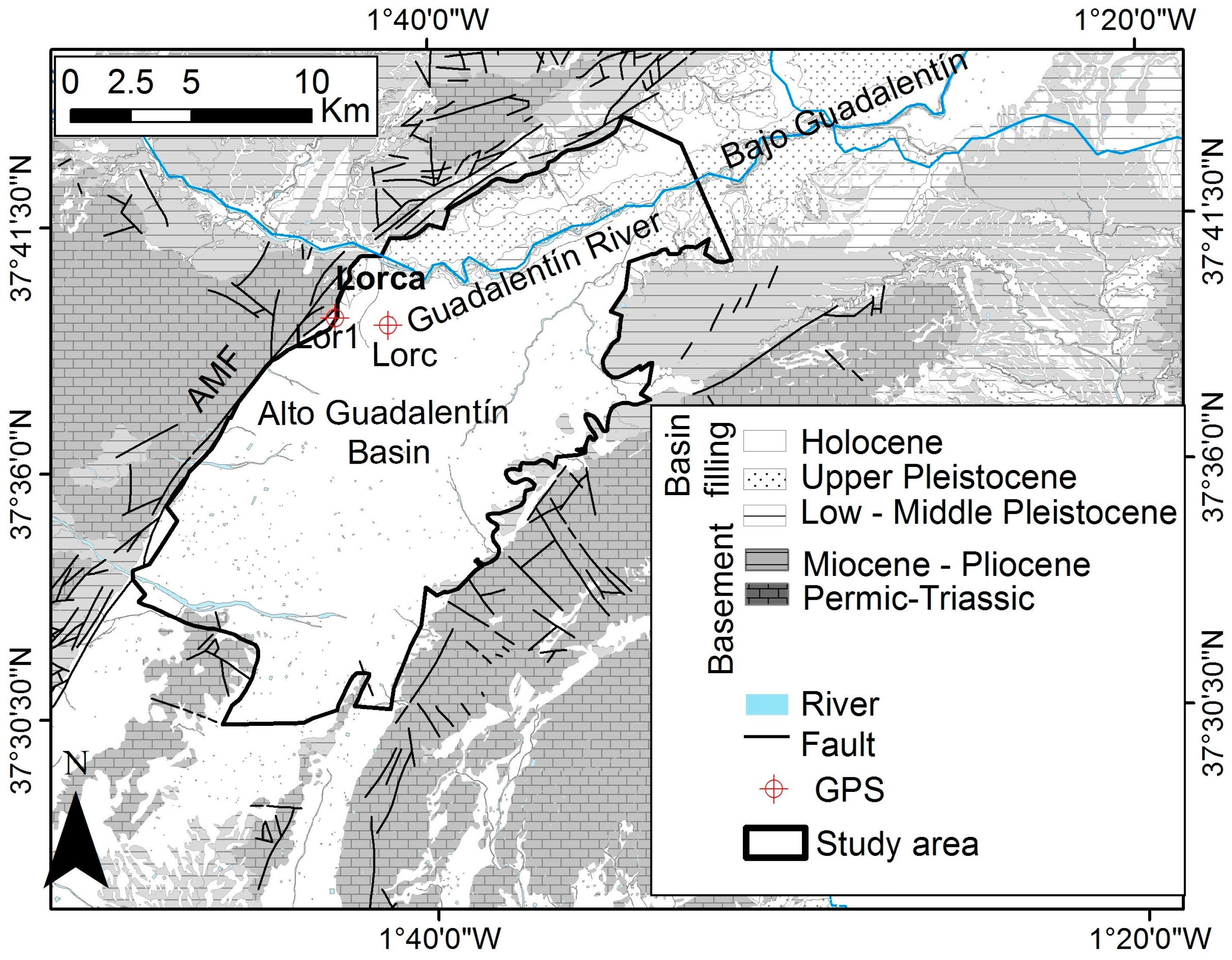
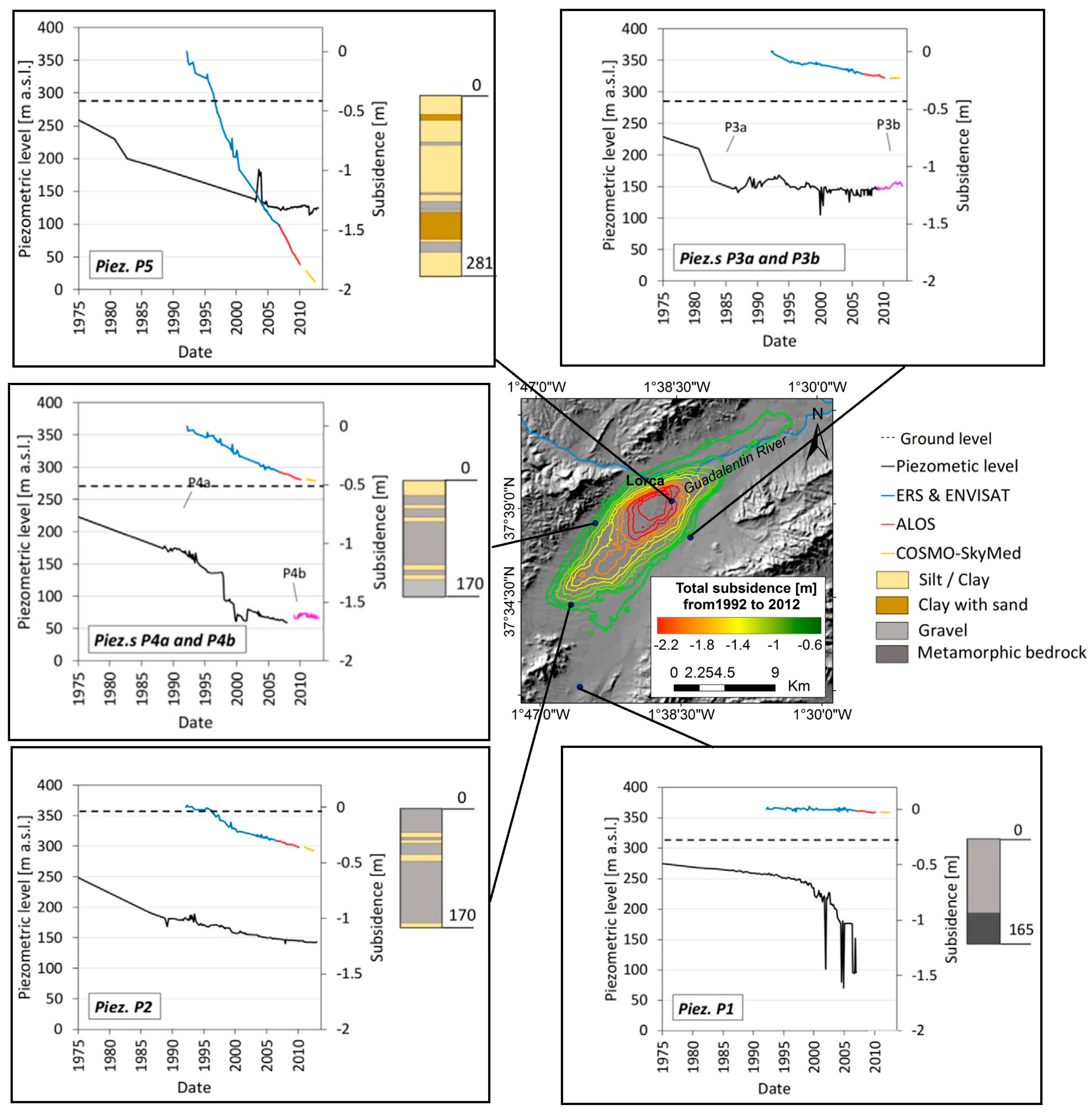
2.2. The Alto Guadalentín Test Case

The Guadalentín Basin is located in Southeast Spain, and has an extension of 277 km2 (Figure 4). The area was chosen because the highest subsidence rates measured in Europe (>10 cm/year) have been recorded here, as a direct consequence of long-term aquifer exploitation. Urban sites are located in the area, but agriculture is the prevalent land use.
The Guadalentín Basin is underlain by Neogene-Quaternary sediments transported by the Guadalentín River along an intramontane depression located in the eastern part of the Baetic Cordillera, which is an ENE-WSW-oriented alpine orogenic belt resulting from the ongoing convergence of the African and Iberian plates [32]. The Guadalentín is a tributary river of the Segura River which geographically divides the Bajo from the Alto Guadalentín sub-basins, where Lorca City is located (Figure 4). The basin is mainly composed of Quaternary alluvial fan systems that overlap with Tertiary deposits. The Tertiary deposits are composed of conglomerate and calcarenite that outcrop at the border of the basin. The main active fault system of the study area, the NE-SW-oriented Alhama de Murcia Fault (AMF) [33] is represented in Figure 4. The deposits of the basin overlap the Paleozoic metamorphic complexes [34].
The Alto Guadalentín aquifer system is characterized by Plio-Quaternary detrital and alluvial material, including clays, sands, and conglomerates with clay and/or silt matrices; Miocene detritical with conglomerate and sand deposits; and local Triassic carbonate rocks (Figure 4). The lower impermeable limit of the aquifer is composed of Mesozoic marl, and marl with intercalated sand and conglomerates. The aquifer geometry is controlled by the horst and graben structures of the impermeable limit [35]. Since 1960, agricultural advance has led to the exploitation of the aquifer system, which resulted in the aquifer being declared temporarily overexploited in 1987 [36]. Historically, the piezometric level was close to the surface and, as artesian wells were exploited, groundwater drawdown became apparent in 1972 [35].
The A-DInSAR datasets available for the Alto Guadalentín are C-band (ERS-1, ERS-2, and ENVISAT), L-band (ALOS PALSAR), and X-band SAR data (COSMO-SkyMed). ERS-1/2 and ENVISAT scenes were acquired in the descending mode, covering the time intervals from 22 June 1992, to 21 December 2000, and from 15 March 2003 to 15 March 2007. ALOS PALSAR and COSMO-SkyMed scenes were acquired in the ascending mode, covering the time intervals from 19 January 2007 to 14 June 2010, and from 17 May 2011 to 14 October 2012. The SAR images acquired by ERS-1, ERS-2, and ENVISAT sensors were processed using the small baseline approach [13,38]. For each dataset, we first used Delft Object-oriented Radar Interferometric Software (DORIS) [11] to produce the interferograms and then we performed the time series analysis using Stanford Method for Persistent Scatterers (StaMPS) [15]. Finally, results from both datasets were merged to determine the temporal evolution of displacement over the complete ERS-ENVISAT period. ALOS PALSAR and COSMO-SkyMed dataset were processed using SPN software [12,14]. The use of the A-DInSAR dataset acquired by different sensors using different incidence angles clearly affects the capability to measure the vertical component of the displacement. More precisely, ERS-1/2 and ENVISAT have a 23° incidence angle, which allows the estimation of 92% of vertical displacements, while ALOS and COSMO-SkyMed satellites only detect 83% and 75% of vertical displacements, respectively. As a result, the identification of these geometrical distortions due to the different acquisition angles of the various sensors is essential to perform A-DInSAR analyses. Consequently, LOS velocities have been projected along the vertical direction for each dataset in order to homogenize the datasets (Figure 5). Furthermore, local comparisons were performed with Global Positioning System (GPS) data available for two continuous stations (see the location in Figure 4) located in the study area, demonstrating the high consistency of the vertical motion measurements between the two different surveying techniques. An average absolute error of 4.6 ± 4 mm for the ALOS data and of 4.8 ± 3.5 mm for the COSMO-SkyMed data confirmed the reliability of the projection along the vertical direction [39].
The land subsidence triggered by groundwater exploitation depends on three main factors [4]: the areal and vertical distribution of subsidence-prone materials, their current state of stress, and their stress history. Previous works highlight that the same aquifer system can exhibit different deformation responses, according to the stratigraphic characteristic and the amount of groundwater pumped. Indeed, the complexity of the deformation responses to the applied stress is due to the different composition of the hydrostratigraphic units and the different changing patterns of groundwater levels that the units have experienced [40]. Principal component analysis was performed using the ERS and ENVISAT, ALOS, and COSMO-SkyMed data to analyze the spatio-temporal deformation pattern of each dataset. Then, A-DInSAR and piezometers time series have been compared to give insights about the evolution of the aquifer deformation behavior across the basin.

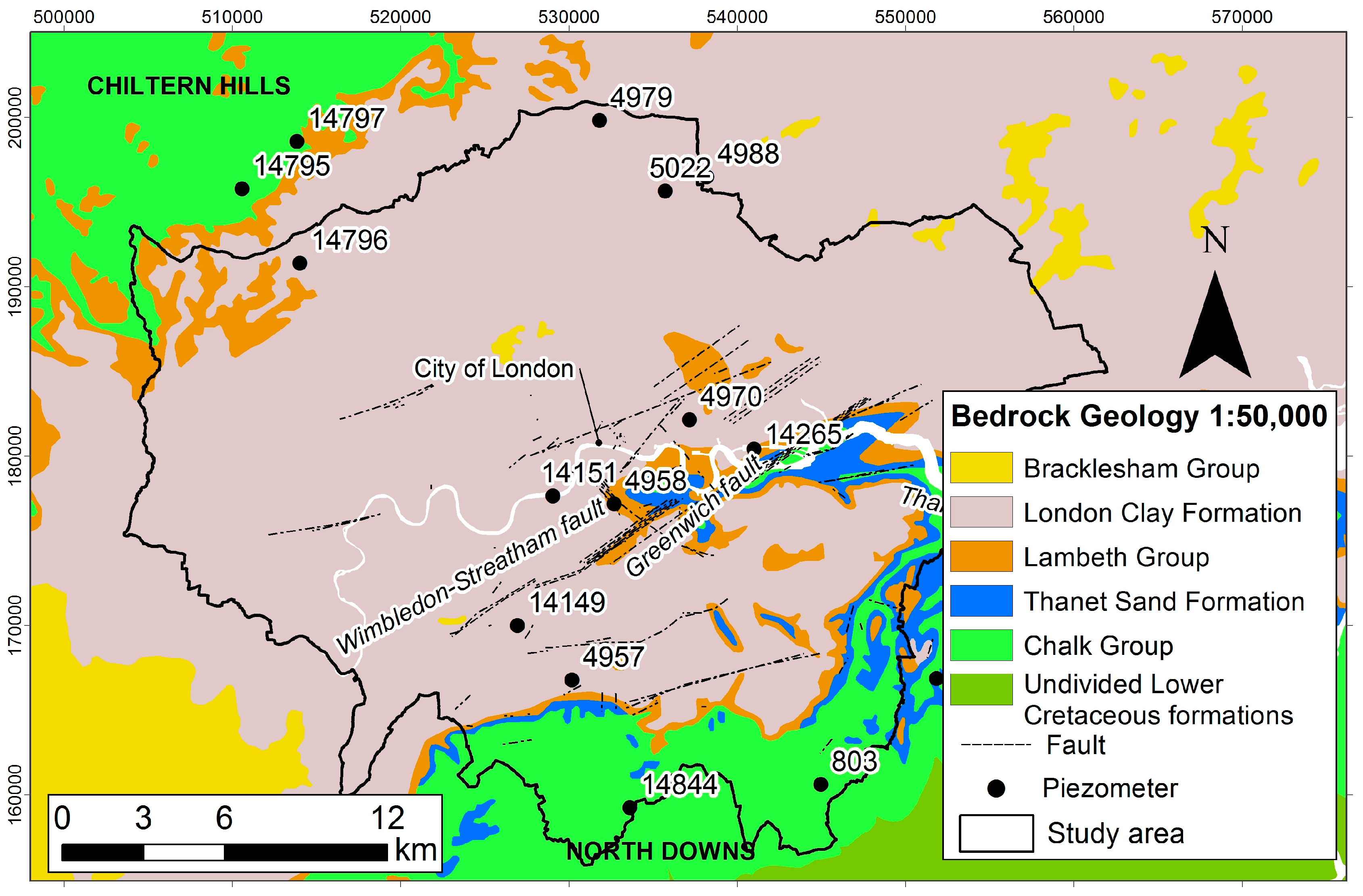
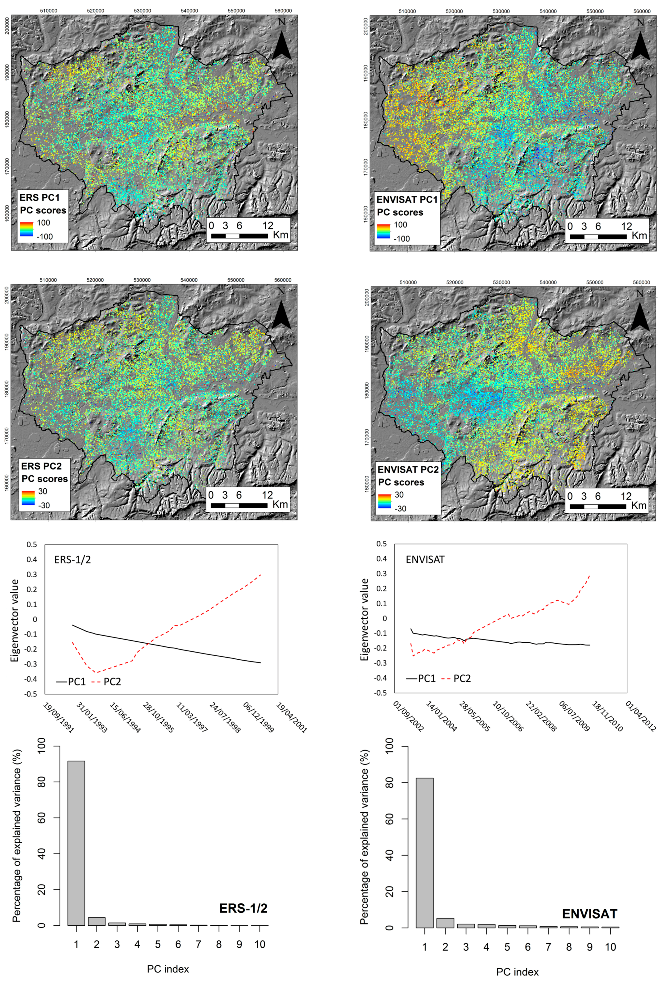
2.3. The London Basin Test Case

The study area located in the London Basin (Southern England) covers an extension of about 1360 km2 (Figure 6). This test site was chosen to model land subsidence due to groundwater level change by applying a 1D model, thanks to the large availability of geological, hydrogeological, and geotechnical data. The London Basin is a densely-urbanized area, where, London, the capital and largest city in the United Kingdom, and the most populated in Europe, is located. The basin overlies the Palaeozoic basement, which is bounded to the south by the Variscan Front [41]. The basin is underlain by Paleogene deposits that overlie the Chalk Group [42,43]. These deposits comprise the Thanet Formation, mainly composed of a fine sand; the Lambeth Group, consisting of vertically- and laterally-variable sequences, mainly of clay with silty and sandy horizons; the Harwich Formation, a silty, sandy clay with gravel beds, and; the London Clay Formation, a dense, fissured clay [44,45]. Quaternary deposits, primarily river terrace deposits, are associated with the River Thames and artificially modified ground. The city of London lies within a graben bounded by the Northern Boundary fault to the north and the Wimbledon-Streatham fault and the Greenwich fault to the south.
The Chalk Group is the principal aquifer in the London Basin supporting both public water and industrial groundwater use supply [46,47]. In the central area of the basin, the chalk aquifer is confined by the overlying Palaeogene formations. The chalk aquifer is recharged on the interfluves—in the Chiltern Hills to the north and North Downs to the south, where the Chalk outcrops and the aquifer becomes unconfined. The unconfined aquifer is characterized by larger seasonal water table variations, where fracture lineaments represent the main river drainage systems [48]. The lithological variations and the faulting on the chalk aquifer have a key control on the variability of the aquifer properties across the Thames Basin [49]. Historic overexploitation of the Chalk aquifer up to the 1960s led to widespread lowering of groundwater levels, reaching a depth of up to 90 m below sea-level in the central London Basin [46]. Thus, the Chalk aquifer became unconfined, leading to under-drainage and desaturation of the London Clay [41,46]. In the mid-1960s, Chalk groundwater level rapidly recovered at a rate of up to 3 m/year [46]. Therefore, an action plan was developed by the London Underground, Thames Water and the Environment Agency (EA) (i.e., the GARDIT, General Aquifer Research Development and Investigation Team) strategy to control groundwater recovery and re-saturation of the London Clay, that could potentially have negative impacts on the foundations of structures and infrastructure in the basin. Thus, the EA implemented an observation borehole network within the basin in order to monitor and manage changes in groundwater levels. Furthermore, an artificial recharge scheme was licensed in North London, NLARS (North London Artificial Recharge Scheme; [46]) to support the groundwater levels control [49,50].
The A-DInSAR datasets available for the London Basin are ERS-1 and ERS-2 SAR scenes acquired in ascending and ENVISAT scenes acquired in descending mode. The first dataset covers the time interval from 19 June 1992 to 31 July 2000 and the second one from 13 December 2002 to 17 September 2010. The available scenes were processed using the GAMMA SAR and Interferometry software (Gamma Remote Sensing, Bern, Switzerland) and, in particular, the Interferometric Point Target Analysis (IPTA) algorithm [52]. Considering the horizontal movements negligible in the study area, LOS displacements and velocities were projected for both datasets along the vertical direction (Figure 7). Ninety-five percent of the PS targets within the study area show an uncertainty of the average LOS velocity in the range between 0.09 and 1.09 mm/year in the ERS-1/2 dataset, and between 0.17 and 1.13 mm/year in the ENVISAT dataset [53].
Principal component analysis was also performed across the London Basin, using ERS-1/2 and ENVISAT data, to identify spatio-temporal deformation patterns.
Furthermore, A-DInSAR time series were also exploited to simulate the ground motion response due to the changes in the groundwater level. Many authors have exploited A-DInSAR data for the calibration and validation of models in which the land subsidence is due to groundwater level variations [54,55,56,57]. In this study, A-DInSAR time series were integrated in a one-dimensional model (1-D) to simulate the ground motion in response to changes in hydraulic head in the Chalk aquifer. The 1-D model is based on the inversion of the equation introduced by [58] to calculate the storage coefficient (S):
S = ∆d/∆h
where ∆d is the vertical displacement as estimated by A-DInSAR time series ∆h. The assumption of one-dimensional consolidation is motivated by the hypothesis that the ground deformation is only vertical for this area, justified by the fact that the horizontal displacements are believed to not be significant [51]. The 1-D model assumes that the aquifer pore pressure instantaneously equilibrates with piezometric level changes in the aquifer and any time-lag between the piezometer level variations and the compaction of the geological layers is not accounted for. This assumption is justified by the inspection of the ground motion and groundwater records across the basin [51]. The simulation of the ground motion was conducted by using the following equation [59,60]:
∆d = S × ∆h
The simulation was performed at nine piezometers representative of semi-confined and confined aquifer condition using the average displacement time series within the buffer areas with a radius of 500 m from each piezometer. In the first step, the geological sequence was compared with the groundwater level variation to classify the aquifer state according to its confined condition (i.e., confined, semi-confined, unconfined) and the geological interval over which the piezometric head varied. Then, the aquifer storage coefficient (S) was calculated by using Equation (1) in the time interval where a good fit between piezometer data and average displacement time series was evident.
Finally, A-DInSAR time series were compared with the simulated ground motion in order to estimate the absolute average error of the model. Furthermore, the capability to use the A-DInSAR time series as the input of the model was assessed in order to simulate the hydraulic head changes. The inverted model was performed at piezometer 4988 (see the location in Figure 6) using the following equation:
∆h = ∆d/S

3. Results

3.1. Time Series Support for Detection of Land Subsidence: The Oltrepo Pavese Test Case

The outcomes of the A-DInSAR time series analysis acquired by ERS-1/2 and RADARSAT-1 sensors show that the Oltrepo Pavese is affected by three deformational behaviors with linear, non-linear, and seasonal trends. The cumulated displacements observed in the 1992–2000 period is higher than those detected in the period 2003–2010, and a decrease of deformation was observed.
The town of Voghera and the railway of Voghera–Pavia (Figure 8) are located in the most affected area by land subsidence with linear movements (principal component 1, PC1), with average LOS velocity in the range from −2 to −3.7 mm/year, in the period 1992–2000, and in the range of −2 to −4.8 mm/year in range of −2 to −4.8 mm/year, in the period 2003–2010. Areas of moderate uplift were observed via principal component 2 (PC2) of the ERS-1/2 and RADARSAT-1 data, in the sector from Stradella to Monteacuto (Figure 8), where geomorphic evidence of an active emergent thrust was previously observed [61]. Ground motion areas characterized by seasonal movements (principal component 3, PC3) are mainly located in the southern sector of Voghera and in proximity to Lungavilla, Codevilla, Casei Gerola, and Broni. The seasonal deformation behaviors in the Oltrepo Pavese are mainly due to seasonal fluctuations of the groundwater level and swelling-shrinkage of clayey soils [31]. Ground motion areas delineated using the PC3 of ERS-1/2 and RADARSAT-1 data in proximity of Codevilla (see location in Figure 8) match with an area where a high density of damaged buildings was recorded [62]. This site is located over Engineering Geological Unit 8, where shallow alluvial deposits of the first 8 m of depth exhibit swelling potentials from medium to very high [62]. The seasonal component of motion detected in the TS is directly correlated with the effective rainfall detected at the nearest pluviometric station, located in Voghera (Figure 8).
Changes in trends in the displacement time series were observed at the end of 1999 and 2008 in the areas of Broni, Voghera, Lungavilla, and Casei Gerola, and, in most of the cases, the non-linear trend are superimposed on seasonal ground motion areas identified using PC3.
Even though the average velocity may be useful to detect physical processes characterized by linear trends, the same parameter seems not to be efficient in detecting ground motion areas affected by non-linear and seasonal movements. The challenge of exploitation of the time series to detect the ground motion areas is to take into account different deformational behaviors. Hence, the reliability of the results clearly depends on the quality of the time series. Consequently, post-processing checks of the time series are fundamental to remove problems due to phase unwrapping, regional unreal trends, and anomalous displacement detected on certain dates [31]. Anomalous displacements were recorded on 9 March 1997 and 16 July 2000 by the ERS-1/2 descending datasets, and on 10 December 2008, for the RADARSAT-1 ascending dataset in the Oltrepo Pavese. The anomalous displacement identified in the RADARSAT-1 dataset might be related to the snowfall that occurred on the day of the SAR acquisition. Thus, these SAR scenes were not included in the following analyses.
Furthermore, the same A-DInSAR datasets were analyzed using the methodology based on the average velocity [25] in order to validate the areas detected using the PC1 and to assess the results obtained using these different approaches. The distribution of the so-called “anomalous areas” is represented in Figure 9. Eighty-four percent of the anomalous areas detected in the period from 1992 to 2000 and from 2003 to 2010 coincide with ground motion areas detected using the PC1 of the ERS-1/2 and Radarsat data, respectively. Three and seven percent, respectively, of the anomalous areas detected in the period from 1992 to 2000 and from 2003 to 2010 coincide with ground motion areas detected via PC2. Three percent of the anomalous areas corresponds to ground motion areas detected via PC3 using ERS-1/2 and Rasarsat data. Therefore, 10% and 6% of the anomalous areas are not detected using PCA-based methodology. However, the extension of these areas reaches values of 0.2–0.3 km2, resulting in localized movements. Otherwise, the approach based on the average velocity allows the detection of 35% and 69% of the ground motion areas detected via PC1 of the ERS-1/2 and Radarsat data. Seventy-two and sixty-seven percent, respectively, of the ground motion areas detected via PC2 can be identified using the average velocity of ERS and Radarsat data. Finally, 51% and 11% of the ground motion areas detected via PC3 of the ERS and Radarsat data, respectively, can be mapped using the average velocity. Overall, the results demonstrate that, when using the PCA-based methodology, most of anomalous areas based on the average velocity can be detected and, as expected, ground motion areas mainly due to seasonal movements can be detected using the time series information.

3.2. Time Series Support for the Characterization of Land Subsidence Mechanisms: The Alto Guadalentín Test Case

To better understand the land subsidence in the Alto Guadalentín Basin, the time series of multi-temporal A-DInSAR data were analyzed. First, principal component analysis (PCA) was performed for each dataset. Figure 10 shows that the different datasets are characterized by only one principal component (PC1) that explains the percentage of variance higher than 99%. The spatial distribution of principal component (PC) scores, which gives insight into the correlation between the measuring point and the trend of PC1, shows that the area affected by this kind of trend remains the same over the whole monitored period. The PC1 trend is well represented by the eigenvector value, and the land subsidence trend is evident for each dataset.
Furthermore, the cumulative displacement obtained by the use of the ERS-ENVISAT, ALOS PALSAR, and COSMO-SkyMed sensors in the period from 1992 to 2012 were computed (Figure 11). The maximum cumulative land subsidence reached up to 250 cm, with an average subsidence of 180 cm over an extension of 14.8 km2, located in the central sector of the Alto Guadalentín Basin (Figure 11). The areal extent of the subsidence exhibits a SW–NE elliptical shape parallel to the valley direction, showing an apparent deceleration trend over time. Cross-comparisons were performed between the groundwater level variations, the lithological data, and the displacement time series for five representative sites. Close to the piezometer P1, located in the southern zone, in which the highest groundwater drawdown (162 m) from 1992 to 2007 was measured, the cumulated land subsidence reached 13 cm in the period 1992–2012 (Figure 11). This evidence is linked to the absence of soft soils in the southern border of the basin [39]. In the western part of the basin, where the piezometers P2, P4a, and P4b are located, the soft soil thickness is moderate (from 18 to 21 m). Groundwater drawdowns between 31 and 107 m in the period 1992–2007 correspond to cumulative subsidence in the range of 38–48 cm during the period 1992–2012. Piezometer P2 gives insight into a steady lowering of the piezometric level from 1989 to 2013 (Figure 11) that is correlated with the steady subsidence rate. Otherwise, piezometers P4a–b, which are jointly analyzed due to their proximity and characteristics, exhibit a high groundwater level variability that is not in agreement with the estimated subsidence linear rate. In the eastern part of the basin, piezometers P3a–b display the piezometric level variations are in agreement with subsidence accelerations and decelerations. Thus, cross-comparisons between A-DInSAR time series and piezometric measurements have allowed the recognition of transient aquifer compaction due to piezometric lowering in the period 1992–2007 (Figure 11), which was followed by decelerations of the subsidence when piezometric recovery was observed until 2012. In the central part of the basin where the highest thicknesses of soft soils are found (approximately 190 m), the time series of piezometer P5 reveals a groundwater level recovery from 2007 to 2013 that does not correspond with measured subsidence steady rates (Figure 11). An inelastic, unrecoverable, and permanent deformation of this aquifer was observed, as previously reported [39]. This land subsidence mechanism was triggered by the groundwater exploitation beginning in the early 1970s.
It is worth noting that the A-DInSAR time series reported in Figure 11 were generated considering a linear displacement velocity in the temporal gaps (11 months) between the ALOS PALSAR and COSMO-SkyMed datasets.

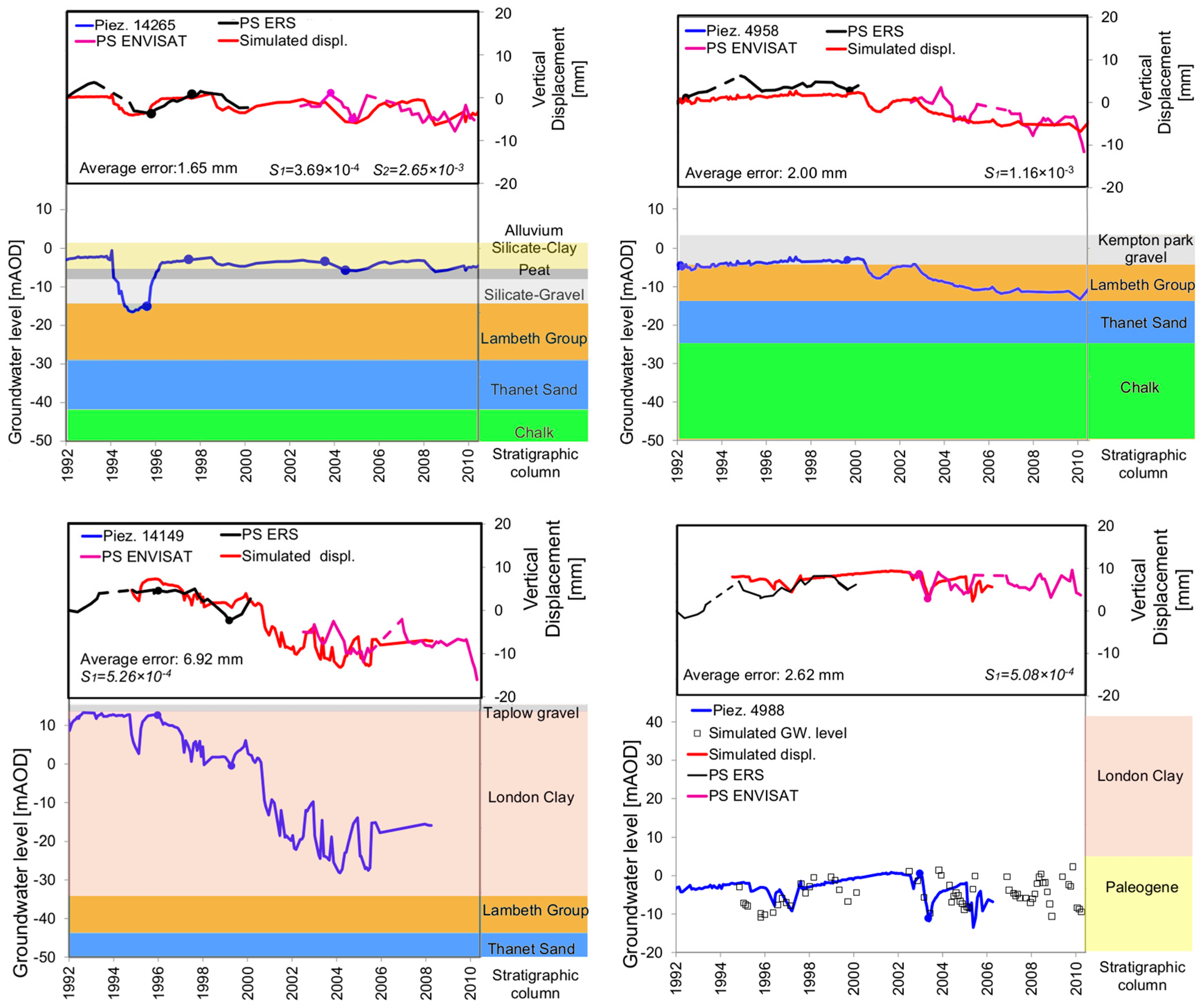
3.3. Time Series Support for Modelling of Land Subsidence: The London Basin Test Case

Principal component analysis (PCA) was performed using ERS-1/2 and ENVISAT data, in order to find the spatio-temporal deformation pattern across the London Basin. Figure 12 shows that both datasets are characterized by two principal components of ground motion. The first component represents land subsidence and the second one is an uplift trend. ERS-1/2 dataset shows that 91.6% of the variance is explained by the first component of motion and 4.4% by the second one. The variance is explained be the first and second components of motion (82.5% and 5.4%, respectively) using the ENVISAT data. Such comparisons were performed between the distribution of PC1 and PC2 with the areas of observed natural and anthropogenic geohazards mapped using the PanGeo procedure [26]. These areas were identified combining the same A-DInSAR datasets with geological data [53]. The distribution of PC1 detected using ERS-1/2 and ENVISAT data matches with natural ground movements, such as those due to compressible ground, and anthropogenic ground instability, such as that due to underground construction. The distribution of the PC2 detected using ERS-1/2 and ENVISAT data corresponds to areas where groundwater rise was previously observed [53] and areas in which causes of uplift are unknown [53], whereas geohazard areas due to tectonic uplift movements characterized by low confidence levels [53] do not show evident correlation with the PC2 trend.
A-DInSAR time series were used to simulate the acceleration and deceleration of the displacement in response to the changes in the piezometric level across the London Basin. Figure 13 shows the simulated displacements at four piezometers in order to represent the main responses to hydraulic head changes. These are obtained by using the groundwater level data and the estimated storage coefficients as inputs to Equation (2).
In the North London Basin, when the Chalk is confined by the London Clay, the hydraulic head change of 11.50 m coincides with approximately 5.85 mm of surface displacement (Figure 13; piezometer 4988). In the Central London Basin, temporary transition of the water table across the units was detected (Figure 13; piezometer 14265). In this regard, two different storage coefficients were evaluated for the different aquifer conditions in the periods 01 February 1996 to 12 December 1997 and 14 January 2004 to 13 December 2004 for the confined and semi-confined conditions, respectively. The semi-confined conditions in the Lambeth group were observed at piezometer 4958. The hydraulic head change of 2.45 m coincides with approximately 2.85 mm of surface displacement. In the South London Basin, the aquifer is confined by thicker deposits of the London Clay and lower values of the storage coefficient were observed. A hydraulic head change of 13.16 m produces around 6.92 mm of surface displacement (Figure 13; piezometer 14149). The absolute average difference error between the simulated and A-DInSAR time series was also estimated.
The use of A-DInSAR time series for the modelling has allowed finding a correlation between the derived storage coefficient and the aquifer condition. Indeed, where the Chalk is confined by the London Clay the storage coefficient is of the order of 1 × 10⁻⁴, whilst where overlain by the Lambeth Group and semi-confined conditions are expected to exist, the storage is higher, typically 1 × 10⁻³, revealing the additional storage provided by sand-rich horizons in the Lambeth Group.
It is noteworthy how another benefit provided by the use of the simulated displacements is the filling of the temporal gap (approximately two years) between the ERS and ENVISAT data. The ENVISAT ground motion time series in Figure 13 were indeed adjusted for the position of the ground on 13 December 2002 to match with the modelled ground motion time series based on the ERS data. A vertical displacement of −5 mm was estimated for piezometer 14149 and −2 mm for piezometer 14265.
Furthermore, Equation (3) was applied in order to simulate the hydraulic head changes based on the observed ground motion at piezometer 4988 (Figure 13). The results show that the A-DInSAR time series could be used to simulate groundwater level changes following this innovative approach. It is worth noting that the relative error between the simulated hydraulic head changes and the measured groundwater level variations using time series acquired by the ERS and ENVISAT sensors is 25% of the hydraulic head change. The frequency of measurements between the displacement and piezometric time series is about 4–6 measurements per year versus 12 measurements per year. Therefore, the difference in the temporal sampling of these measurements could be influencing the error of the model.

4. Conclusions

This work aimed at exploiting the support of A-DInSAR time series for different facets of land subsidence mechanism assessment, starting from detection, up to the characterization and 1-D modelling. The main advantages and limitations of the A-DInSAR time series from an end-user point of view are discussed through three well-studied test sites: the Oltrepo Pavese (Po Plain, in Italy), the Alto Guadalentín (Spain), and the London Basin (UK). In particular, time series analysis was carried out in the Oltrepo Pavese for the detection of the ground motion areas. The time series support for the characterization and the modelling of land subsidence mechanisms was assessed, respectively, in the Alto Guadalentín Basin and in the London Basin.
Although various methodologies were implemented to map the ground motion areas using the average velocity detected by A-DInSAR data [25,26,27,28,29,30], the use of the time series for the detection of ground motion areas is still not a common practice in the scientific community. The main advantage of A-DInSAR time series for the detection of the ground motion areas is the unprecedented mapping of different deformational behaviors, such as in the case of the Oltrepo Pavese. By exploiting the A-DInSAR time series, the distribution of the areas affected by linear, non-linear, and seasonal movements was assessed. Furthermore, two approaches were applied to detect ground motion areas in order to give insight into the obtained results using the time series and the average velocity. Long-term movements detected using principal component analysis (PCA) are consistent with the results obtained using the average velocity. Otherwise, additional seasonal trends are observed using only PCA.
For the test site of the Alto Guadalentín Basin, PCA analysis was performed using the ERS and ENVISAT, ALOS, and COSMO-SkyMed data. The different datasets show that the Alto Guadalentín Basin is characterized by one component of motion that displays a land subsidence trend. Furthermore, the integrated analysis of A-DInSAR time series acquired by multi-temporal sensors allowed the characterization of the long-term subsidence. The collection of A-DInSAR time series acquired by multi-temporal sensors provided valuable information about the typology of aquifer deformation. Indeed, the use in conjunction of multi-sensor A-DInSAR data prove to be fundamental for the reconstruction of long-term evolution of land subsidence due to groundwater management, as in the case of the history of the Alto Guadalentín aquifer exploitation, confirming the potentials of the back-monitoring approach. Furthermore, the analysis of time series carried out for the Alto Guadalentín Basin has allowed the detection of transient aquifer deformation and inelastic aquifer deformation, not otherwise detectable by exploiting the average velocity. Further consideration to be taken into account for time series acquired by different sensors is how to fill the temporal gap between the datasets. With regard to this issue, the linear velocity was assumed in the temporal gaps (11 months) of the ALOS PALSAR and COSMO-SkyMed datasets. The results are consistent with the measurements obtained by two GPS stations.
Finally, PCA analysis was also performed for the ERS-1/2 and ENVISAT data available for the London Basin. Two components of ground motion were recognized, being related to land subsidence and uplift trends. PCA results are consistent with the areas delineated using the PanGeo procedure. Only geohazard areas due to tectonic uplift movements with low confidence levels show no evident correlation with PC2.
Furthermore, changes, such as acceleration and deceleration in the displacement rates in the London Basin, were simulated by calibrating a 1-D model using A-DInSAR time series. The modelling also has the benefit of filling the temporal gap between ERS and ENVISAT time series (about two years). A-DInSAR time series were also used as input for an inverse model in order to simulate the hydraulic head. This approach could be used to exploit A-DInSAR time series for groundwater level change monitoring in areas where no observation boreholes are available. Thus, we believe that new opportunities and perspectives will emerge for the detection and interpretation of subsiding phenomena using A-DInSAR time series provided by improved acquisition frequency, achievable through new high-resolution SAR satellite sensors, such as COSMO-SkyMed and Sentinel-1 constellations, thanks to the shorter revisiting time.
More widely, the findings of this work confirmed that time series represent an added value for a variety of activities in the framework of land subsidence mitigation and management. These observations have significant implications for similar studies in other geological contexts.

Acknowledgments

Groundwater level data for the London Basin were provided by the Environment Agency (Licence No. A2719; non-commercial use), and the ERS and ENVISAT PS data via the EC FP7 PanGeo project. Francesca Cigna and Stephanie Bricker publish with the permission of the Executive Director of BGS. Part of this work was supported by the Spanish Ministry of Economy and Competitiveness and EU FEDER funds under projects TIN2014-55413- C2-2-P and ESP2013-47780-C2-2-R.

Author Contributions

Roberta Bonì carried out this study and wrote this paper in the framework of her Ph.D. project at the University of Pavia, and during her research visits to the Geological Survey of Spain (IGME) in January–March 2015, and the British Geological Survey (BGS) in June–September 2015. Claudia Meisina provided guidance and support throughout the research process for the three case histories. Francesca Cigna supervised Roberta Bonì during her visit at BGS and revised the manuscript. Davide Notti supported the analysis of the A-DInSAR time series for the Oltrepo Pavese and Alto Guadalentín Basin. Stephanie Bricker provided support for the characterization of hydrogeological properties of the Chalk aquifer. Harry McCormack processed ERS-1/2 and ENVISAT data for the London Basin. Gerardo Herrera supervised Roberta Bonì during her visit to IGME. Roberto Tomás provided support to understand the land subsidence mechanism in the Alto Guadalentín Basin. Marta Béjar-Pizarro contributed analyses of the SAR data for the Alto Guadalentín Basin. Joaquin Mulas supported the analysis of the geological data about the Alto Guadalentín Basin. Pablo Ezquerro supported the analysis of the land subsidence in the Alto Guadalentín Basin. All authors co-wrote and reviewed the manuscript.

Conflicts of Interest

The authors declare no conflict of interest.

References

  1. Holzer, T.L.; Galloway, D.L. Impacts of land subsidence caused by withdrawal of underground fluids in the United States. Rev. Eng. Geol. 2005, 16, 87–99. [Google Scholar] [CrossRef]
  2. Abidin, H.Z.; Andreas, H.; Gumilar, I.; Sidiq, T.P.; Gamal, M. Environmental Impacts of Land Subsidence in Urban Areas of Indonesia. In Proceedings of the FIG Working Week 2015, TS 3—Positioning and Measurement, Sofia, Bulgaria, 17–21 May 2015. [Google Scholar]
  3. Syvitski, J.; Higgins, S. Going under: The world’s sinking deltas. New Sci. 2012, 216, 40–43. [Google Scholar] [CrossRef]
  4. Galloway, D.; Jones, D.R.; Ingebritsen, S.E. Land Subsidence in the United States; US Geological Survey: Reston, VA, USA, 1999; p. 177.
  5. Cigna, F.; Osmanoğlu, B.; Cabral-Cano, E.; Dixon, T.H.; Ávila-Olivera, J.A.; Gardũno-Monroy, V.H.; DeMets, C.; Wdowinski, S. Monitoring land subsidence and its induced geological hazard with Synthetic Aperture Radar Interferometry: A case study in Morelia, Mexico. Remote Sens. Environ. 2012, 117, 146–161. [Google Scholar] [CrossRef]
  6. Bozzano, F.; Esposito, C.; Franchi, S.; Mazzanti, P.; Perissin, D.; Rocca, A.; Romano, E. Understanding the subsidence process of a quaternary plain by combining geological and hydrogeological modelling with satellite InSAR data: The Acque Albule Plain case study. Remote Sens. Environ. 2015, 168, 219–238. [Google Scholar] [CrossRef]
  7. Jones, C.E.; An, K.; Blom, R.G.; Kent, J.D.; Ivins, E.R.; Bekaert, D. Anthropogenic and geologic influences on subsidence in the vicinity of New Orleans, Louisiana. J. Geophys. Res. Solid Earth 2016, 121, 3867–3887. [Google Scholar] [CrossRef]
  8. Herrera, G.; Fernández, J.A.; Tomás, R.; Cooksley, G.; Mulas, J. Advanced interpretation of subsidence in Murcia (SE Spain) using A-DInSAR data-modelling and validation. Nat. Hazards Earth Syst. Sci. 2009, 9, 647. [Google Scholar] [CrossRef]
  9. Crosetto, M.; Monserrat, O.; Cuevas-González, M.; Devanthéry, N.; Crippa, B. Persistent scatterer interferometry: A review. ISPRS J. Photogramm. Remote Sens. 2016, 115, 78–89. [Google Scholar] [CrossRef]
  10. Ferretti, A.; Fumagalli, A.; Novali, F.; Prati, C.; Rocca, F.; Rucci, A. A new algorithm for processing interferometric data-stacks: SqueeSAR. IEEE Trans. Geosci. Remote Sens. 2011, 49, 3460–3470. [Google Scholar] [CrossRef]
  11. Kampes, B.M.; Hanssen, R.F.; Perski, Z. Radar interferometry with public domain tools. In Proceedings of the FRINGE 2003 Workshop, Frascati, Italy, 1–5 December 2003. [Google Scholar]
  12. Arnaud, A.; Adam, N.; Hanssen, R.; Inglada, J.; Duro, J.; Closa, J.; Eineder, M. ASAR ERS Interferometric phase continuity. In Proceedings of the International Geoscience and Remote Sensing Symposium, Toulouse, France, 21–25 July 2003. [Google Scholar]
  13. Berardino, P.; Fornaro, G.; Lanari, R.; Sansosti, E. A new algorithm for surface deformation monitoring based on small baseline differential SAR interferograms. IEEE Trans. Geosci. Remote Sens. 2002, 40, 2375–2383. [Google Scholar] [CrossRef]
  14. Duro, J.; Closa, J.; Biescas, E.; Crosetto, M.; Arnaud, A. High Resolution Differential Interferometry using time series of ERS and ENVISAT SAR data. In Proceedings of the 6th Geomatic Week Conference, Barcelona, Spain, February 2005; Available online: https://pdfs.semanticscholar.org/d4bc/b3461ddb06da0704815bb40d815d780c8eb8.pdf (accessed on 10 April 2017).
  15. Hooper, A. A multi-temporal InSAR method incorporating both persistent scatterer and small baseline approaches. Geophys. Res. Lett. 2008, 35, L16302. [Google Scholar] [CrossRef]
  16. US National Research Council. Mitigating Losses from Land Subsidence in the United States; National Academy Press: Washington, DC, USA, 1991.
  17. González, P.J.; Fernández, J. Drought-driven transient aquifer compaction imaged using multitemporal satellite radar interferometry. Geology 2011, 39, 551–554. [Google Scholar] [CrossRef]
  18. Meisina, C.; Zucca, F.; Fossati, D.; Ceriani, M.; Allievi, J. Ground deformation monitoring by using the permanent scatterers technique: The example of the Oltrepo Pavese (Lombardia, Italy). Eng. Geol. 2006, 88, 240–259. [Google Scholar] [CrossRef]
  19. Brambilla, G. Prime considerazioni cronologico-ambientali sulle filliti del Miocene superiore di Portalbera (Pavia-Italia settentrionale). In Nuove Ricerche Archeologiche in Provincia di Pavia, Proceedings of the Convegno di Casteggio, Casteggio, Italy, 14 October 1990; Civico Museo Archeologico di Casteggio e dell’Oltrepò Pavese: Casteggio, Italy, 1992; pp. 109–113. (In Italian) [Google Scholar]
  20. Pellegrini, L.; Vercesi, P.L. Considerazioni morfotettoniche sulla zona a sud del Po tra Voghera (PV) e Sarmato (PC). Atti Tic. Sci. Terra 1995, 38, 95–118. (In Italian) [Google Scholar]
  21. Cavanna, F.; Marchetti, G.; Vercesi, P.L. Idrogeomorfologia e Insediamenti a Rischio Ambientale. Il Caso Della Pianura Dell’Oltrepò Pavese e del Relativo Margine Collinare; Ricerche & Risultati, Valorizzazione dei progetti di ricerca 1994/97; Fondazione Lombardia Ambiente; Isabel Litografia: Gessate, Italy, 1998; pp. 14–72. (In Italian) [Google Scholar]
  22. Pilla, G.; Sacchi, E.; Ciancetti, G. Studio idrogeologico, idrochimico ed isotopico delle acque sotterranee del settore di pianura dell’Oltrepò Pavese (Pianura lombarda meridionale). G. Geol. Appl. 2007, 5, 59–74. (In Italian) [Google Scholar]
  23. Boni, A.; Boni, P.; Peloso, G.F.; Gervasoni, S. Dati sulla neotettonica del foglio di Pavia (59) e di parte dei fogli voghera (71) ed alessandria (70). CNRPF Geodin. Pubbl. 1980, 356, 1199–1223. (In Italian) [Google Scholar]
  24. Meisina, C. Engineering geological mapping for urban areas of the Oltrepo Pavese plain (Northern Italy). In Proceedings of the 10th Congress of the International Association for Engineering Geology and the Environment (IAEG), Nottingham, UK, 6–10 September 2006. [Google Scholar]
  25. Meisina, C.; Zucca, F.; Notti, D.; Colombo, A.; Cucchi, A.; Savio, G.; Giannico, C.; Bianchi, M. Geological interpretation of PSInSAR data at regional scale. Sensors 2008, 8, 7469–7492. [Google Scholar] [CrossRef] [PubMed]
  26. Bateson, L.; Cuevas, M.; Crosetto, M.; Cigna, F.; Schijf, M.; Evans, H. PANGEO: Enabling Access to Geological Information in Support of GMES: Deliverable 3.5 Production Manual. version 1. 2012. Available online: http://nora.nerc.ac.uk/19289/ (accessed on 10 April 2017).
  27. Bianchini, S.; Cigna, F.; Righini, G.; Proietti, C.; Casagli, N. Landslide hotspot mapping by means of persistent scatterer interferometry. Environ. Earth Sci. 2012, 67, 1155–1172. [Google Scholar] [CrossRef]
  28. Lu, P.; Casagli, N.; Catani, F.; Tofani, V. Persistent Scatterers Interferometry Hotspot and Cluster Analysis (PSI-HCA) for detection of extremely slow-moving landslides. Int. J. Remote Sens. 2012, 33, 466–489. [Google Scholar] [CrossRef]
  29. Peduto, D.; Cascini, L.; Arena, L.; Ferlisi, S.; Fornaro, G.; Reale, D. A general framework and related procedures for multiscale analyses of DInSAR data in subsiding urban areas. ISPRS J. Photogramm. Remote Sens. 2015, 105, 186–210. [Google Scholar] [CrossRef]
  30. Di Martire, D.; Novellino, A.; Ramondini, M.; Calcaterra, D. A-differential synthetic aperture radar interferometry analysis of a Deep Seated Gravitational Slope Deformation occurring at Bisaccia (Italy). Sci. Total Environ. 2016, 550, 556–573. [Google Scholar] [CrossRef] [PubMed]
  31. Bonì, R.; Pilla, G.; Meisina, C. Methodology for Detection and Interpretation of Land subsidence Areas with the A-DInSAR Time Series Analysis. Remote Sens. 2016, 8, 686. [Google Scholar] [CrossRef]
  32. Bourgois, J.; Mauffret, A.; Ammar, A.; Demnati, A. Multichannel seismic data imaging of inversion tectonics of the Alboran Ridge (Western Mediterranean Sea). Geo-Mar. Lett. 1992, 12, 117–122. [Google Scholar] [CrossRef]
  33. Martınez-Dıaz, J.J. Stress field variation related to fault interaction in a reverse oblique-slip fault: The Alhama deMurcia fault, Betic Cordillera, Spain. Tectonophysics 2002, 356, 291–305. [Google Scholar] [CrossRef]
  34. Instituto Geológico y Minero de España (IGME). Mapa Geologico de España, 1:50.000, Sheet Lorca (953); Servicio de Publicaciones Ministerio de Industria: Madrid, Spain, 1981. (In Spanish)
  35. Cerón, J.C.; Pulido-Bosch, A. Groundwater problems resulting from CO2 pollution and overexploitation in Alto Guadalentín aquifer (Murcia, Spain). Environ. Geol. 1996, 28, 223–228. [Google Scholar]
  36. Confederación Hidrográfica del Segura (CHS). Plan especial ante situaciones de alerta y eventual sequia en la cuenca del Segura: Confederacion hidrografica del Segura. Technical Report. 1996. (In Spanish). Available online: https://www.chsegura.es/chs/cuenca/sequias/pes/eeapes.html (accessed on 11 April 2017).
  37. Martín, V.J.M.; Espinosa, G.J.S.; Pérez, R.A. Mapa geológico de España: E. 1:50,000; Servicio de Publicaciones, Ministerio de Industria y Energía, Instituto geológico y minero de España (IGME): Madrid, Spain, 1973.
  38. González, P.J.; Fernández, J. Error estimation in multitemporal InSAR deformation time series, with application to Lanzarote, Canary Islands. J. Geophys. Res. 2011, 116, B10404. [Google Scholar] [CrossRef]
  39. Bonì, R.; Herrera, G.; Meisina, C.; Notti, D.; Béjar-Pizarro, M.; Zucca, F.; González, P.J.; Palano, M.; Tomás, R.; Fernández, J.; et al. Twenty-year advanced DInSAR analysis of severe land subsidence: The Alto Guadalentín Basin (Spain) case study. Eng. Geol. 2015, 198, 40–52. [Google Scholar] [CrossRef]
  40. Zhang, Y.; Xue, Y.-Q.; Wu, J.-C.; Ye, S.-J.; Wei, Z.-W.; Li, Q.-F.; Yu, J. Characteristics of aquifer system deformation in the Southern Yangtse Delta, China. Eng. Geol. 2007, 90, 160–173. [Google Scholar] [CrossRef]
  41. Royse, K.R.; de Freitas, M.; Burgess, W.G.; Cosgrove, J.; Ghail, R.C.; Gibbard, P.; King, C.; Lawrence, U.; Mortimore, R.N.; Owen, H.G.; et al. Geology of London, UK. Proc. Geol. Assoc. 2012, 123, 22–45. [Google Scholar] [CrossRef]
  42. Ford, J.R.; Mathers, S.J.; Royse, K.R.; Aldiss, D.T.; Morgan, D.J.R. Geological 3D modelling: Scientific discovery and enhanced understanding of the subsurface, with examples from the UK. Z. Dtsch. Ges. Geowiss. 2010, 161, 205–218. [Google Scholar] [CrossRef]
  43. Mathers, S.J.; Burke, H.F.; Terrington, R.L.; Thorpe, S.; Dearden, R.A.; Williamson, J.P.; Ford, J.R. A geological model of London and the Thames Valley, southeast England. Proc. Geol. Assoc. 2014, 125, 373–382. [Google Scholar] [CrossRef]
  44. Ellison, R.A.; Woods, M.A.; Allen, D.J.; Forster, A.; Pharaoh, T.C.; King, C. Geology of London: Special Memoir for 1:50,000 Geological Sheets 256 (North London), 257 (Romford), 270 (South London), and 271 (Dartford) (England and Wales); British Geological Survey: Nottingham, UK, 2004.
  45. Sumbler, M.G. British Regional Geology: London and the Thames Valley, 4th ed.; HMSO for the British Geological Survey: London, UK, 1996. [Google Scholar]
  46. Jones, M.A.; Hughes, A.G.; Jackson, C.R.; Van Wonderen, J.J. Groundwater resource modelling for public water supply management in London. Geol. Soc. Lond. Spec. Publ. 2012, 364, 99–111. [Google Scholar] [CrossRef]
  47. Fry, V.A. Lessons from London: Regulation of open-loop ground source heat pumps in central London. Q. J. Eng. Geol. Hydrogeol. 2009, 42, 325–334. [Google Scholar] [CrossRef]
  48. Bloomfield, J.P.; Bricker, S.H.; Newell, A.J. Some relationships between lithology, basin form and hydrology: A case study from the Thames basin, UK. Hydrol. Process. 2011, 25, 2518–2530. [Google Scholar] [CrossRef]
  49. O’Shea, M.J.; Sage, R. Aquifer recharge: An operational drought-management strategy in North London. Water Environ. J. 1999, 13, 400–405. [Google Scholar] [CrossRef]
  50. O’Shea, M.J.; Baxter, K.M.; Charalambous, A.N. The hydrogeology of the Enfield-Haringey artificial recharge scheme, north London. Q. J. Eng. Geol. Hydrogeol. 1995, 28 (Suppl. 2), S115–S129. [Google Scholar] [CrossRef]
  51. Bonì, R.; Cigna, F.; Bricker, S.; Meisina, C.; McCormack, H. Characterisation of hydraulic head changes and aquifer properties in the London Basin using Persistent Scatterer Interferometry land subsidence data. J. Hydrol. 2016, 540, 835–849. [Google Scholar] [CrossRef]
  52. Werner, C.; Wegmüller, U.; Wiesmann, A.; Strozzi, T. Interferometric point target analysis with JERS-1 L-band SAR data. In Proceedings of the IEEE International Geoscience and Remote Sensing Symposium, IGARSS 2003, Toulouse, France, 21–25 July 2003; Volume 7, pp. 4359–4361. [Google Scholar]
  53. Cigna, F.; Jordan, H.; Bateson, L.; McCormack, H.; Roberts, C. Natural and anthropogenic geohazards in greater London observed from geological and ERS-1/2 and ENVISAT persistent scatterers land subsidence data: Results from the EC FP7-SPACE PanGeo Project. Pure Appl. Geophys. 2015, 172, 2965–2995. [Google Scholar] [CrossRef]
  54. Chaussard, E.; Bürgmann, R.; Shirzaei, M.; Fielding, E.J.; Baker, B. Predictability of hydraulic head changes and characterization of aquifer-system and fault properties from InSAR-derived ground deformation. J. Geophys. Res. Solid Earth 2014, 119, 6572–6590. [Google Scholar] [CrossRef]
  55. Hoffmann, J.; Galloway, D.L.; Zebker, H.A. Inverse modelling of interbed storage parameters using land subsidence observations, Antelope Valley, California. Water Resour. Res. 2003, 39. [Google Scholar] [CrossRef]
  56. Calderhead, A.I.; Therrien, R.; Rivera, A.; Martel, R.; Garfias, J. Simulating pumping-induced regional land subsidence with the use of InSAR and field data in the Toluca Valley, Mexico. Adv. Water Resour. 2011, 34, 83–97. [Google Scholar] [CrossRef]
  57. Teatini, P.; Castelletto, N.; Ferronato, M.; Gambolati, G.; Janna, C.; Cairo, E.; Marzorati, D.; Colombo, D.; Ferretti, A.; Bagliani, A.; et al. Geomechanical response to seasonal gas storage in depleted reservoirs: A case study in the Po River basin, Italy. J. Geophys. Res. Earth Surf. 2011, 116. [Google Scholar] [CrossRef]
  58. Hoffmann, J.; Zebker, H.A.; Galloway, D.L.; Amelung, F. Seasonal subsidence and rebound in Las Vegas Valley, Nevada, observed by Synthetic Aperture Radar Interferometry. Water Resour. Res. 2001, 37, 1551–1566. [Google Scholar] [CrossRef]
  59. Tomás, R.; Herrera, G.; Delgado, J.; Lopez-Sanchez, J.M.; Mallorquí, J.J.; Mulas, J. A ground subsidence study based on DInSAR data: Calibration of soil parameters and subsidence prediction in Murcia City (Spain). Eng. Geol. 2010, 111, 19–30. [Google Scholar] [CrossRef]
  60. Ezquerro, P.; Herrera, G.; Marchamalo, M.; Tomás, R.; Béjar-Pizarro, M.; Martínez, R. A quasi-elastic aquifer deformational behavior: Madrid aquifer case study. J. Hydrol. 2014, 519, 1192–1204. [Google Scholar] [CrossRef]
  61. Benedetti, L.C.; Tapponnier, P.; Gaudemer, Y.; Manighetti, I.; van der Woerd, J. Geomorphic evidence for an emergent active thrust along the edge of the Po Plain: The Broni-Stradella fault. J. Geophys. Res. Solid Earth 2003, 108. [Google Scholar] [CrossRef]
  62. Meisina, C. Light buildings on swelling/shrinking soils: Case histories from Oltrepo Pavese (north-western Italy). Int. Conf. Probl. Soils 2003, 2, 28–30. [Google Scholar]
Figure 1. Location of the study areas.
Geosciences 07 00025 g001
Figure 2. Engineering geological map of the plain area of the Oltrepo Pavese, modified from [24].
Geosciences 07 00025 g002
Figure 3. (a) Line of sight (LOS) velocity measured by the use of ERS-1/2 descending data (time interval from 1992 to 2000) and (b) RADARSAT ascending data (time interval from 2003 to 2010), modified from [31]. The reference points are also reported.
Geosciences 07 00025 g003
Figure 4. Geological setting of the Alto Guadalentín Basin modified from [37]. The localization of the Global Positioning System (GPS) stations, called Lor1 and Lorc, is also reported.
Geosciences 07 00025 g004
Figure 5. (a) Vertical velocity (Vert. vel.) measured by the use of ERS and ENVISAT data (time interval from 1992 to 2007); (b) ALOS PALSAR (time interval from 2007 to 2010); and (c) COSMO-SkyMed (time interval from 2011 to 2012).
Geosciences 07 00025 g005
Figure 6. Geological setting of London Basin, modified from [51]. Geological materials © NERC 2016. All rights reserved. British National Grid. Projection: Transverse Mercator. Datum: OSGB 1936. The localization of the piezometers is also reported.
Geosciences 07 00025 g006
Figure 7. (a) Vertical velocity (Vert. vel.) measured by the use of ERS (time interval from 1992 to 2000) and (b) ENVISAT (ENV.) data (time interval from 2002 to 2010), overlapped onto shaded relief of NEXTMap® DTM at 50 m resolution; modified from [53]. Reference points for each dataset are also reported. ERS-1/2 and ENVISAT PSI data © CGG NPA Satellite Mapping. NEXTMap® Britain © 2003, Intermap Technologies Inc., All rights reserved.
Geosciences 07 00025 g007
Figure 8. Ground motion areas detected using PC1, PC2, and PC3, and non-linear PS-DS of the ERS-1/2 descending and Radarsat ascending data overlapped on the engineering geological units. Time series (TS) of the deformational behavior detected at Voghera, Stradella–Monteacuto, Casei Gerola, and Codevilla are also reported. For Codevilla, TS were compared with effective rainfall measured at the Voghera weather station.
Geosciences 07 00025 g008
Figure 9. Anomalous areas detected using the average velocity [25] overlapped on the engineering geological units.
Geosciences 07 00025 g009aGeosciences 07 00025 g009b
Figure 10. Principal component (PC) score maps of ERS and ENVISAT, ALOS, and COSMO-SkyMed data. For each dataset, the eigenvector value and the percentage of explained variance are also reported.
Geosciences 07 00025 g010
Figure 11. Cumulated displacement from 1992 to 2012 and cross-comparison of the piezometric level variations from 1975 to 2012 (black and pink lines) at the different piezometers (P1, P2, P3a, P3b, P4a, P4b, and P5) with the displacement time series detected by the satellite sensors (blue, red, and yellow lines). For some piezometers the lithological column is reported. The dotted line is the ground level. Piez. stands for piezometer.
Geosciences 07 00025 g011
Figure 12. Principal component (PC) score maps of the ERS-1/2 and ENVISAT data using the first and the second component of the movements (PC1, PC2). For each dataset, the eigenvector value and the percentage of the explained variance are also reported.
Geosciences 07 00025 g012
Figure 13. Comparison of A-DInSAR time series for 1992–2000 (PS ERS) and 2002–2010 (PS ENVISAT) and simulated displacements (mm) with the groundwater level variations (m) (modified from [51]). In addition, the stratigraphic column is represented. The dots represent the start and the end of the calibration period for the simulation. Piezometer localization is shown in Figure 6. For piezometer 4988, the simulated groundwater (GW) level is also reported. Groundwater level data © Environment Agency copyright and/or database rights 2015. All rights reserved.
Geosciences 07 00025 g013
Table 1. Test case characteristics and available A-DInSAR data.
Test CaseSAR DataSensorProcessing TechniqueTime SpanType of Land SubsidenceArea (km2)
Oltrepo Pavese (Italy) ERS-1/2C-bandSqueeSAR™1992–2000Natural and anthropic causes440
RADARSAT-1C-bandSqueeSAR™2003–2010
Alto Guadalentín Basin (Spain)ERS-1/2C-bandStaMPS1992–2000Anthropogenic subsidence due to groundwater extraction277
ENVISATC-bandStaMPS2003–2007
ALOS-PALSARL-bandSPN2007–2010
COSMO-SkyMedX-bandSPN2011–2012
London Basin (United Kingdom)ERS-1/2C-bandIPTA1992–2000Natural and anthropic causes
ENVISATC-bandIPTA2002–20101360

