Three-Dimensional Geological Model of Quaternary Sediments in Walworth County, Wisconsin, USA

Abstract

A three-dimensional (3D) geologic model was developed for Quaternary deposits in southern Walworth County, WI using Petrel, a software package primarily designed for use in the energy industry. The purpose of this research was to better delineate and characterize the shallow glacial deposits, which include multiple shallow sand and gravel aquifers. The 3D model of Walworth County was constructed using datasets such as the U.S. Geological Survey 30 m digital elevation model (DEM) of land surface, published maps of the regional surficial geology and bedrock topography, and a database of water-well records. Using 3D visualization and interpretation tools, more than 1400 lithostratigraphic picks were efficiently interpreted amongst 725 well records. The final 3D geologic model consisted of six Quaternary lithostratigraphic units and a bedrock horizon as the model base. The Quaternary units include in stratigraphic order from youngest to oldest: the New Berlin Member of the Holy Hill Formation, the Tiskilwa Member of the Zenda Formation, a Sub-Tiskilwa Sand/Gravel unit, the Walworth Formation, a Sub-Walworth Sand/Gravel unit, and a Pre-Illinoisan unit. Compared to previous studies, the results of this study indicate a more detailed distribution, thickness, and interconnectivity between shallow sand and gravel aquifers and their connectivity to shallow bedrock aquifers. This study can also help understand uncertainty within previous local groundwater-flow modeling studies and improve future studies.

1. Introduction

In the northern United States and Canada, Quaternary deposits are being used to meet the growing demand for water resources [1]. Proper management of these resources is improved through building more accurate geologic models [2]. For example, consultants and planners can make better-informed models and decisions, respectively, when addressing long-term water resource needs. Within the last decade, advances in computer technology have facilitated the construction of 3D geologic models. These models can often more clearly show the thickness and distribution of glacial materials [1,3,4] and provide local governments information needed to make educated resource management decisions. For example, there have been successfully conducted studies to construct 3D geologic models for southern Ontario and Quebec.

3D visualization of the shallow subsurface provides more detailed insight that is not available from conventional 2D geological sources. Depending on the availability and density of subsurface geologic data, visualization and analysis of multiple forms of data such as hydrogeology and geophysical data can help show the spatial distribution and interconnectivity of deposits in the shallow subsurface [5,6]. Complexity and variability within sand and gravel aquifer systems, which is sometimes neglected as insignificant in groundwater flow models, may play important roles in controlling local and regional groundwater flow and recharge paths in glacial sediments. 3D geologic mapping of these aquifer systems will provide insight that can aid regional groundwater flow modeling efforts in an area [2]. Hydrogeologic implications from detailed 3D geologic models are significant in the context of regional groundwater flow systems.

In this study, Petrel was used to create a 3D model Quaternary deposits in a portion of southeast Wisconsin. Petrel is a 3D subsurface modeling software that has typically been used for modeling deep hydrocarbon reservoirs in sedimentary bedrock. Glacial sediments are often much less continuous than sedimentary bedrock, but several recent studies have shown that Petrel can effectively be used in glacial settings as well. Hartz et al. [7] used Petrel to model sediment-fill geometries in subglacial tunnel valleys in central Illinois. Carlock [8] successfully used Petrel to build a 3D geologic model and facies model of the Pearl-Ashmore Aquifer in north-central McHenry County, which is just south of the current study area.

2. Geology

The Quaternary deposits of Walworth County have been studied for decades [9,10,11,12,13,14,15,16,17] (Figure 1). The first comprehensive study of the Pleistocene stratigraphy of Wisconsin was completed by Chamberlin [9], and more recently, Syverson et al. [17] developed a reclassification of lithostratigraphy of Pleistocene deposits. More detailed studies in southeastern Wisconsin by Schneider [13] and Gotkowitz and Carter [16] focused on regional geologic history and hydrogeologic context, respectively.

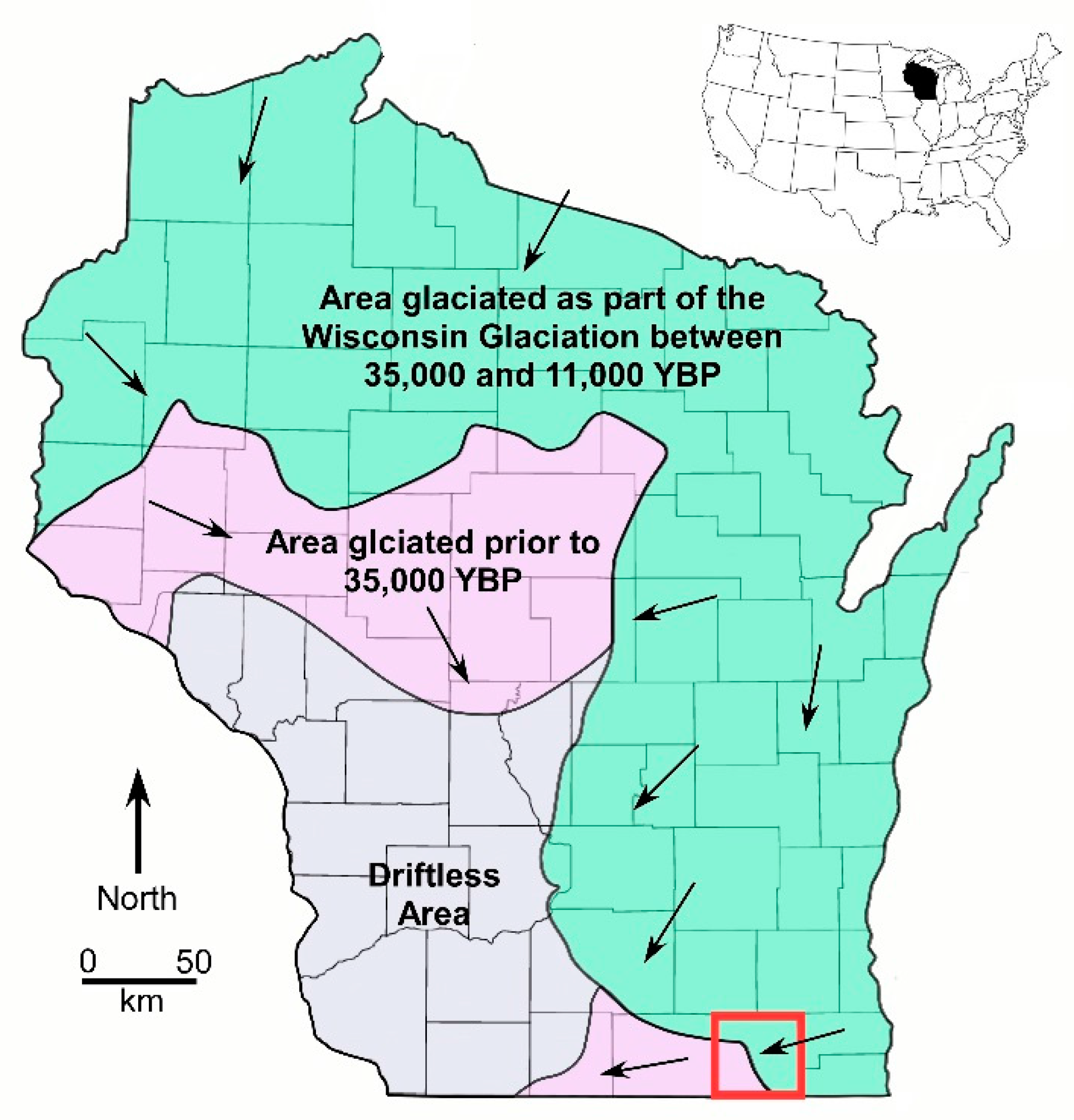
The Quaternary deposits in Walworth County vary from a few tens of meters thick to over 120 m thick. These sediments lay unconformably atop Ordovician and Silurian rocks and locally fill the northern extent of the Troy Bedrock Valley [18], which is incised as much as 100 m. The Quaternary geologic record includes sediments from pre-Illinoian, Illinoisan, and Wisconsinan events [19]. In Walworth County, most of the pre-Illinoisan sediments are poorly known or likely eroded [19]. Illinoisan sediments are more ubiquitous and most often buried by younger sediments, except for the southwest portion of the county, where those sediments are at land surface. The bulk of the surficial deposits and geomorphology in this area are a result of the Wisconsinan glaciation, particularly the Delavan Sublobe, which was the westernmost sublobe of the Lake Michigan Lobe [13,20,21,22,23].

Alden [10] was the first to describe Illinoisan sediments in southeastern Wisconsin (Figure 2), which in Walworth County, are located beyond the extent of the Wisconsin end moraines. In this area, it is a silt-rich, calcareous gray till that is sparsely distributed below the Illinoisan till of the Winnebago (Walworth herein) Formation [14].

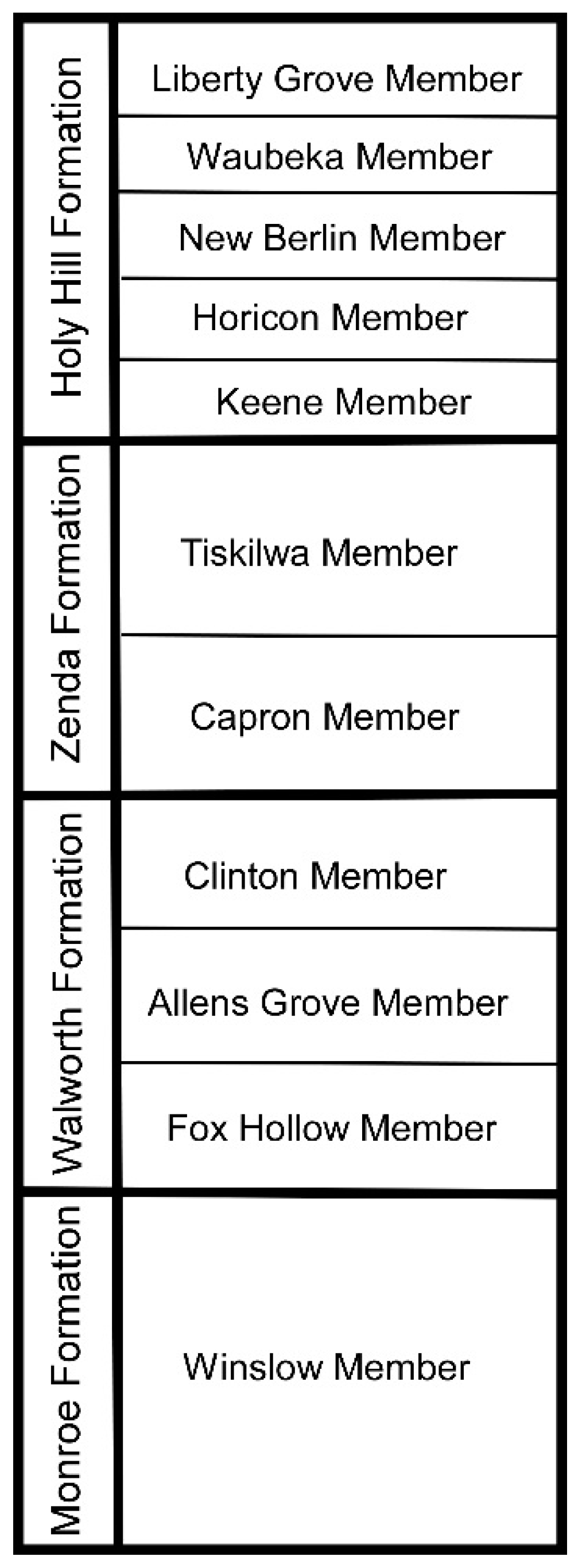
The Walworth Formation consists of the Foxhollow Member, the Allens Grove Member and the Clinton Member. The Foxhollow Member is a gray loam till that has the lowest sand content of the three members and has been found in the Troy Bedrock Valley that trends north–south across western Walworth County. The Allens Grove Member is a pink, sandy loam diamicton. The Clinton Member is the youngest of the three members and is a light brown, sandy till [17].

During the Wisconsin Episode of glaciation, ice advanced and retreated from Walworth County at least two times. Deposits from the Wisconsin Episode are complex assemblages of proglacial and subglacial sediments. In this area, the Zenda Formation consists largely of the Tiskilwa Member, which is a sandy, pink tan clay loam diamicton with sparse sand and gravel lenses. It was deposited by the Delavan Sublobe 18,000–20,000 years before present. It is the most laterally extensive glacial diamicton in the study area. In Walworth County, the Elkhorn Moraine likely consists mainly of the Tiskilwa Formation [10]. The Elkhorn Moraine marks the northwestern extent of the Delavan Sublobe, where the Tiskilwa Formation is overlain by a thin (about 3 m) layer of the New Berlin Member that thickens eastward [17].

The New Berlin Member of the Hoy Hill Formation was deposited 17,000–19,000 years before present. It is a sandy loam diamicton interbedded with sand and gravel lenses and is often underlain by a coarse sand and gravel facies [21].

3. Data Sources

The 3D model of Walworth County was constructed using a variety of surficial and subsurface datasets. These include the USGS 30 m digital elevation model (DEM) of land surface, published maps of the surficial geology [15], and unpublished bedrock topography data throughout of the area, and a database of water-well records provided by the Wisconsin Geological and Natural History Survey (WGNHS). The water well record database in Walworth County is part of a regional database preservation effort in southeast Wisconsin conducted by the WGNHS.

4. Methods

Water well data was originally contained in Microsoft Access databases and other digital data structures. Those sources were used to build 3D visualizations of the water well records using a customized ArcScene tool that was created by the Illinois State Geological Survey (ISGS). Data manipulation and interpretation were then conducted in the 3D environment using standard and customized tools in ESRI’s ArcGIS software. Lastly, a 3D geologic model of the Quaternary deposits in Walworth County was then generated in Petrel.

Water-well records typically have thousands of unique descriptive terms for the various lithological units. To effectively display and interpret those records, the descriptions were standardized into 19 general lithologic categories. A standardized methodology and lithologic dictionary were developed by the ISGS and used in this study. Over 2500 well records were available, and they contained over 9700 lithologic descriptions. Of those descriptions, 96% of them were standardized to the 19 standard descriptions.

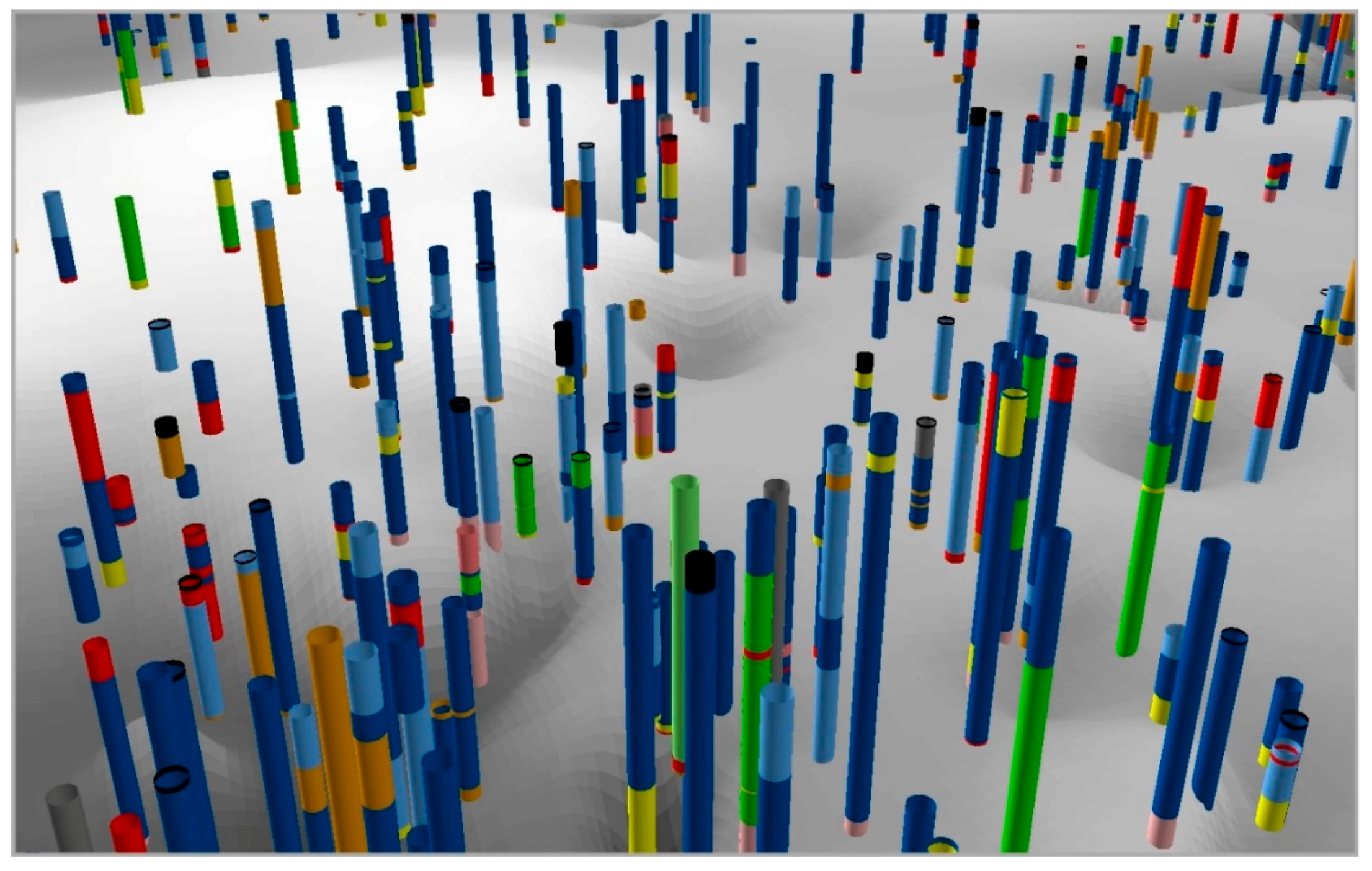
The standardized water well data were then displayed as 3D boreholes using customized tools in ArcGIS, which allowed for interactive 3D visualization, and interpretation of those borehole data. In ArcScene, 3D cylinders were color-coded with respect to lithology as described in Figure 3. “Warm” colors, such as red and orange, indicate coarse-grained sediments, and “cool” colors, such as blue and green, represent fine-grained sediments. The small percentage (4%) of unstandardized lithologies were coded as gray.

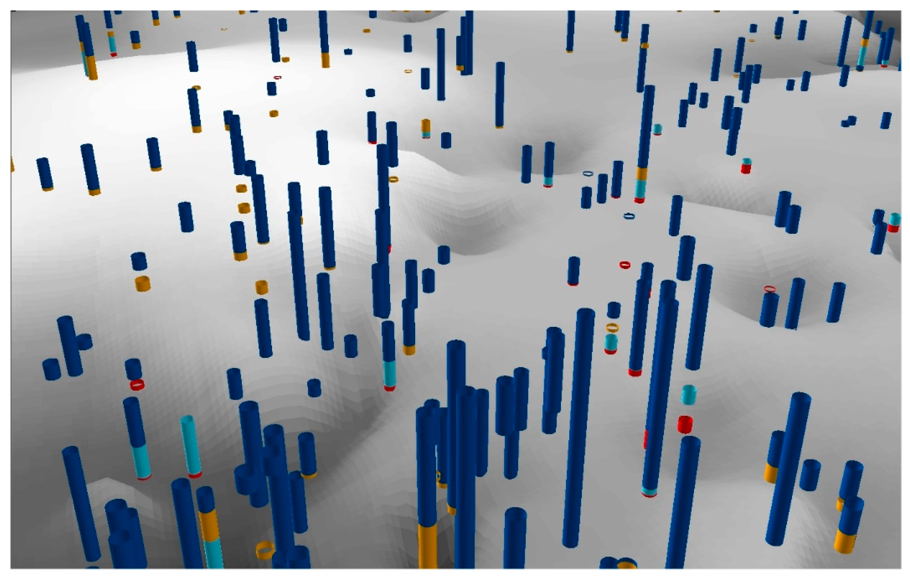
The tops of lithostratigraphic units were interpreted in the 3D ArcGIS environment based on the mappable lithologic correlations between water-well records (Figure 4). Z-values in the water-well records were based on the depth described, and then they were calculated based on the land surface elevation at the given spatial location. Thus, inaccuracies in spatial location and land-surface elevation introduce error in the Z-value calculation. However, those errors are small enough that patterns of subsurface lithology distribution were still mappable.

Because well records often end in the upper part of sand and gravel units and do not penetrate fully through them, the tops of stratigraphic units are most confidently interpreted. Segments of 3D boreholes were selected individually or collectively, and the stratigraphic picks were interpreted based on lithologic characteristics, and then reclassified into 5 geologic units. Those interpretations were then added to the attribute table of the 3D borehole shapefile. The 5 interpreted geologic units were generalized as the New Berlin Member, the Tiskilwa Formation, the Sub-Tiskilwa Sand/Gravel, the Walworth Formation, and the Walworth Sand/Gravel. These stratigraphic picks in the attribute tables were then used as point data for 2D grid interpolation of draft geologic surfaces and contacts. The interpolations integrated the default Topo to Raster options in ArcGIS Spatial Analyst tools. These draft surfaces were usually spatially discontinuous, but they helped with understanding 3D geologic relationships and feasibility of interpretation of the stratigraphy prior to importing the interpreted picks into Petrel.

5. Petrel Three-Dimensional Model

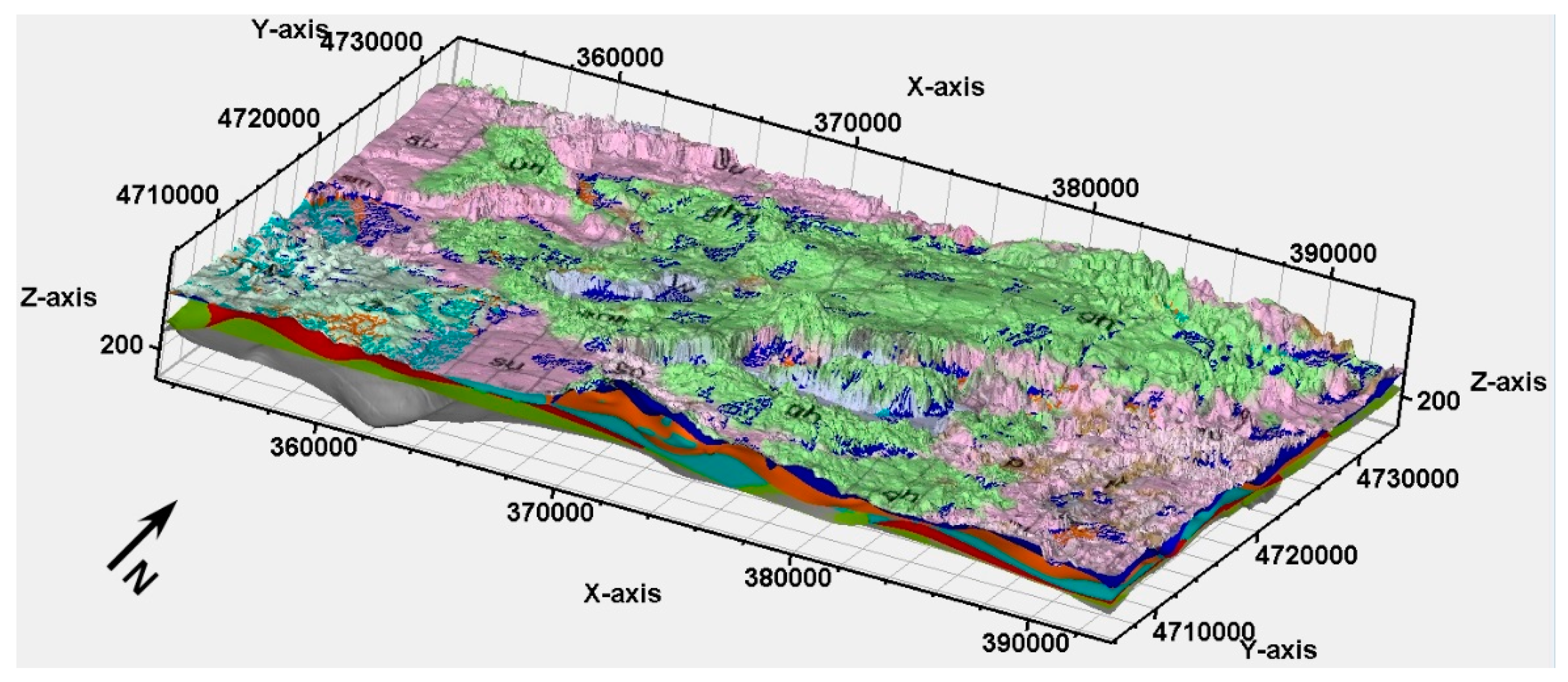
In Petrel a “surface” is a geological surface generated in a 2D grid; a horizon is a geological surface constructed in a 3D grid. Thus, a horizon can have multiple Z values at a single XY location. Surfaces are generated from the imported stratigraphic picks from ArcGIS (Figure 5 and Figure 6) and imported into a model-building module, from which geologic horizons are constructed. Petrel allows for the specification of four different types of stratigraphic horizons: Erosional, Conformable, Discontinuous, or Base. The Erosional horizon truncates those below it and can be used as the top surface or as an intermediate surface. The Conformable horizon will be truncated by any other horizon. A Discontinuous horizon truncates all horizons below it, but horizons above it will lap onto it. Lastly, a Base horizon must be the lowest horizon in the model, such that Conformable horizons will lap onto it and Erosional and Discontinuous horizons will truncate it. For the 3D model in this study, the bedrock was set as a Base horizon, the Pre-Illinois Unit was set as a Conformable horizon and remaining surfaces were set as Erosional horizons.

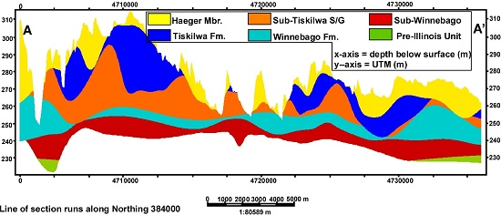
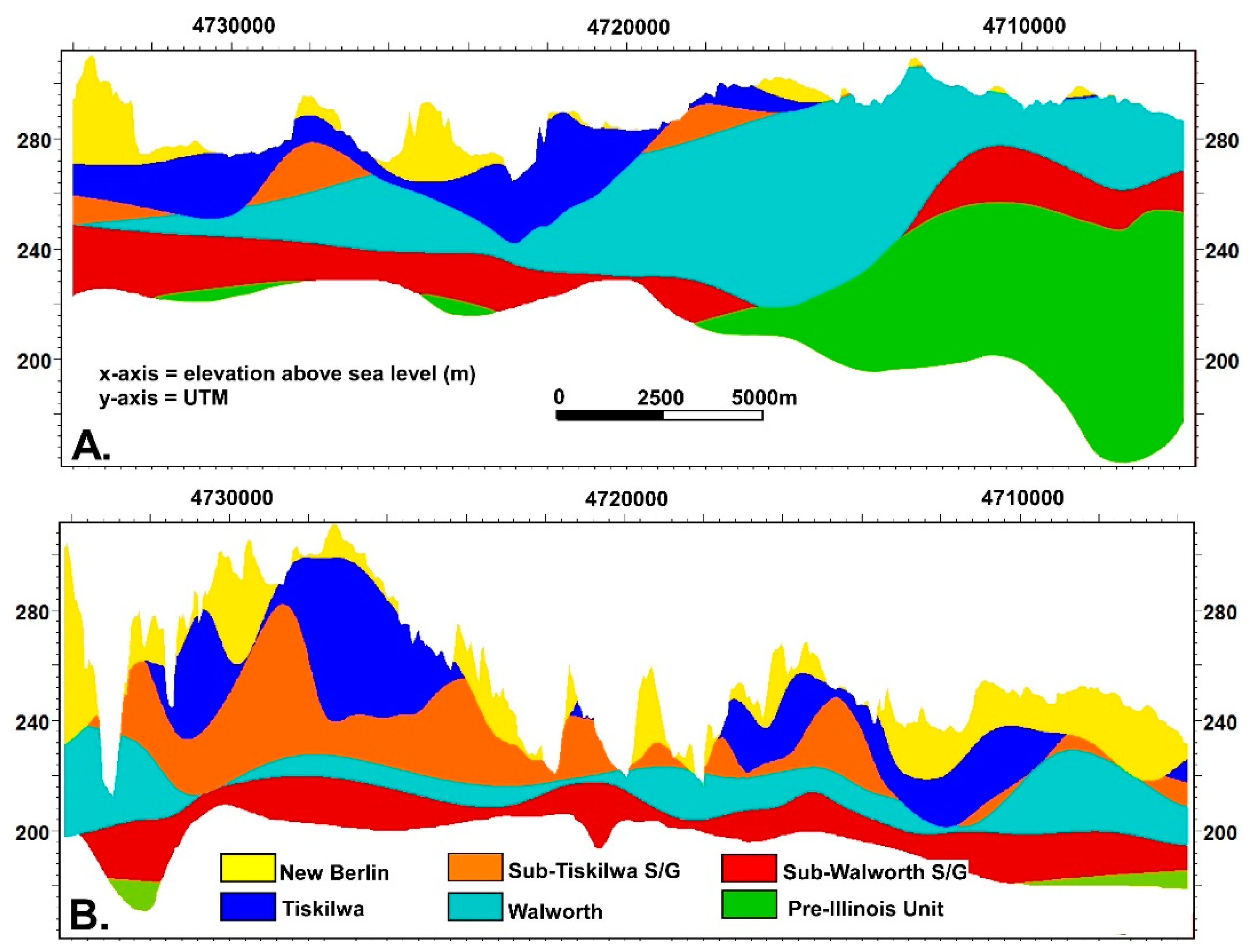
To assess the accuracy of each modeled horizon, isopach maps were generated using a standard mapping module in Petrel. For example, the surface elevation of the Sub-Tiskilwa Sand/Gravel was subtracted from the surface elevation of the Tiskilwa Formation, which generated an isopach map of the Tiskilwa Formation. This process was repeated to make isopach maps of each lithostratigraphic unit. Furthermore, model feasibility was assessed by using an interactive cross-section module in Petrel, which allows rapid 2D views of the extent, distribution, thickness, and contact relationships between the units along vertical profiles (Figure 7).

6. Results

The USGS 30-m land surface DEM was used as topographic control and as the upper boundary of the surficial New Berlin Member. Because the scope of this project was aimed at mapping largely aquifer units, surficial sand and gravel deposits (often outwash) were lumped with the New Berlin member, which is composed of sandy diamicton and sand and gravel facies. For the remaining five lithostratigraphic units, point data came solely from stratigraphic picks because those units are completely in the subsurface. To control the thickness of the Sub-Walworth Sand/Gravel, synthetic stratigraphic picks for a sixth unit (Pre-Illinois Unit) were added in bedrock valleys. The Pre-Illinois Unit was modeled to minimize potentially overthickened areas of Walworth Sand/Gravel, where borehole control is rare or absent. The distribution of the Pre-Illinois Unit is mapped completely within local bedrock valleys, but lithologic variability is not addressed.

The 3D geologic model included the six Quaternary lithostratigraphic units and a bedrock horizon as the model base. The Quaternary units include in stratigraphic order from youngest to oldest: New Berlin member of the Holy Hill Formation; Tiskilwa Member; Sub-Tiskilwa Sand/Gravel; Walworth Formation; Walworth Sand/Gravel; and the Pre-Illinois unit.

Isopach maps display the modeled thickness for each unit as follows: the New Berlin Member ranged in thickness from 0 to 80 m, the Tiskilwa Formation ranged in thickness from 0 to 80 m, the Sub-Tiskilwa Sand/Gravel ranged in thickness from 0 to 47 m, the Walworth Formation ranged in thickness from 0 to 72 m, and the Sub-Walworth Sand/Gravel ranged in thickness from 0 to 45 m. The Pre-Illinois unit is only found in bedrock valleys where it can reach a modeled maximum thickness of 94 m. However, the lithology of the Pre-Illinois Unit is unknown. Depth to bedrock ranges from a few meters to more than 160 m below ground surface.

7. Discussion

Although Petrel has rarely been used to model sediments [7,8], in this case, it was used effectively to model a complex assemblage of Quaternary deposits in Walworth County, WI. The modeled distribution and thicknesses of the units are consistent with regional interpretations of the geologic and hydrostratigraphic frameworks [13,16,17].

The New Berlin Member is typically a sandy loam diamicton that occurs as a relatively thin, semi-permeable layer (3 m thick) atop the Tiskilwa Formation. In this study, the New Berlin member included surficial sand and gravel outwash as a means to map the uppermost aquifers. An isopach map of the New Berlin Member (Figure 8) shows some relatively thick deposits (~40 m) located in the east-central portion of the map were the bedrock is high and where sand and gravel is mapped at land surface [15]. These are areas where the New Berlin till facies is likely thin or absent, and the bulk of the unit is comprised by surficial sand and gravel deposits. Localized areas in the south-central portion of study area indicate thicknesses potentially thicker than 40 m, which is correlative with the locations of end moraines (Darien, Elkhorn, and Genoa Moraines) [13], which are associated with the Delevan Sublobe of the Lake Michigan Lobe at the time of deposition of the New Berlin Member. The top surface of the New Berlin Member was generated from point data derived from a 30 m DEM and the distribution of the surficial geologic map, and thus it has seemingly the highest spatial accuracy of the modeled units.

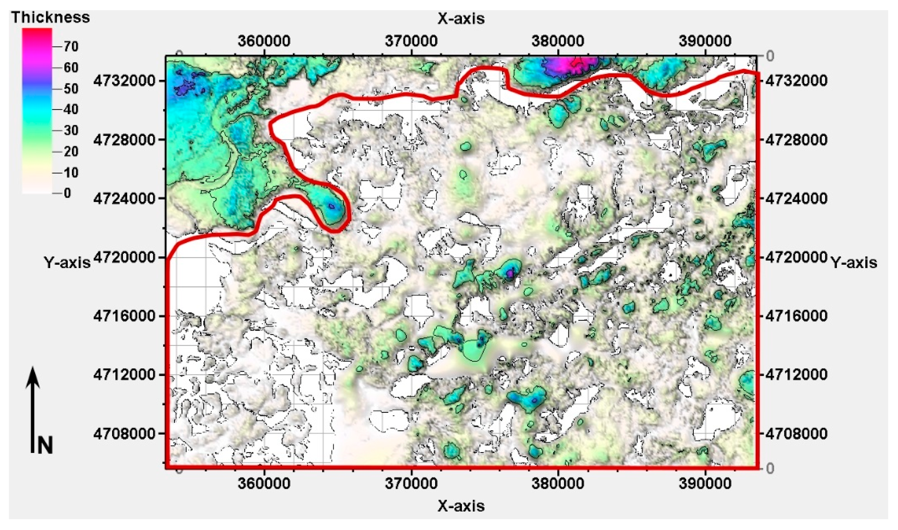
The Tiskilwa Formation was deposited by the earliest and most extensive Wisconsinan glacial advance in the area. From previous studies, a typical thickness for the Tiskilwa Formation in Walworth County is poorly known, but it is often found in the subsurface in a belt roughly 11 to 18 km wide extending from the Illinois-Wisconsin state line northward past the extent of this study area. It likely forms the core of the Elkhorn Moraine, which forms much of the belt northwest of Lake Geneva [17]. The Tiskilwa Member is a regional fined-grained confining unit for underlying sand and gravel outwash (Sub-Tiskilwa Sand/Gravel). Based on well data and known regional stratigraphy, the isopach map of the Tiskilwa Formation (Figure 9) is consistent with previous regional interpretations [13,16,17]. The Tiskilwa Formation may reach thicknesses of up to 80 m in the south-central portion of the mapping area where deposits make up the northernmost reach of the Marengo Moraine, which extends northward from Illinois. There are thick deposits of Tiskilwa Member in the subsurface below the Elkhorn, Darien, and Genoa Moraines, but those moraines are associated with the New Berlin Member. However, these results support previous interpretations that the bulk of glacial sediments that make up the shallow geology are likely associated with the Tiskilwa Member, and that the New Berlin Member is often relatively thin and drapes across older sediments [13]. Member. The Tiskilwa Member is absent in the southwest corner of the county, which is beyond the extent of the respective ice advance. The unit is interpreted as being composed mostly of subglacial till that was deposited at the base of the Lake Michigan Lobe as it advanced southwestward across Walworth County [13].

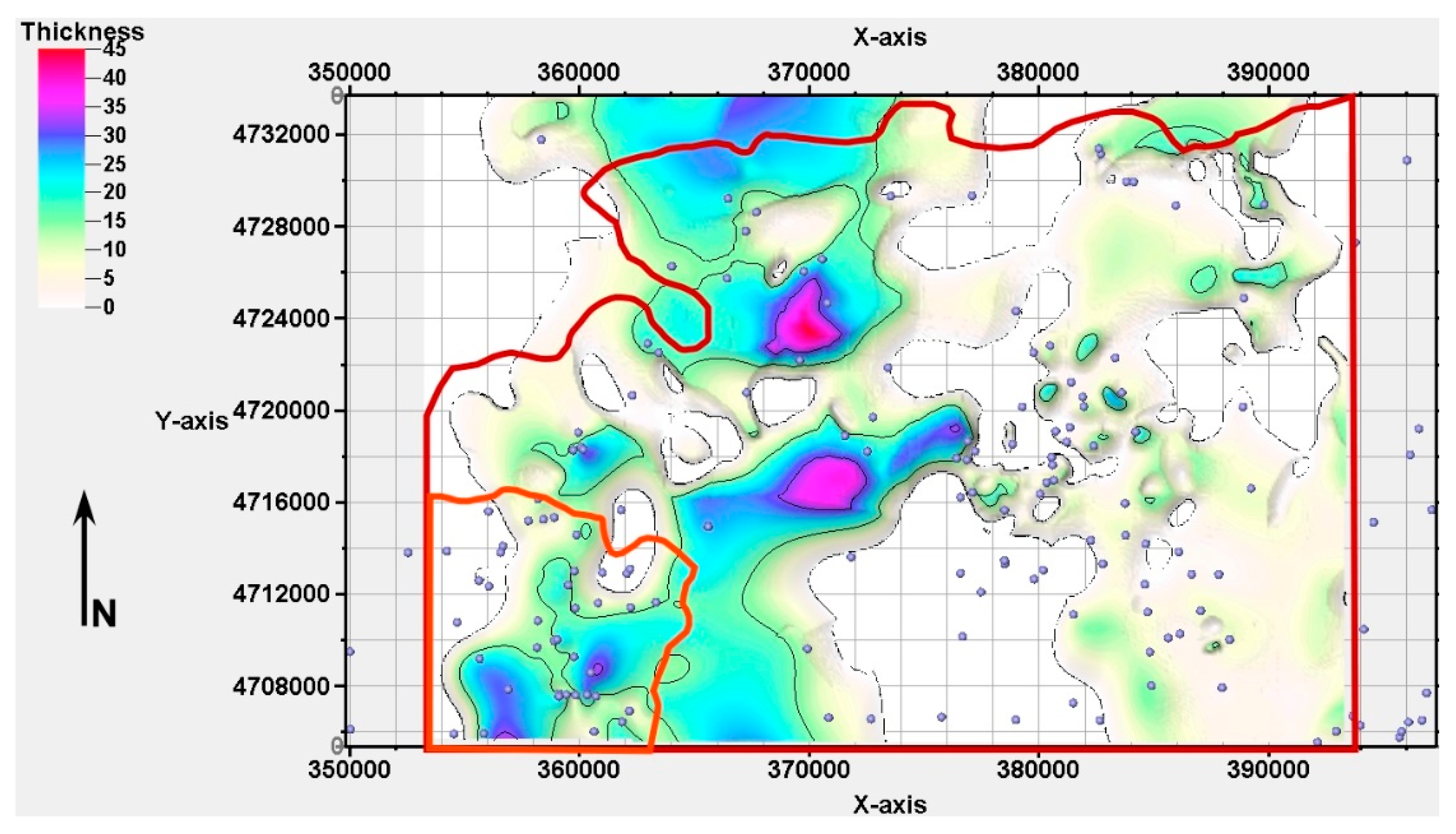
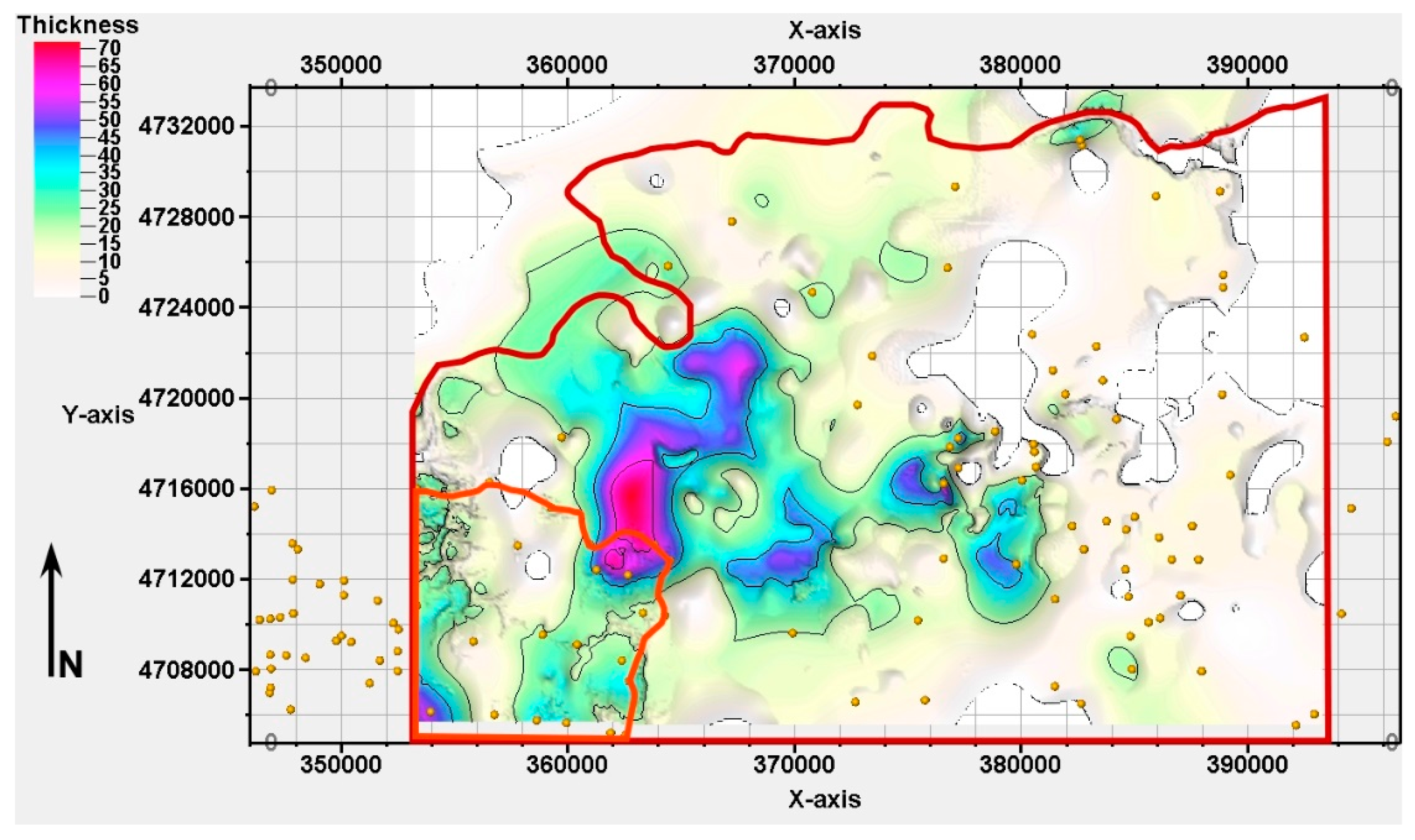
The Sub-Tiskilwa Sand/Gravel unit is equivalent to the Ashmore tongue of the Henry Formation in Illinois. There is no Wisconsin equivalent, but in Illinois, its distribution is discontinuous and it can be as thick as 30 m in southeastern McHenry County, which is adjacent to the south [18,19]. Carlock [8] reported a maximum thickness of 40 m for the Ashmore tongue in north-central McHenry County. In Walworth County, the Sub-Tiskilwa Sand/Gravel occurs as discontinuous lenses (Figure 10). The maximum thickness mapped was 47 m, which occurs in local bedrock valleys. These would be the thickest known deposits of Ashmore tongue-equivalent in the area. The north–south trending arc of greater thickness located at the center of the mapping area is consistent with trends in spatial thickness of the Tiskilwa Member and may be associated with the former terminal ice margin of that Wisconsinan advance.

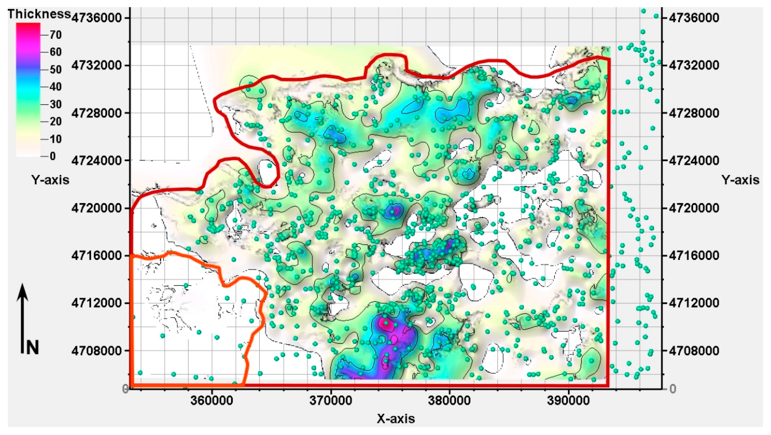
The Walworth Formation was mapped as a single unit, although it likely includes three stratigraphic members. In Wisconsin, the Walworth Formation ranges in thickness from only a few meters atop bedrock highs to approximately 80 m in Rock County, Wisconsin [17], which is adjacent to Walworth County to the west. In Walworth County, it may be mostly composed of the Fox Hollow Member [16]. The thickest deposits mapped in this study are located in the midwestern and southwestern portions of the Walworth County, where they are modeled to be up to 72 m thick (Figure 11). These sediments are interpreted as being subglacial till deposits and may likely represent a buried moraine or an area of increased subglacial deposition during the ice advance or retreat [22]. Similar to the Tiskilwa Member, the Walworth is likely a regionally extensive confining unit to underlying sand and gravel deposits. There are occasional sand and gravel lenses, or glaciolacustrine sediments, within and between till members of the Walworth Formation, but none of them were mappable or resolvable given the scope of this project.

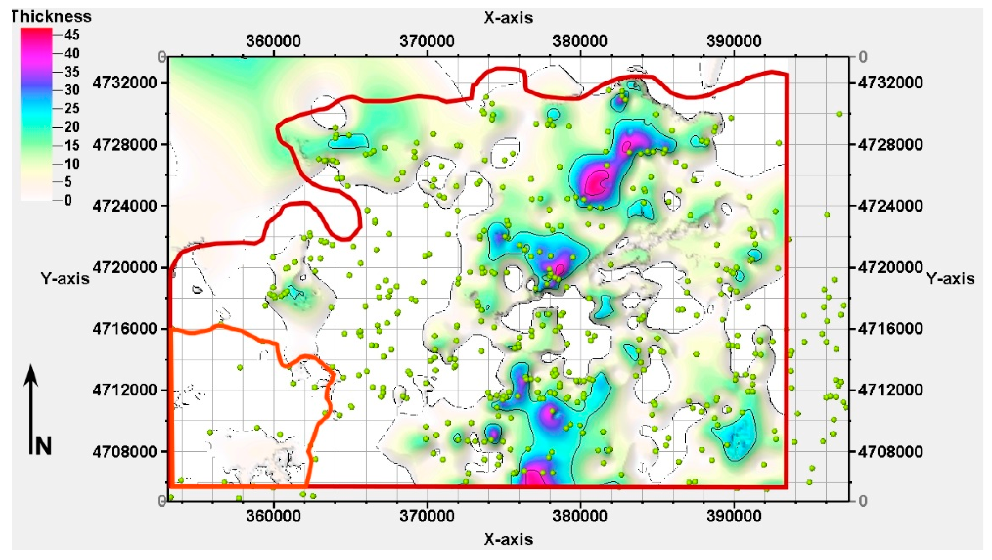
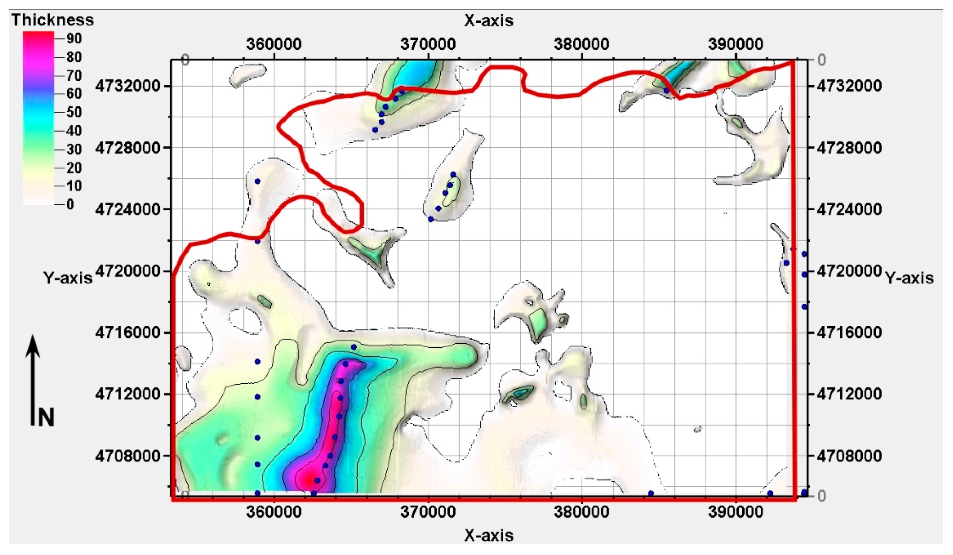
The Sub-Walworth Sand/Gravel is likely part of the unnamed sand and gravel deposits that underlie the Walworth Formation undivided [24]. It occurs as discontinuous sand and gravel lenses throughout the mapping area, but it is likely often physically and hydrologically in contact with the bedrock [16]. Although spatially variable, the unit reaches a maximum thickness of 45 m in the northwest, west-central, and southwest portions of the study area (Figure 12) where local bedrock valleys are present. Deposits of the Sub-Walworth Sand/Gravel are interpreted as outwash deposits associated with the advance of Illinois Episode glaciers, but little else is known about their sedimentology or genesis. Lastly, it may likely contribute as an aquifer resource through pumping from shallow bedrock wells.

The Pre-Illinois unit was generated entirely from synthetic boreholes for the sole purpose of controlling the Sub-Walworth Sand/Gravel thickness to reasonable values. Because the geology of the deep bedrock valleys is so poorly known, synthetic data were used to minimize overestimates of the Sub-Walworth Sand/Gravel deposits (Figure 13). These data were introduced along the linear transects of the deepest parts of bedrock valley. Consequently, the sedimentology and hydrogeologic properties of the Pre-Illinois unit in the bedrock valleys are speculative and not considered in this study.

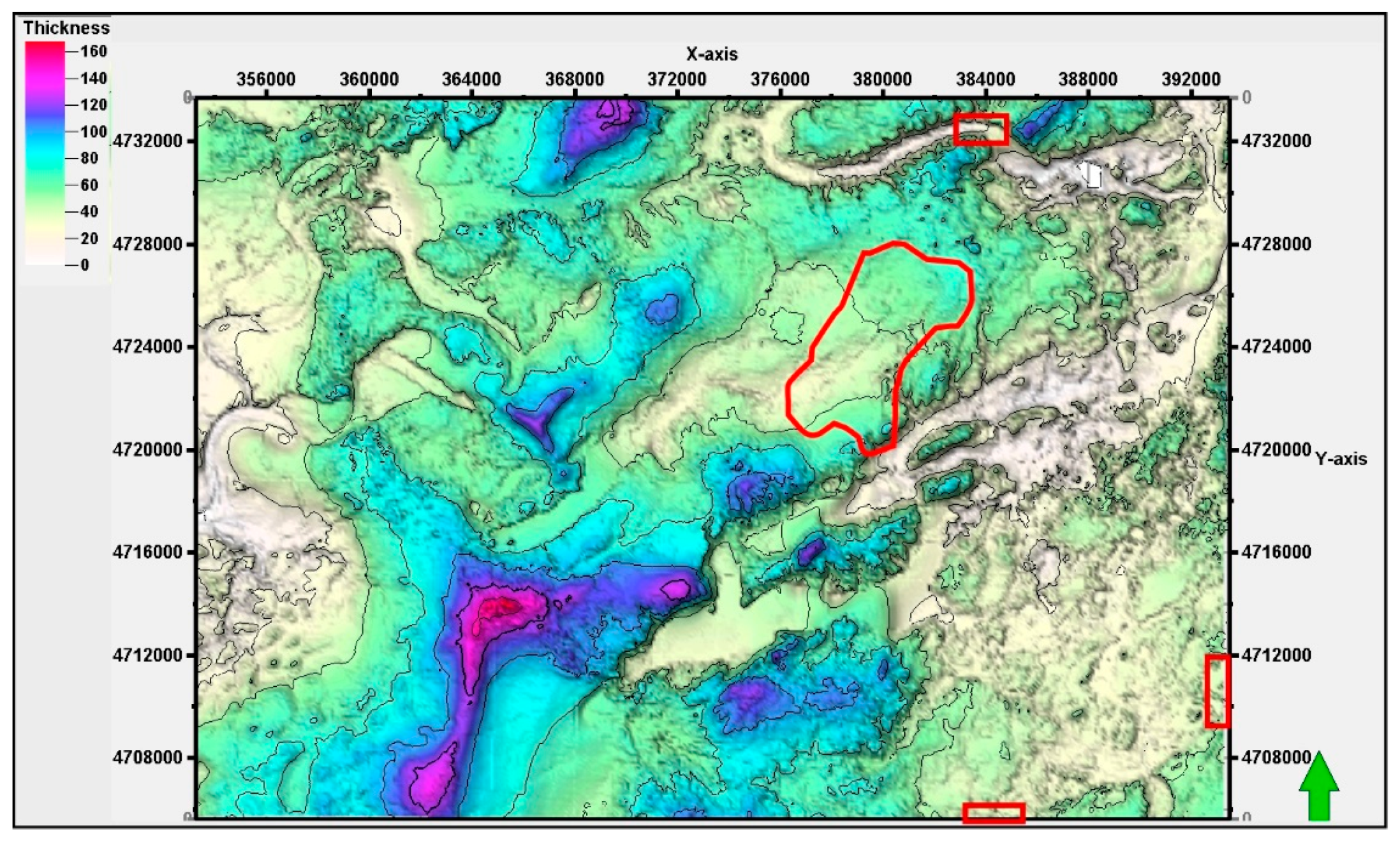
Lastly, the unpublished bedrock elevation surface provided by the WGNHS was used as the lower bounding surface of the model. It is a generalized compilation of regional bedrock surface data in southeast Wisconsin (personal communication). The bedrock surface and apparent uncertainties are consistent with more regional bedrock maps, so this lower bounding surface was reasonably correlative with water-well records (typically within a few meters). Because this study focused on Quaternary deposits, the lithologies of multiple bedrock surface units (Silurian and Cambrian-Ordovician) were not considered, but may play an important role in understanding the morphology of the bedrock surface.

8. Hydrogeologic Implications

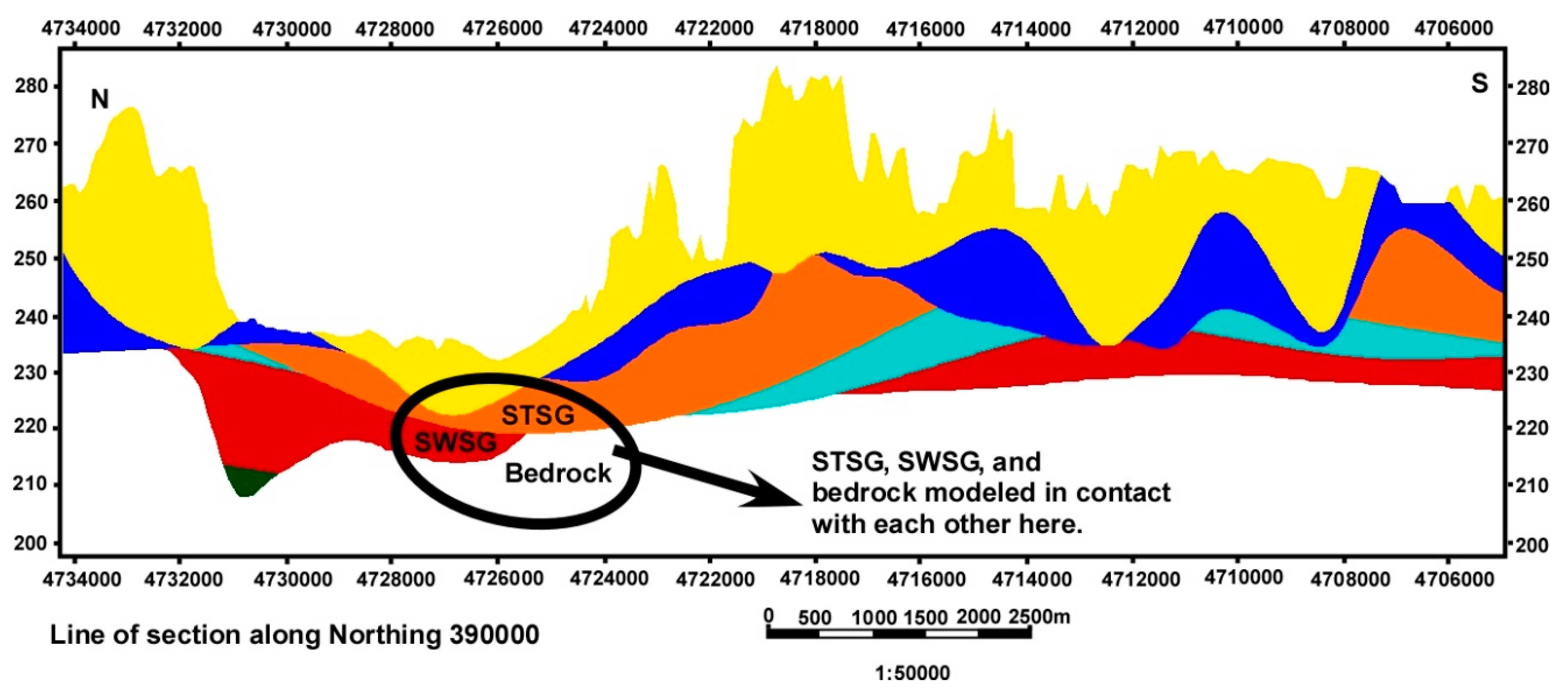
Our study was focused exclusively on delineating mappable units in the Quaternary deposits. Thus, the higher-resolution 3D mapping conducted in this study can help with integrating the Quaternary deposits in more detail for future groundwater modeling studies of the glacial deposits [16]. In this study, five units were mapped in the glacial deposits, three of which were mapped as aquifers: New Berlin, Sub-Tiskilwa Sand/Gravel (STSG), and the Sub-Walworth Sand/Gravel (SWSG). The Tiskilwa Member and the Walworth Formation are considered to be the intervening confining units. In the north and south central portions and southeastern portions of the mapping area, the Sub-Tiskilwa Sand/Gravel (STSG) and the Sub-Walworth Sand/Gravel (SWSG) were mapped to be in direct contact with each other (Figure 14). Thus, these areas may be places where the STSG, SWSG, and bedrock are all hydraulically connected and may be sensitive areas when considering bedrock aquifer recharge and contamination potential.

The southwestern portion of the county may be an important recharge area for both the STSG and the SWSG. The surficial geologic map indicates sand and gravel deposits (alluvial fan deposits [21] at land surface, and water well records indicate that these deposits may be relatively thick (about 20 m). The thickness of the STSG in this area ranges from 15 to 24 m in the subsurface. It is not likely that the STSG aquifer is in direct contact with the bedrock aquifer it is underlain by relatively continuous deposits of the Walworth Formation (5 to 72 m). However, because these Quaternary deposits fill the Troy Bedrock Valley and the fine-grained Maquoketa shale (a regional aquifer confining unit) is eroded in the valley, this location may be an important recharge area for the regional bedrock aquifer.

In the northeastern and southeastern portions of the study area, the bedrock is generally shallow at depths of 10 to 80 m. The Tiskilwa Member and Walworth Formation often pinch out against these bedrock highs. In these areas, it is unclear whether these confining units were eroded or simply not deposited. In any case, these may be additional locations where the STSG, SWSG and bedrock are hydraulically connected (Figure 15).

The most recent groundwater study in Walworth County was completed by Gotkowitz and Carter [16]. Their study found that the regional hydrogeologic flow regime in Walworth County is highly affected by the variability in the type and thickness of glacial sediments of the Wisconsin Episode of glaciation. In that study, the regional stratigraphy of the Quaternary deposits were discussed, but for groundwater-flow modeling purposes, those deposits were generalized into three hydrostratigraphic units. Thus, variability within and between sand and gravel units was addressed in the model, but it was likely not optimal. That study effectively concluded that varying pumping scenarios might help minimize pumping effects on groundwater discharge to a local lake. Many of those pumping wells are finished in shallow sand and gravel aquifers, where improved understanding of aquifer distribution and thickness would be valuable. Thus, the results of our study can help address uncertainty in future modeling studies in Walworth County and also address the impacts of better understanding of shallow aquifer system variability in general.