Evaluation of the Snow Thermal Model (SNTHERM) through Continuous in situ Observations of Snow’s Physical Properties at the CREST-SAFE Field Experiment

Abstract

Snowpack properties like temperature or density are the result of a complex energy and mass balance process in the snowpack that varies temporally and spatially. The Snow Thermal Model (SNTHERM) is a 1-dimensional model, energy and mass balance-driven, that simulates these properties. This article analyzes the simulated snowpack properties using SNTHERM forced with two datasets, namely measured meteorological data at the Cooperative Remote Sensing Science and Technology-Snow Analysis and Field Experiment (CREST-SAFE) site and the National Land Data Assimilation System (NLDAS). The study area is located on the premises of Caribou Municipal Airport at Caribou (ME, USA). The model evaluation is based on properties such as snow depth, snow water equivalent, and snow density, in addition to a layer-by-layer comparison of snowpack properties. The simulations were assessed with precise in situ observations collected at the CREST-SAFE site. The outputs of the SNTHERM model showed very good agreement with observed data in properties like snow depth, snow water equivalent, and average temperature. Conversely, the model was not very efficient when simulating properties like temperature and grain size in different layers of the snowpack.

1. Introduction

Information on snowpack properties is of great interest to the hydrologists’ community. Applications like water availability, reservoirs managing, flood forecasting, and assessing climate change impacts are just a few examples in which these data play a critical role [1,2,3]. For this reason, many efforts have been devoted to making this information available [4,5,6].

The conventional source of acquiring snow characteristic information is reports from a network of ground-based meteorological stations in which daily observations are performed [7,8]. However, most of Earth’s snow is located in remote and inaccessible areas, where populations are sparse or nonexistent and extreme conditions limit the continuous characterization of the snow conditions.

Snow Physical Models (SPMs) and satellite remote sensing have been used for estimation of the snowpack properties for several decades [9,10,11,12]. A combination or synergistic approach can provide higher spatial and temporal resolutions than conventional, ground-based methods [13,14,15,16,17]. However, one question that is still unresolved is: What level of accuracy can be reached using snow physical models with several input sources?

SPMs can produce snowpack properties [18,19], but they depend on externally supplied datasets of precipitation, radiation, temperature, winds, relative humidity, and barometric pressure to simulate land surface states, and errors in any of these inputs can impact the simulation results [20]. The required ground observations to run the models can only be collected at National Weather Service Offices (NWSO) sites or research sites, and both are very sparse and scarce around the United States. As a result, spatially and temporally continuous simulation of snowpack properties is very challenging when using only ground-based measurements. That is where Data Assimilation Systems (DAS), which are a combination of remote sensing products (airborne and satellite observations), ground-based measurements and estimations based on interpolation methods and stochastic approximations, can prove a useful alternative that provides spatially and temporally-continuous meteorological data [21,22].

The accuracy of the simulated snowpack properties is determined by the accuracy of the models and the accuracy of the input data. In this paper, two frameworks to simulate snowpack properties are evaluated. The capabilities of the Snow Thermal Model (SNTHERM), an energy and mass balance-driven snowpack model [12], was evaluated using two different sets of meteorological data: observed data at the Cooperative Remote Sensing Science and Technology-Snow Analysis and Field Experiment (CREST-SAFE) site [23] and assimilated data from National Land Data Assimilation System (NLDAS) [21]. The results were compared with in situ observed snowpack properties at the CREST-SAFE site.

Multiple studies have demonstrated that SNTHERM successfully simulates the snowpack properties at diverse locations and under varying conditions, both as a standalone model and coupled with other models [24,25,26]. However, the scarcity of detailed and long term and continuous (from on-set to melt-out) observed data limited the validation of the studies. On the other hand, the path forward for snowpack properties retrievals is the synergy among different existing snow products and models [17,27,28]. Thus, long term and exhaustive validation of the model is still needed.

However, the performance of SNTHERM has been evaluated several times for different sites, though these assessments have only included the following parameters: snow depth, snow water equivalent, density, and average temperature [23,24]. However, the task of assessing the variation of the snowpack properties within the snowpack layers has never been undertaken before.

This study represents the first attempt to assess the efficiency of SNTHERM using meteorological variables from ground-based observations and data assimilation systems, based on the evaluation of snowpack properties (e.g., snow depth, snow water equivalent, and snow temperature) and a layer by layer comparison.

The performance of the SNTRHERM model is assessed with in situ observations at CREST-SAFE as well as NLDAS data as input variables. This assessment is significant because in situ data, if obtained adequately, is a robust source of meteorological parameters. However, this information is rarely available and spatially distributed data such as NLDAS could be incorporated to complement the input required for snowpack properties simulation. The CREST-SAFE site was designed and installed with several objectives, e.g. the testing, validation, and improvements of SPMs and Radiative Transfer Models (RTM) [23]. On the other hand, for satellite product validation, spatially distributed data is required.

2. Study Area

The CREST-SAFE site [23] is located in Caribou, ME, north of the Northeastern region in the United States. Caribou has a humid continental climate, with long, snowy winters, and warm, humid summers. The monthly mean temperature ranges from −12.5 °C in January to 18.7 °C in July. There are approximately 44 nights per winter that drop to −18 °C or below. Measurable snowfalls can occur as early as mid-October and as late as the last week of April, but significant snowfalls do not usually occur until mid-November, and are usually finished by early April. In general, Caribou offers the ideal conditions for maritime snow studies; the normal seasonal snowfall for Caribou is approximately 2.90 m with a record snowfall of 5.02 m set in the winter of 2007–2008. The seasonal snow accumulation reaches its maximum by the end of February beginning of March and amounts usually to 50–60 cm.

The CREST-SAFE station is located next to the Regional National Weather Service office on the premises of the Caribou Municipal Airport at Caribou, ME, USA (Figure 1). The quality-controlled location and with relatively flat topography offers the optimum environment for model validation. As for land cover/use, the site is just outside the urbanized area of Caribou, and it is covered by grass with some canopy present more than 10 m apart of the site where measurements are recorded. The top soil layer (50 cm) is a mixture of mainly clay with some encrusted rock organic matter.

Figure 1. Cooperative Remote Sensing Science and Technology-Snow Analysis and Field Experiment (CREST-SAFE) site location. Adapted from Lakhankar 2013 [23].

Figure 1. Cooperative Remote Sensing Science and Technology-Snow Analysis and Field Experiment (CREST-SAFE) site location. Adapted from Lakhankar 2013 [23].

3. The Snow Thermal Model (SNTHERM)

The Snow Thermal Model (SNTHERM) is a freely available, Fortran-written, one-dimensional snowpack model that was first released on 1989. It has been enhanced since then several times to include improvements and upgrades to its algorithms [12]. It is energy and mass balance-driven and it can be considered one the most robust models available nowadays. It has been used in several validation studies like spectral signature of the snowpack [29], snow melting processes in Greenland ice sheet [30], energy balance at continental scale, discrete point scale, and under the canopy [31,32]. A simplified version of the model is currently operational for snow mapping and forecasting in the United States [18,33,34] and Bosnia [35]. SNTHERM was based initially on the mass and energy-balance snow model of Anderson 1976 [36]. However, it also incorporates several other theories for snowpack properties, including dynamic snowfall density as defined by Anderson in 1976, which is based on data collected by LaChapelle 1969 [36]. Anderson used an empirical equation where New Snow Density (bifall) is a function of the wet bulb temperature (Tw) in Kelvin degrees.

The vertical water movement is based on the work done by Colbeck [37], in which the effective saturation of snow (se) is a function of the current saturation level (s) and the irreducible water saturation (ssisnow). Snowpack layer densification is calculated based on three main processes, namely destructive metamorphism or overburden compaction, constructive metamorphism or vapor movement and grain size change, and melt metamorphism or the gravitational water movement inside the snowpack [36,38,39,40]. The first two are merged into an overall compaction rate (CR) and the third metamorphism type is calculated based on the water balance. Destructive metamorphism is calculated as a function of snow viscosity (eta0) [38,39]. Constructive metamorphism is a function of temperature and it is a process that has a faster rate when new snow density is greater than the density limit (dmlimit) constant [36].

As described in the Special Report 91-16 of the United States Army Corps of Engineers [12] and reported by Melloh 1999 [41], the SNTHERM numerical solution is obtained using a variable grid of snow layers, each layer is governed by heat and mass balance equations. The model uses a control volume numerical procedure [42] for spatial discretization that allows compaction of the snow cover. A Crank-Nicholson central difference scheme is used to solve the partial differential equations in the time domain.

3.1. Datasets

This study focused in the snowpack properties simulation for three complete winters (from accumulation period to total ablation) for which ground-based data was available. Specifically, the observed weather conditions for the 2010–2013 winters were input to SNTHERM. The two meteorological data sources utilized are CREST-SAFE and NLDAS.

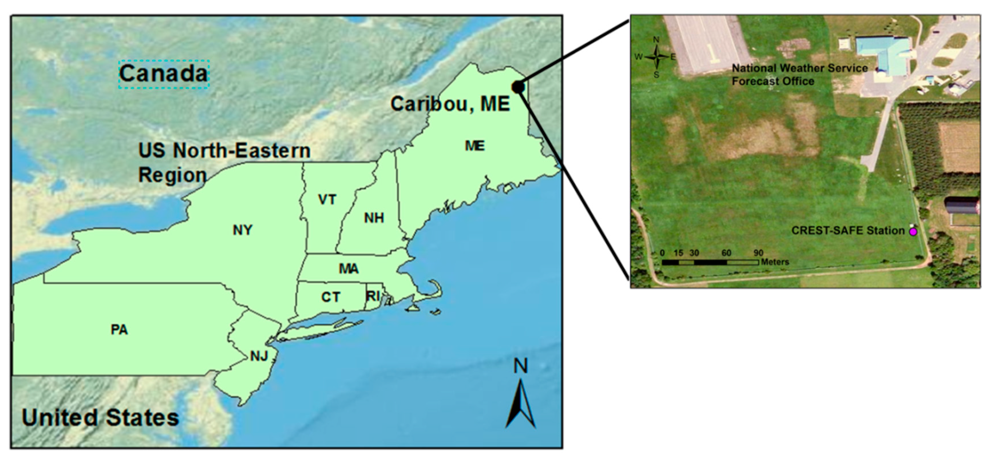
3.2. CREST-Snow Analysis and Field Experiment (CREST-SAFE)

The CREST-SAFE experiment is a long-term field campaign where meteorological variables and snowpack properties are measured. The measured meteorological variables are: temperature, solar radiation, relative humidity, and wind speed and direction. The studied snowpack properties are depth, snow water equivalent (SWE), temperature of snow layers, grain size, density, and snow microwave emission at 89, 37 and 19 GHz. A detailed characterization of the instruments and site is described in [23,43] and the archive and real-time data are available for the public and scientific community at the experiment website [44]. The only meteorological parameter that it is not measured in the CREST-SAFE site, and is needed for simulation, is precipitation. Consequently, for simulation purposes, it was obtained from the National Weather Service (NWS) Station named KCAR [8], located near the CREST-SAFE site, at the Caribou Municipal Airport, Caribou, ME. The precipitation classification was performed by the model, based on its built-in algorithm [12]. CREST-SAFE station provides all its data in an hourly time step from the installed instruments on its automated routine [23] and NWS provides the precipitation in 15 minutes time steps, which was resized to hourly.

3.3. The National Land Data Assimilation System (NLDAS)

In order to improve snow characteristic prediction by dynamical models, reliable weather forcing data is required; in this study, the CREST-SAFE’s weather observations are complemented with the NLDAS Forcing Data L4 Hourly 0.125° × 0.125°. This dataset is a national product that merges and downscales remote sensing and ground-based measurements of meteorological data for the continental United States [20]. Comparisons between NLDAS meteorological data and the locally-observed forcing shows a fair to good agreement between the datasets [20,45,46].

It is clear that NLDAS is a coarse resolution dataset that will never surpass the results that can be obtained with robust information such as CREST-SAFE observations. However, it does show potential to be used as a meteorological input in physical models that are able to effectively and efficiently simulate snowpack properties.

SNTHERM capacity is limited to the input data accuracy and therefore the use of data assimilations systems should be restricted to places in which in situ observations are not available. NLDAS dataset contains all the necessary inputs needed for SNTHERM simulations in an hourly time step. Table 1 shows the meteorological variables needed to run the SNTHERM model. Several publications compared and attempted to validate the NLDAS dataset in several regions of the continental United States [20,22,45,47,48,49]. Some of the previously published articles focused in the meteorological data validation. Conversely, others have focused on the effects of using this meteorological data for modeling purposes. In general, NLDAS has shown potential as a weather forcing data set. 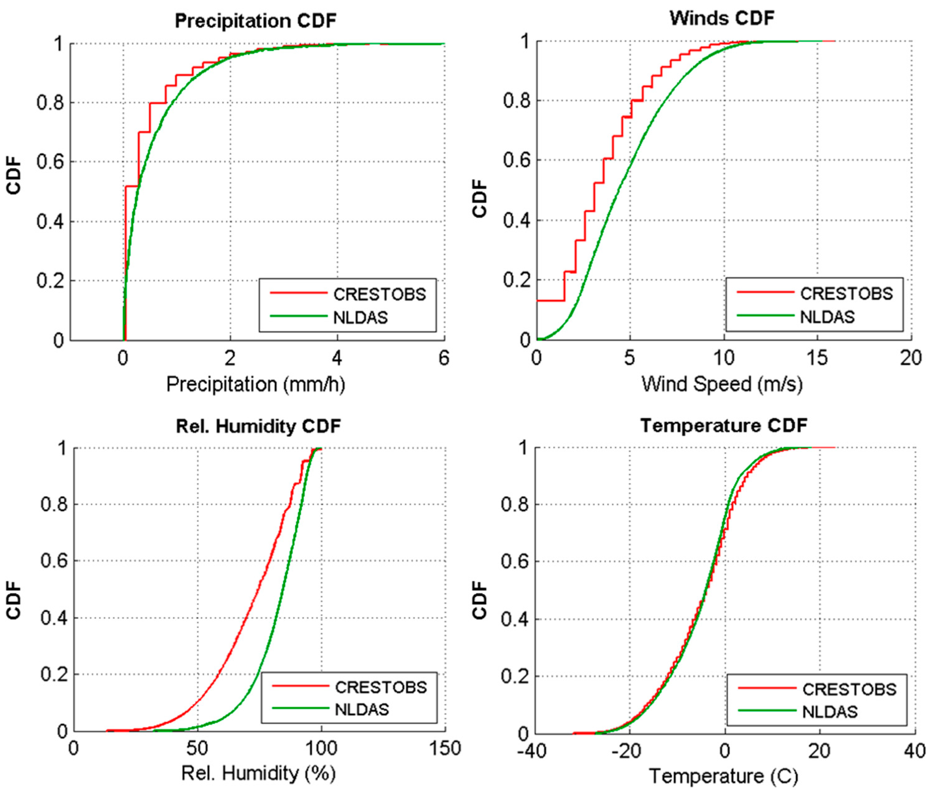Figure 2 shows a comparison for the observed meteorological variables at CREST-SAFE stations (CRESTOBS) and the co-located pixel of NLDAS dataset for the different meteorological input variables.

Table 1. SNTHERM model inputs list and sources. Source 01 is CREST-SAFE observed meteorological data, Source 02 is NLDAS data, Source 03 is a national weather service station, and Source 04 is the National Climatic Data Center (NCDC) FM Report.

Snow Thermal Model Inputs
Name	Variable Symbol	Units	Note	Used Source
Air temperature	T	°K	-	01/02
Wind Speed	WS	m/s	-	01/02
Relative Humidity	RH	%	-	01/02
Precipitation water equivalent	PR	m/s	-	02/03
Precipitation type	Pty	-	Optional	Not used
Incoming Solar	KD	W/m2	-	01/02
Down welling long wave	LD	W/m2	-	01/02
Cloud Cover (at 3 layers)	CC	%	Optional	04
Cloud Type (at 3 layers)	CT	-	Optional	04

Table 1. SNTHERM model inputs list and sources. Source 01 is CREST-SAFE observed meteorological data, Source 02 is NLDAS data, Source 03 is a national weather service station, and Source 04 is the National Climatic Data Center (NCDC) FM Report.

Snow Thermal Model Inputs
Name	Variable Symbol	Units	Note	Used Source
Air temperature	T	°K	-	01/02
Wind Speed	WS	m/s	-	01/02
Relative Humidity	RH	%	-	01/02
Precipitation water equivalent	PR	m/s	-	02/03
Precipitation type	Pty	-	Optional	Not used
Incoming Solar	KD	W/m2	-	01/02
Down welling long wave	LD	W/m2	-	01/02
Cloud Cover (at 3 layers)	CC	%	Optional	04
Cloud Type (at 3 layers)	CT	-	Optional	04

Figure 2. Meteorological data cumulative distribution function (CDF) of observed meteorological data (CRESTOBS) and assimilated meteorological data from the National Land Data Assimilation System (NLDAS). Variables in figures: precipitation (upper left); Winds (upper right); relative humidity (lower left); and temperature (lower right).

Figure 2. Meteorological data cumulative distribution function (CDF) of observed meteorological data (CRESTOBS) and assimilated meteorological data from the National Land Data Assimilation System (NLDAS). Variables in figures: precipitation (upper left); Winds (upper right); relative humidity (lower left); and temperature (lower right).

Considering CREST-SAFE observations as ground truth, there is overestimation of wind speed and relative humidity in the NLDAS dataset, shown by the shift towards the right in both cumulative distribution function (CDF) curves when compared to the observed. On the other hand, precipitation and temperature CDFs showed good agreement. The objective of this work is not to compare or assess the meteorological data but rather the accuracy of the SNTHERM model and the effects of forcing it with the two datasets (CREST-SAFE and NLDAS). Future work will include an assessment of the effect of the biases (Figure 2) in the simulation process.

4. Methodology

In this study, the observed weather conditions for the 2010–2011, 2011–2012, and 2012–2013 winters were used as an input to the SNTHERM model. Then, the simulated snowpack properties were compared with measured snowpack properties collected in the CREST-SAFE site using automatic sensors and manual pits throughout the aforementioned winters.

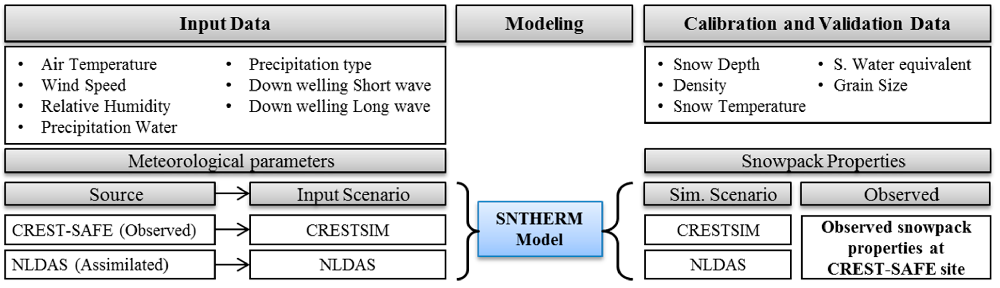
The performance of the SNTRHERM model is assessed with in situ observations at CREST-SAFE as well as NLDAS data as input variables (Figure 3). The National Land Data Assimilation System (NLDAS) [47] was used as a support method due to the current interest of investigating the strength of this weather forcing dataset for simulation purposes when ground-truth data is not available. The simulated snowpack properties (depth, grain size, density, temperature, and snow water equivalent) were compared to field observations at CREST-SAFE site. Calibration of the SNTHERM model was performed using two winters out of the three available. Validation was performed over the remaining winter. Alternating between calibration and validation period allowed obtaining a complete set of 3 winters for validation. The general framework of this methodology is shown in Figure 3.

Figure 3. Flowchart of datasets, modeling setup, and general scope of work. Meteorological data was processed from CREST-SAFE station (CRESTSIM input/simulation scenario) and NLDAS assimilation system (for NLDAS input/simulation scenario); observed snowpack properties at the CREST-SAFE site were used to calibrate and validate the model.

Figure 3. Flowchart of datasets, modeling setup, and general scope of work. Meteorological data was processed from CREST-SAFE station (CRESTSIM input/simulation scenario) and NLDAS assimilation system (for NLDAS input/simulation scenario); observed snowpack properties at the CREST-SAFE site were used to calibrate and validate the model.

To measure the efficiency of the model in both simulated scenarios (CREST-SAFE and NLDAS meteorological data), two assessments were performed. Both assessments were performed in the validation period. The validation period consists in the combination of the three validation periods for the three calibration scenarios presented on the model calibration section. The first assessment was based on snow depth, snow water equivalent, and snow density. The second assessment is a layer-by-layer comparison of snowpack properties.

Since most of the energy and mass fluxes of the snowpack occur in the bottom and top layers of the snowpack, the second assessment was based on two layers (Top and Bottom) of the snowpack and the average of the complete snowpack. The top layer is defined as the top 5 cm of the snowpack, the bottom layer is the bottom 5 cm of the snowpack, and the average is the average value of the measured parameter throughout the entire snowpack depth.

4.1. Statistical Analysis

The efficiency of the model was measured based on statistical and goodness of fit measures, namely the root square error (RMSE), the correlation coefficient (R²), and the Kling-Gupta Efficiency (KGE) index. The selected measurements are widely used throughout the scientific community and simultaneous analysis of the indexes will define how close the simulations are to the observed data. In general, the larger the RMSE values, the more significant the errors associated with the simulation. Furthermore, low R² values will indicate low ability of the model to represent the variability of the phenomena. Finally, other authors [50,51] and recent works [52,53] suggest that the KGE index is a powerful tool for quantitative assessment of hydrological and land surface models. The KGE function quantifies three important aspects: (i) the correlation between simulated and observed values; (ii) the relative variability in the simulated and observed values; and (iii) the bias error.

A correlation greater than 0.80 is generally described as strong, whereas a correlation less than 0.50 is described as weak. In this study, a good simulation is defined as having an R² greater than 0.70, an RMSE less than half the observed standard deviation (SD_obs) [54], and a statistical value from Student’s t-test lower than the critical value. The critical value for samples of 29 elements is ±2.06 and for samples over 150 elements is ±1.98. For goodness of fit index such as the KGE, the general performance is considered good for values greater than 0.75 [54].

The Equations (1)–(4) are used for the statistical analysis performed in this work, with Y_n,obs; observed variable at time step n, $\overline{Y}$_obs; average observed variable at time step n, Y_n,sim; simulated variable at time step n, $\overline{Y}$_sim; average simulated variable at time step n, N; number of observed/simulated points, RMSE is Root Mean Squared Error, R² is the correlational coefficient, t is the statistical value from Student’s t-test, SD_sim is the standard deviation of the simulated variable, CV_sim is the coefficient of variation for the simulated variable, and CV_obs is the coefficient of variation for the observed variable.

$${\text{SD}}_{\text{obs}}=\sqrt{\frac{{\displaystyle \sum _{n=1}^N{\left(Y_{n,\text{obs}}-{\overline{Y}}_{\text{obs}}\right)}^2}}{N-1}}$$

(1)

$$\text{RMSE}=\sqrt{\frac{{\displaystyle \sum _{n=1}^N{\left(Y_{n,\text{obs}}-Y_{n,\text{sim}}\right)}^2}}{N-1}}$$

(2)

$$R^2=\frac{{\left\{{\displaystyle \sum _{n=1}^N\left[\left(Y_{n,\text{obs}}-{\overline{Y}}_{\text{obs}}\right)\cdot \left(Y_{n,\text{sim}}-{\overline{Y}}_{\text{sim}}\right)\right]}\right\}}^2}{{\displaystyle \sum _{n=1}^N{\left(Y_{n,\text{obs}}-{\overline{Y}}_{\text{obs}}\right)}^2}\cdot {\displaystyle \sum _{n=1}^N{\left(Y_{n,\text{sim}}-{\overline{Y}}_{\text{sim}}\right)}^2}}$$

(3)

$$t=\frac{{\overline{Y}}_{\text{obs}}-{\overline{Y}}_{\text{sim}}}{\sqrt{\frac{{{\text{SD}}_{\text{obs}}}^2}{N}+\frac{{{\text{SD}}_{\text{sim}}}^2}{N}}}$$

(4)

$$\text{KGE}=1-\sqrt{{\left(R-1\right)}^2+{\left(\frac{{\overline{Y}}_{\text{sim}}}{{\overline{Y}}_{\text{obs}}}-1\right)}^2+{\left(\frac{{\text{CV}}_{\text{sim}}}{{\text{CV}}_{\text{obs}}}-1\right)}^2}$$

(5)

4.2. Model Calibration

A site-specific sensitivity analysis was carried out to determine the most sensitive parameters of the model that affect snow depth and snow water equivalent of the snowpack. A genetic algorithm (GA) optimization scheme [55] was used to generate combinations of parameters and minimize an objective function. The objective function was defined as the RMSE between observed and simulated snow depth.

The GA scheme produces a set of 20 random combinations of four (4) selected parameters values within the assigned range for first iteration. The model is executed for each combination and the objective function value (RMSE) is calculated for each of them. The combinations are ranked based on their objective function values. The top three (3) ranked combinations are selected for the next iteration exactly as they are, the next seven (7) are partially modified by changing 50% of the parameters (two), and the remaining ten (10) combinations are substituted by new combinations generated randomly. Approximately 1496 different combinations are generated in 88 iterations. The algorithm stops when the stopping criterion is reached. In this case, the stopping criterion was a maximum number of generated combinations, set to 1500. This optimization process has shown to be very efficient; 1500 combinations were considered sufficient to ensure stability of the solution given the value range and step change for the parameters.

The calibration period was the combination of winter 2010–2011 and winter 2012–2013. Out of the 1500 combinations of parameters generated within the GA scheme, the top 10 were further analyzed. The parameter set closest to the default values was selected as the optimum parameter combination. The same procedure was used alternating the calibration and validation period (e.g., using winters 2011–2012 and 2012–2013 for calibration and using 2010–2011 as validation period). As it was expected, all the calibrations setup offered very similar results for optimum parameter set.

The parameters in the first column of Table 2 were selected from the manual sensitivity analysis for calibration. The third column shows the range used for calibration and the fourth column shows the change step for the parameter within the calibration setup. The fifth column shows the default value of the parameter and the sixth column shows the value used in the simulations. The validation period selected to show results was winter 2011–2012.

Table 2. Model parameters description, calibration range, change step for calibration, and parameter value after calibration.

Parameter	Name	Calibration Range	Change Step	Default	Used	Units
Ssisnow	Irreducible water content for Snow	0.01–0.10	0.001	0.04	0.017	-
Bifall	Density of new snow	50–150	1	80	73	kg/m3
dmlimit	Density limit for compaction of snow	50–200	1	100	96	kg/m3
eta0	Viscosity coefficient for overburden compaction	4 × 105–4 × 106	1 × 104	9 × 105	6.9 × 105	kg·s/m2

Table 2. Model parameters description, calibration range, change step for calibration, and parameter value after calibration.

Parameter	Name	Calibration Range	Change Step	Default	Used	Units
Ssisnow	Irreducible water content for Snow	0.01–0.10	0.001	0.04	0.017	-
Bifall	Density of new snow	50–150	1	80	73	kg/m3
dmlimit	Density limit for compaction of snow	50–200	1	100	96	kg/m3
eta0	Viscosity coefficient for overburden compaction	4 × 105–4 × 106	1 × 104	9 × 105	6.9 × 105	kg·s/m2

A detailed explanation of the parameters can be found in Jordan 1991 [12]. The calibration range, as well as the final decision of values used, was based on previous work done by Anderson 1976, Mellor and Kojima 1967, Kattelmann 1986, and Jordan 1991 [12,36,38,39,40]. Irreducible water content for snow (ssisnow) is the minimum amount of water that can have a layer of snow, controlling evaporation and sublimation in the snowpack. Density of new snow (bifall) is the assumed density for the snow precipitation. Density limit for compaction of snow (dmlimit) is the upper limit on destructive metamorphism compaction. Finally, the viscosity coefficient (eta0) controls the compaction rate of snowpack due to overburden.

5. Results and Discussions

5.1. Snow Depth and Snow Water Equivalent

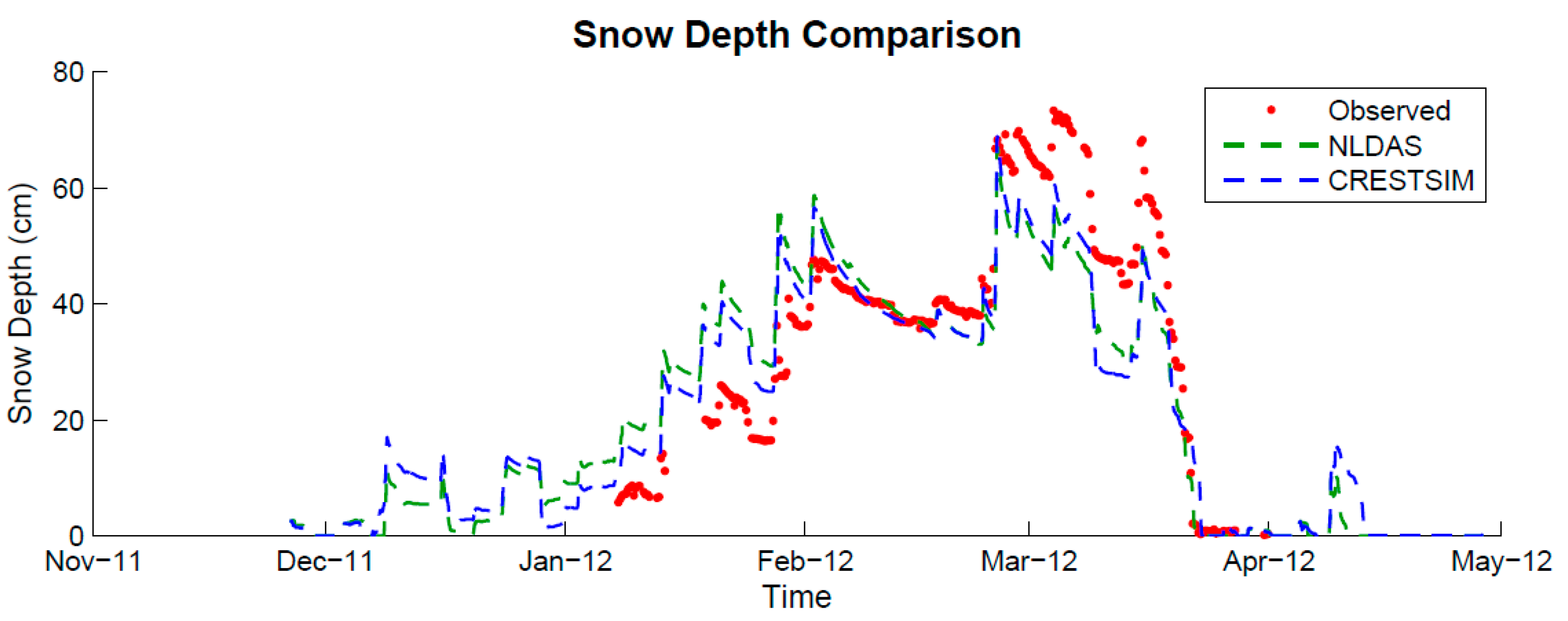
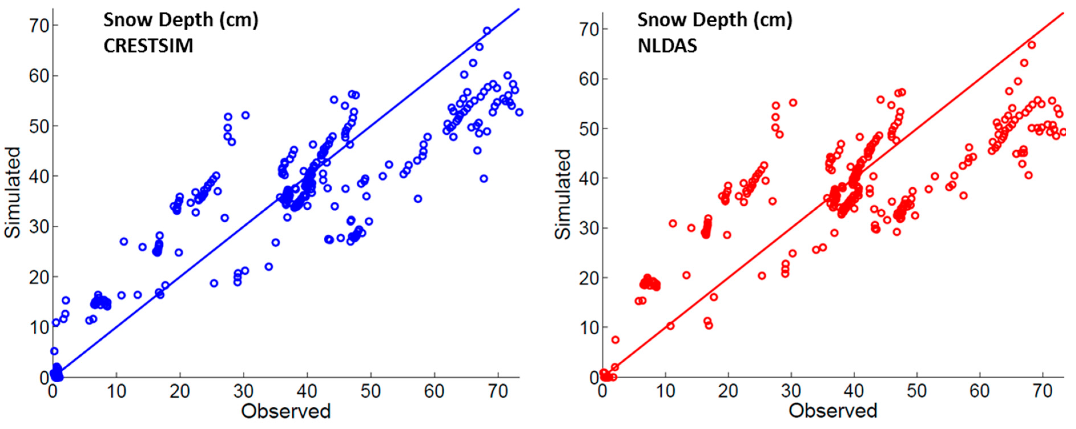
The model successfully predicted timing and magnitude of variations in snow depth (Figure 4), including the total melt out time. Overall, CRESTSIM was more accurate in simulating snow depth (Figure 5). This performance shows how reliable forcing data produce better land surface modeling results. Figure 5 also depicts that CRESTSIM scenario exhibited a slight overestimation in the accumulation period (before March) and underestimation in the ablation period (after March). It is suspected that the model parametrization of the snow thermal properties caused this divergence in the simulations. Using 2012 as a study case, the analysis shows the higher the concurrence between simulated snowpack temperature and observed data, the higher the agreement in the simulations. However, in seasonal terms, as shown in the statistics on Table 3, there is very good agreement between the observed and simulated data when using CREST-SAFE.

For CRESTSIM, its high R² (≥0.70) and KGE (≥0.75) values indicates that the variability of the snow depth through time is well captured by the model. The low RMSE indicates that the average error is low. As the critical value for the t-test is ±1.96, there is no significant difference between the observed and simulated average snow depth.

Figure 4 and Figure 5 also show that forcing the model with NLDAS data produces a good agreement with the observed phenomenon (snow depth). The statistical tests (Table 3) demonstrated that the SNTHERM model forced with either observed or assimilated meteorological data is a good approach to estimate the snow depth.

Figure 4. Time series for 2011–2012 winter snow depth (cm). Legend: snow depth observations (Observed), NLDAS meteorological data simulation (NLDAS), and CREST-SAFE meteorological data simulation (CRESTSIM).

Figure 4. Time series for 2011–2012 winter snow depth (cm). Legend: snow depth observations (Observed), NLDAS meteorological data simulation (NLDAS), and CREST-SAFE meteorological data simulation (CRESTSIM).

Figure 5. Snow depth Scatter Plot (winter 2011–2012) for both simulated scenarios: (left) CRESTSIM; and (right) NLDAS.

Figure 5. Snow depth Scatter Plot (winter 2011–2012) for both simulated scenarios: (left) CRESTSIM; and (right) NLDAS.

Table 3. Statistics of snow depth and snow water equivalent. Winter 2011–2012. Max is the maximum value for the period. SD is the standard deviation. RMSE is the root mean squared error. The R² is the correlational coefficient. The t-test is the t-statistic value for the student’s t-test (t_critical = ±1.66). The number of observations for snow depth was 2030. The number of observations for SWE was 26.

Statistic	Snow Depth (cm)			Snow Water Equivalent (cm)
	Observed	CRESTSIM	NLDAS	Observed	CRESTSIM	NLDAS
Mean	36.59	36.83	34.77	9.45	7.96	7.95
Max	73.32	66.90	68.90	14.73	10.89	10.59
SD	19.97	16.35	15.15	4.14	1.82	2.30
RMSE	-	9.68	10.29	-	3.20	3.07
R2	-	0.77	0.75	-	0.60	0.58
KGE	-	0.75	0.71	-	0.64	0.56
t	-	−0.16	1.23	-	1.09	1.05

Table 3. Statistics of snow depth and snow water equivalent. Winter 2011–2012. Max is the maximum value for the period. SD is the standard deviation. RMSE is the root mean squared error. The R² is the correlational coefficient. The t-test is the t-statistic value for the student’s t-test (t_critical = ±1.66). The number of observations for snow depth was 2030. The number of observations for SWE was 26.

Statistic	Snow Depth (cm)			Snow Water Equivalent (cm)
	Observed	CRESTSIM	NLDAS	Observed	CRESTSIM	NLDAS
Mean	36.59	36.83	34.77	9.45	7.96	7.95
Max	73.32	66.90	68.90	14.73	10.89	10.59
SD	19.97	16.35	15.15	4.14	1.82	2.30
RMSE	-	9.68	10.29	-	3.20	3.07
R2	-	0.77	0.75	-	0.60	0.58
KGE	-	0.75	0.71	-	0.64	0.56
t	-	−0.16	1.23	-	1.09	1.05

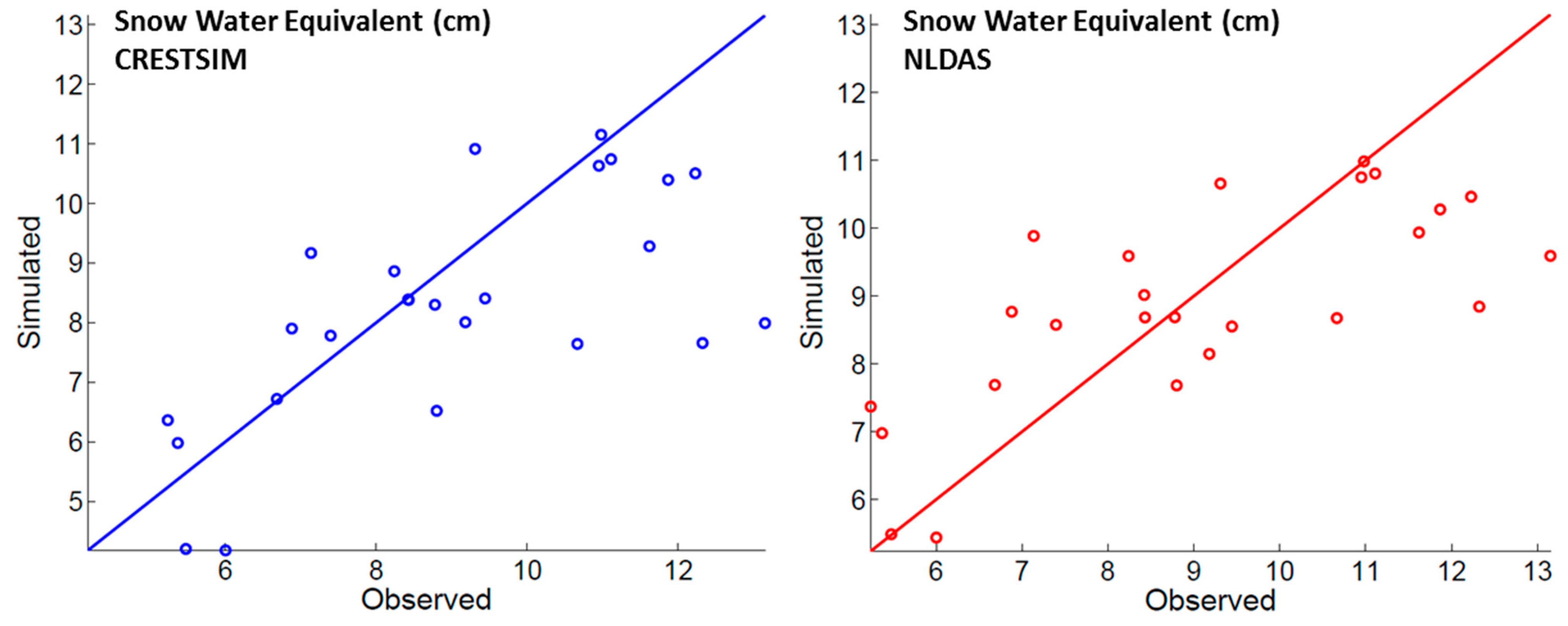
The snow water equivalent time series (Figure 6) also showed a good agreement in the accumulation period (before March) but some underestimation in the later period (after late February, Figure 6 and Figure 7). The SWE underestimation in that second period explains the similar behavior the snow depth had for the same period (Figure 4). Additionally, it was observed that before the snowpack warmed to an isothermal state 0 °C, the difference between observed SWE and the modeled data was minimal. The statistics for snow water equivalent (Table 3) still showed that SNTHERM is an adequate model for simulating this land surface process even if it is forced with NLDAS assimilated data.

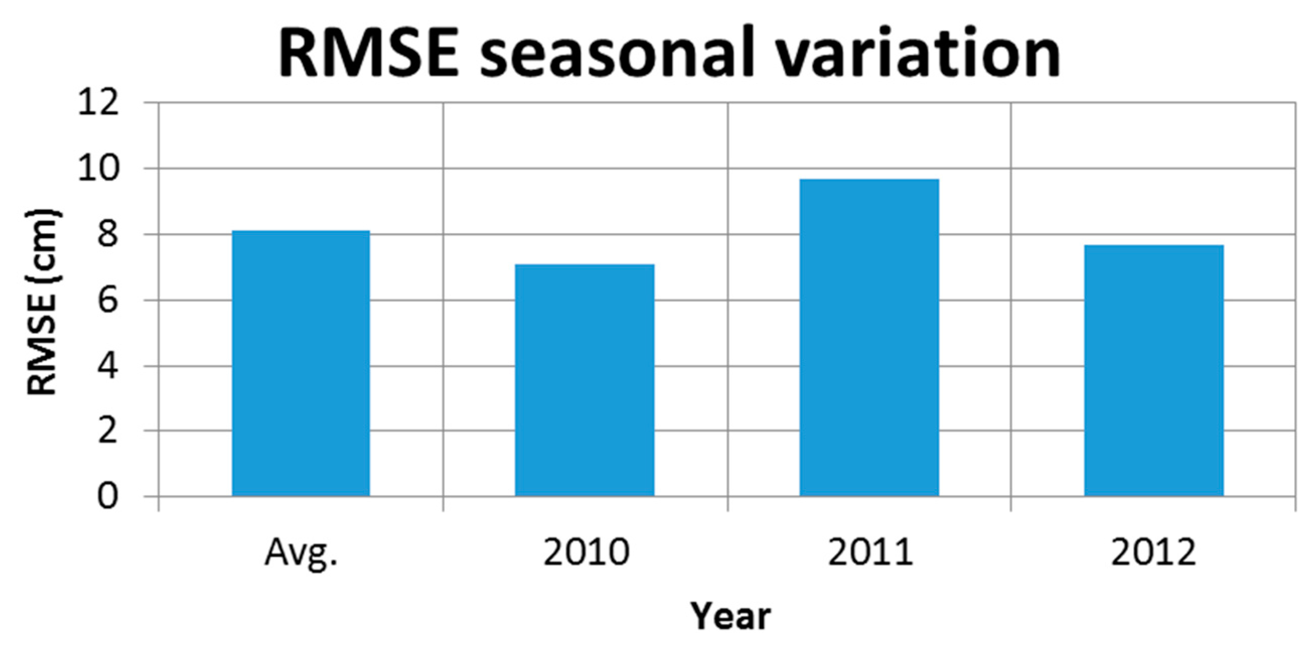
The results for the three simulated winters were considered good when tested for efficiency measurements. Figure 8 shows the variation of the snow depth RMSE for all simulated winters, being the first bar the RMSE average for all simulated winters. The RMSE values are always below 10 cm, which is less than fifty percent of the standard deviation. RMSE values less than half of the standard deviation along with the KGE and R² values observed on Table 3 are considered a good simulation.

Figure 6. Time series for 2011–2012 winter. Snow water equivalent (cm). Legend: manual CREST-SAFE Observations (Observed), NLDAS meteorological data simulation (NLDAS), and CREST-SAFE meteorological data simulation (CRESTSIM).

Figure 6. Time series for 2011–2012 winter. Snow water equivalent (cm). Legend: manual CREST-SAFE Observations (Observed), NLDAS meteorological data simulation (NLDAS), and CREST-SAFE meteorological data simulation (CRESTSIM).

Figure 7. SWE Scatter Plot (winter 2011–2012) for both simulated scenarios: (left) CRESTSIM; and (right) NLDAS.

Figure 7. SWE Scatter Plot (winter 2011–2012) for both simulated scenarios: (left) CRESTSIM; and (right) NLDAS.

Figure 8. Seasonal variation of the RMSE for simulated snow depth. The first bar is the average RMSE for all simulated winter seasons. The other bars are the RMSE of each particular simulated winter season.

Figure 8. Seasonal variation of the RMSE for simulated snow depth. The first bar is the average RMSE for all simulated winter seasons. The other bars are the RMSE of each particular simulated winter season.

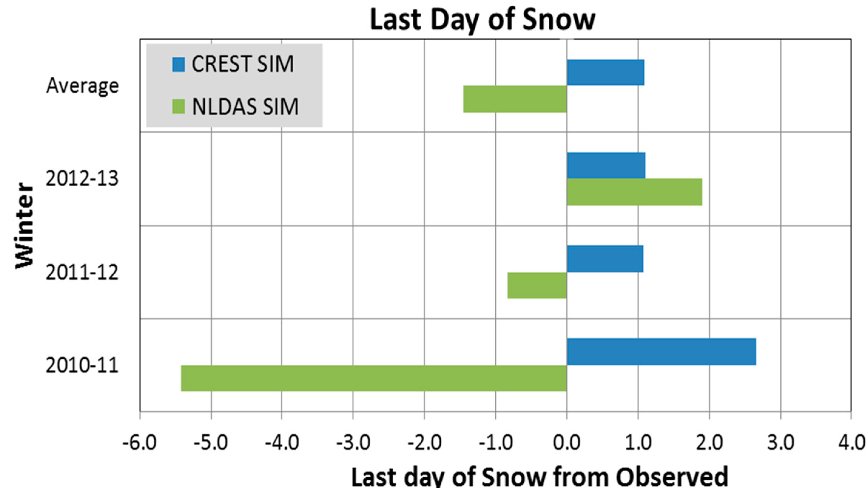
5.2. Last Day of Snow

The last day of snow is defined by the National Oceanic and Atmospheric Administration (NOAA) and United States Geological Survey (USGS) as the last day of measurable snow (that is, greater than a trace), which is approximately 3 cm. This threshold was defined based on the detection threshold on most automatic snow depth sensors and remote sensing binary products (snow and no-snow detection). It is a very interesting variable mainly because it is a good measurement of model performance in the melting period and it is a very important parameter to discretize the “snow and no-snow” mask for snow remote sensing.

Figure 9 shows the model performance in the different simulated years. The plot’s top part shows that, on average, the model melts the snow within the ±1.3 days of the actual snow disappearance, which can be considered fair to good timing for most hydrological applications.

Figure 9. Last day of snow. This plot assumes the last day of snow as the 1st day of observed snow depth under 3 cm. Zero is the observed last day of snow and the bars represent the time difference between the simulated and observed last day of snow.

Figure 9. Last day of snow. This plot assumes the last day of snow as the 1st day of observed snow depth under 3 cm. Zero is the observed last day of snow and the bars represent the time difference between the simulated and observed last day of snow.

5.3. Snowpack Temperature

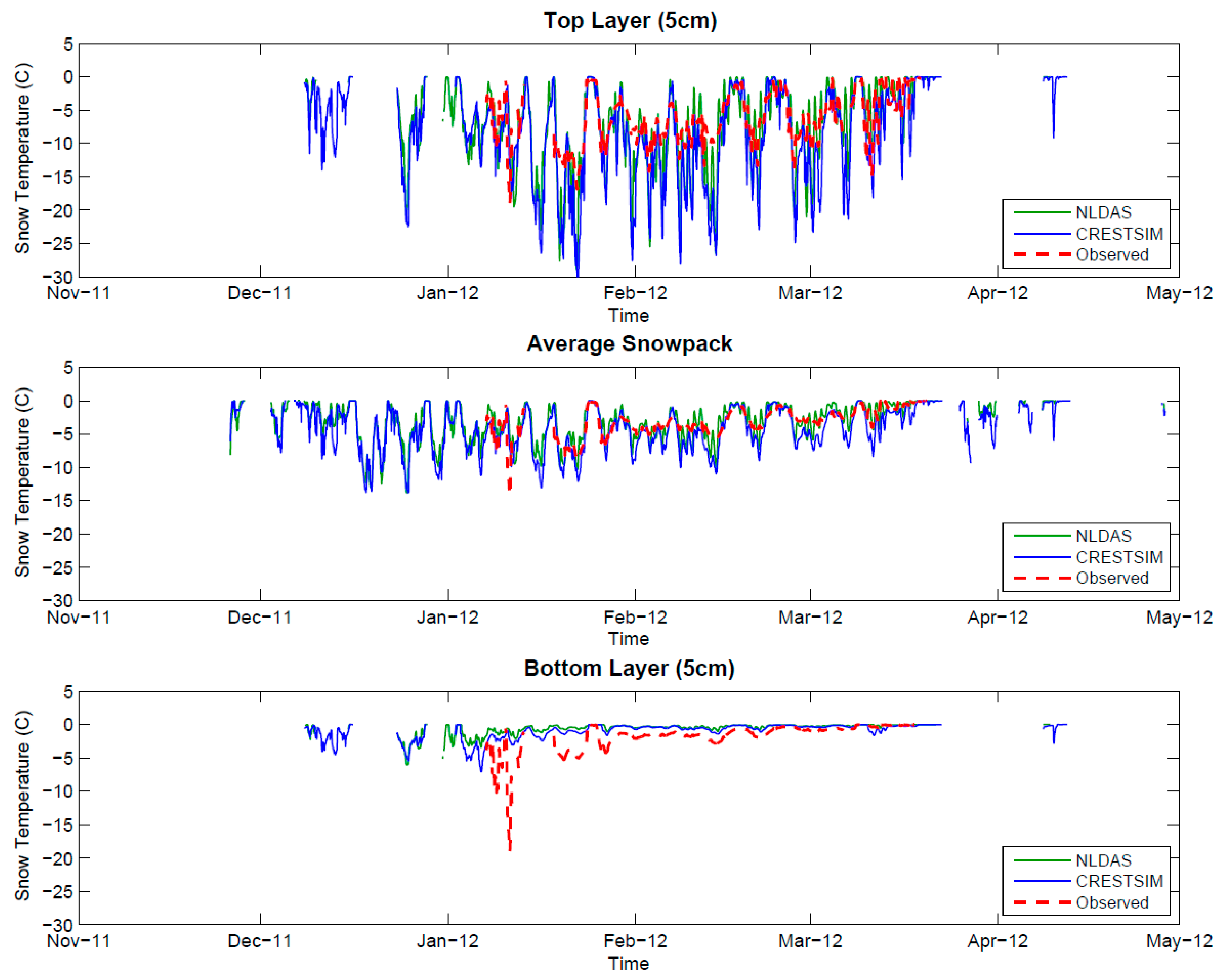
Figure 10 shows the temperature for top layer, bottom layer, and average temperature of the snowpack. The top layer is the most influenced layer by the climatic conditions (air temperature, wind, and solar radiation). As expected, there are lower temperatures in the top and average layers of the snowpack relative to the bottom layer. This is explained by the lagging effect that the upper layers of the snowpack have over the lower layers (lag in the energy transfer between layers), which increases with the increase of the overall snowpack depth.

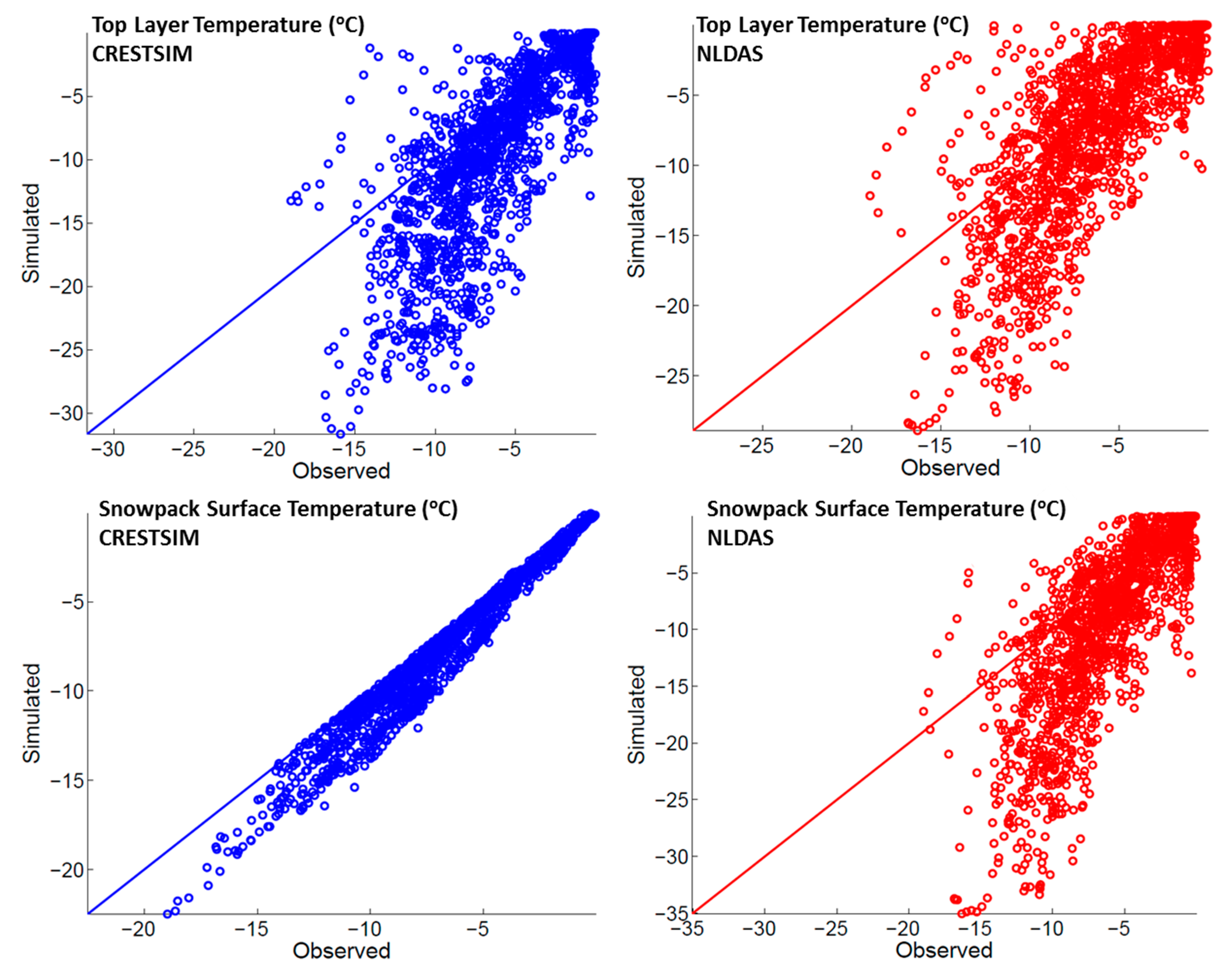
The observed and simulated temperatures in the top layer showed a similar behavior for both simulated scenarios (Figure 11, top). However, the observed temperature showed less variability characterized by a lower standard deviation. This implies that even in the first 5 cm of the snowpack, there is a temperature dampening effect. It also indicates that the model snow layers heat loss/gain process is represented but overestimated within the snowpack.

On the other hand, the bottom layer simulated temperature, which is less influenced by the meteorological conditions, showed less variability than the observed temperatures at that same depth. This is especially true when snow depth is less than 40 cm in the accumulation period (before February).

Figure 10. Time series for temperature (°C) in the top layer (upper), average (middle), and bottom layer (lower) of the snowpack. Legend: NLDAS meteorological data simulation (NLDAS), CREST-SAFE meteorological data simulation (CRESTSIM), and manual CREST-SAFE Observations (Observed).

Figure 10. Time series for temperature (°C) in the top layer (upper), average (middle), and bottom layer (lower) of the snowpack. Legend: NLDAS meteorological data simulation (NLDAS), CREST-SAFE meteorological data simulation (CRESTSIM), and manual CREST-SAFE Observations (Observed).

Figure 11. Scatter plot for top layer snowpack temperature (top) and snowpack surface temperature (bottom) for both simulated scenarios: (left) CRESTSIM and (right) NLDAS.

Figure 11. Scatter plot for top layer snowpack temperature (top) and snowpack surface temperature (bottom) for both simulated scenarios: (left) CRESTSIM and (right) NLDAS.

Regarding the average snowpack temperature, statistics on Table 4 show that the agreement between observed and simulated temperatures was fair, but the t-test results demonstrate that there are significant differences between the averages of the compared variables. Consequently, the simulation was not satisfactory within acceptable tolerances.

Table 4. Statistics for overall snowpack temperature (°C). Validation period: Winter 2011–2012. Rows definitions are same as in Table 3. The number of observations was 2030.

Statistic	Snowpack Average Temperature
	Observed	CRESTSIM	NLDAS
Mean	−3.26	−4.27	−3.07
Max	−0.01	−0.03	−0.03
SD	2.11	2.74	2.37
RMSE	-	2.06	1.64
R2	-	0.57	0.55
KGE	-	0.61	0.63
t	-	11.39	−2.40

Table 4. Statistics for overall snowpack temperature (°C). Validation period: Winter 2011–2012. Rows definitions are same as in Table 3. The number of observations was 2030.

Statistic	Snowpack Average Temperature
	Observed	CRESTSIM	NLDAS
Mean	−3.26	−4.27	−3.07
Max	−0.01	−0.03	−0.03
SD	2.11	2.74	2.37
RMSE	-	2.06	1.64
R2	-	0.57	0.55
KGE	-	0.61	0.63
t	-	11.39	−2.40

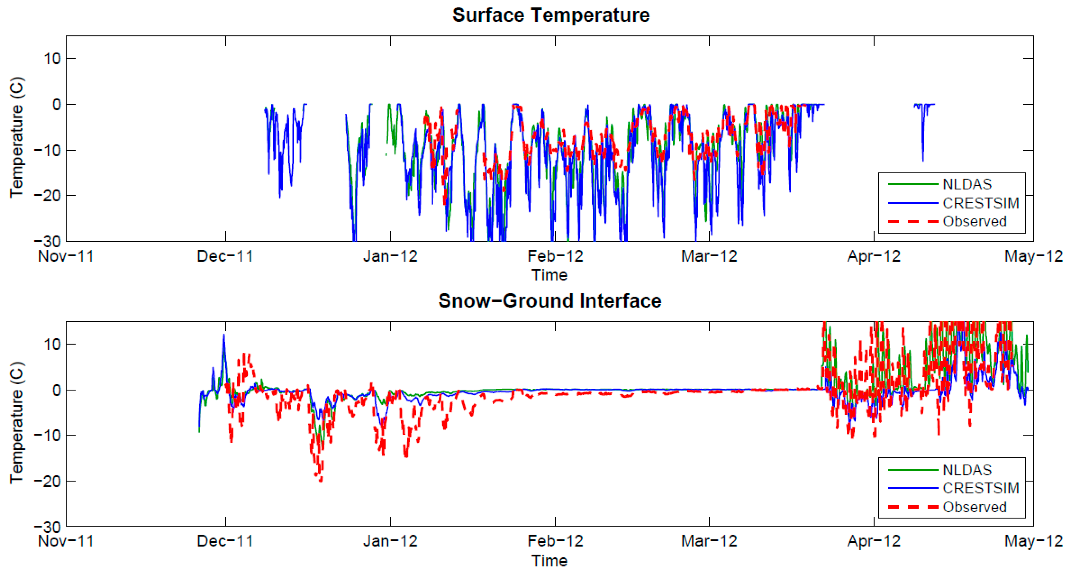
Results also indicated that the model successfully captured the variability of the temperature at the snowpack surface (Figure 11 and Figure 12). This conclusion is supported by the statistics which showed a good model performance, especially when using observed meteorological data (Table 5). However, statistical results also indicated that the model did not simulate the snowpack temperature effectively for the snow-ground interface. The snow-ground interface is the theoretical boundary layer of the snowpack which separates the snow from the ground. The temperature at this layer is a direct representation of how the model is simulating the heat transfer between the soil and the snowpack. This confirms the aforementioned hypothesis of the model poorly predicting the energy gains and losses throughout the snowpack.

Figure 12. Time series for temperature (°C) in the surface (upper) and snow-ground interface (lower) snowpack boundaries. Legend: NLDAS meteorological data simulation (NLDAS), CREST-SAFE meteorological data simulation (CRESTSIM), and manual CREST-SAFE observations (Observed). Validation period: Winter 2011–2012. The number of observations was 975 for top and 2030 for bottom.

Figure 12. Time series for temperature (°C) in the surface (upper) and snow-ground interface (lower) snowpack boundaries. Legend: NLDAS meteorological data simulation (NLDAS), CREST-SAFE meteorological data simulation (CRESTSIM), and manual CREST-SAFE observations (Observed). Validation period: Winter 2011–2012. The number of observations was 975 for top and 2030 for bottom.

Table 5. Statistics for surface and snow-ground interface snowpack temperatures (°C). Validation period: Winter 2011–2012. Row definitions are same as in Table 3. The number of observations was 2030 and 975 respectively.

Statistic	Snow Surface Temperature			Snow-Ground Interface Temperature
	Observed	CRESTSIM	NLDAS	Observed	CRESTSIM	NLDAS
Mean	−6.43	−7.39	−9.75	−6.43	−1.03	−0.03
Max	−0.01	−0.04	−0.01	−0.01	0.14	0.14
SD	3.83	4.51	7.64	3.83	1.11	0.18
RMSE	-	1.39	6.29	-	6.36	7.47
R2	-	0.97	0.58	-	0.29	0.00
KGE	-	0.85	0.35	-	0.26	0.00
t	-	6.1	15.0	-	−52.2	−64.7

Table 5. Statistics for surface and snow-ground interface snowpack temperatures (°C). Validation period: Winter 2011–2012. Row definitions are same as in Table 3. The number of observations was 2030 and 975 respectively.

Statistic	Snow Surface Temperature			Snow-Ground Interface Temperature
	Observed	CRESTSIM	NLDAS	Observed	CRESTSIM	NLDAS
Mean	−6.43	−7.39	−9.75	−6.43	−1.03	−0.03
Max	−0.01	−0.04	−0.01	−0.01	0.14	0.14
SD	3.83	4.51	7.64	3.83	1.11	0.18
RMSE	-	1.39	6.29	-	6.36	7.47
R2	-	0.97	0.58	-	0.29	0.00
KGE	-	0.85	0.35	-	0.26	0.00
t	-	6.1	15.0	-	−52.2	−64.7

The standard deviation (SD) was much higher in the simulations than in the observed data for the snow surface temperature. This means that the energy losses and gains of the simulated snowpack are higher than they should be. In other words, when the air temperature drops, the model draws more energy from the snowpack that it should, particularly in very low temperatures (lower than −15 °C). Thus, adjustments to the energy transfer of snow layers could improve the model performance, particularly for the top layer.

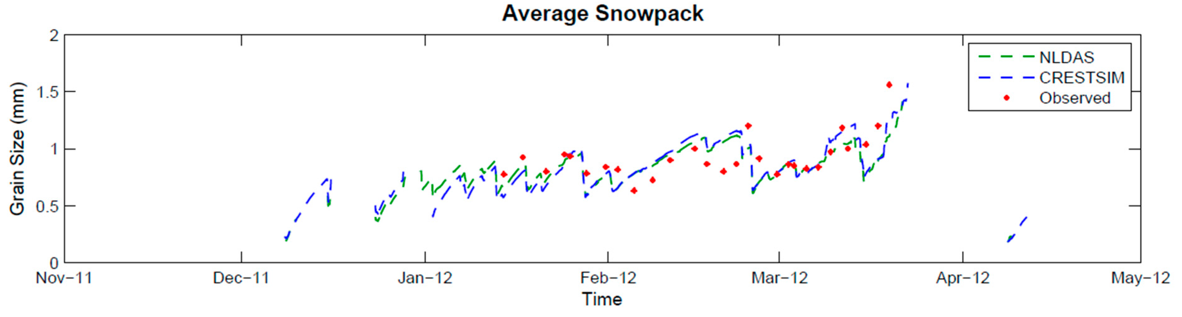
5.4. Snowpack Grain Size

Snow grain size is important to accurately predict snow depth and SWE using microwave remote sensing. Differences between the observed and simulated snow grain size are associated with the manual method (microscope) used to estimate in situ snow grain size, which represents the average size of several grains collected in a random sample. The accuracy of this measurement has been questioned [56] and it is hypothesized to be the cause of the discrepancies between observations and simulations. Even though, Figure 13 and Figure 14 depicts that observed and simulated grain size are within range. However, the 3 simulated years showed major disagreements, mainly occurring during the warm periods.

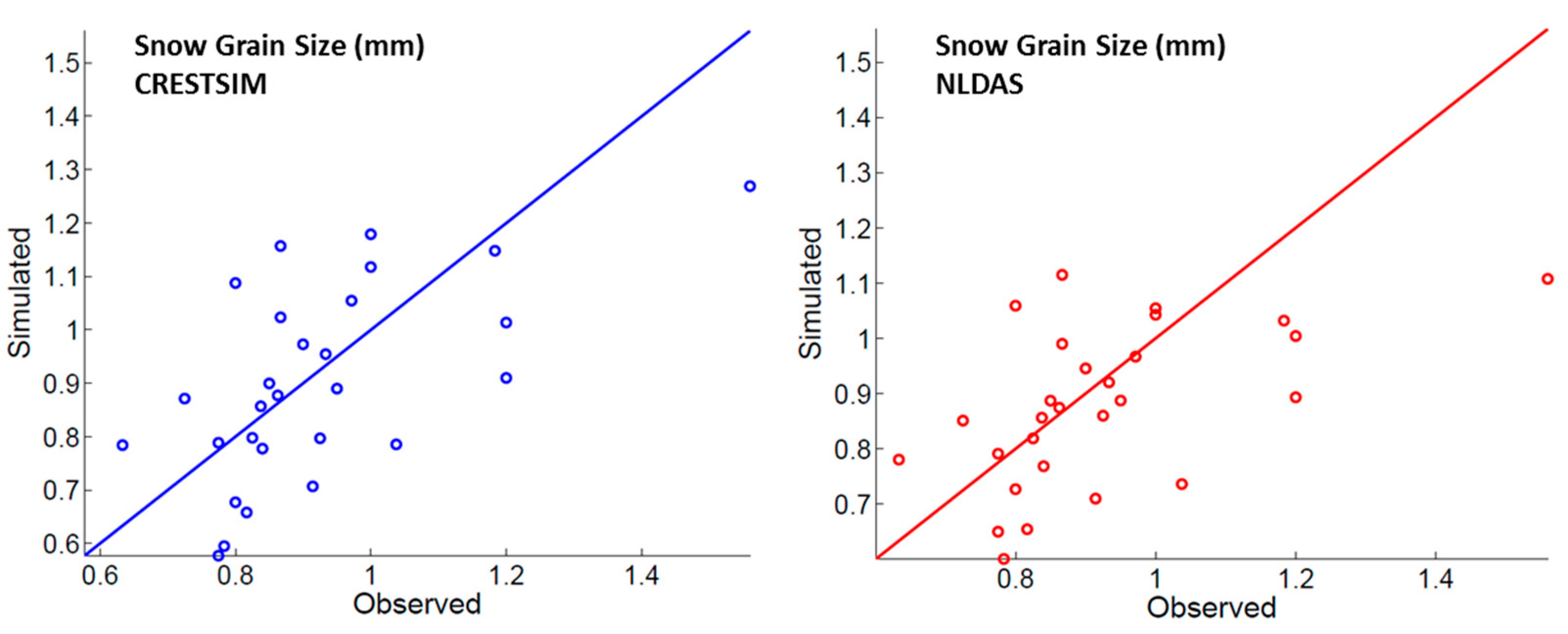
Both simulated scenarios (CRESTSIM and NLDAS) failed the efficiency tests. Nonetheless, the disagreement in part can be explained with the uncertainties associated with the manual observations (including human error) of grain size, in particular during the snow isothermal state.

Figure 13. Time series for grain size (mm). Legend: NLDAS meteorological data simulation (NLDAS), CREST-SAFE meteorological data simulation (CRESTSIM), and manual CREST-SAFE observations (Observed).

Figure 13. Time series for grain size (mm). Legend: NLDAS meteorological data simulation (NLDAS), CREST-SAFE meteorological data simulation (CRESTSIM), and manual CREST-SAFE observations (Observed).

Figure 14. Snow grain size scatter plot (winter 2011–2012) for both simulated scenarios: (left) CRESTSIM; and (right) NLDAS.

Figure 14. Snow grain size scatter plot (winter 2011–2012) for both simulated scenarios: (left) CRESTSIM; and (right) NLDAS.

Statistics on Table 6 show that the average variability of the observed grain size was not well captured by the model (low correlational coefficient) and the RMSE is as high as the standard deviation. These results indicate poor model efficiency for this particular parameter. Adjustments are recommended to the grain size growth algorithm, before simulations results can be used as input for radiative transfer models (RTMs) and other remote sensing applications. However, in recent years many improvements have been made to reduce the uncertainties associated with snow grain size simulations [57]. Most improvements are based on snow age, snow temperature, and the snow temperature gradient. These improvements can easily be incorporated into SNTHERM.

Table 6. Grain size statistics. Validation period: Winter 2011–2012. Row definitions are same as in Table 3. The number of observations was 29.

Statistic	Snowpack Average Grain Size
	Observed	CRESTSIM	NLDAS
Mean	0.923	0.901	0.878
Max	1.560	1.269	1.115
SD	0.185	0.183	1.143
RMSE	-	0.164	0.167
R2	-	0.357	0.278
KGE	-	0.60	0.49
t	-	0.441	1.010

Table 6. Grain size statistics. Validation period: Winter 2011–2012. Row definitions are same as in Table 3. The number of observations was 29.

Statistic	Snowpack Average Grain Size
	Observed	CRESTSIM	NLDAS
Mean	0.923	0.901	0.878
Max	1.560	1.269	1.115
SD	0.185	0.183	1.143
RMSE	-	0.164	0.167
R2	-	0.357	0.278
KGE	-	0.60	0.49
t	-	0.441	1.010

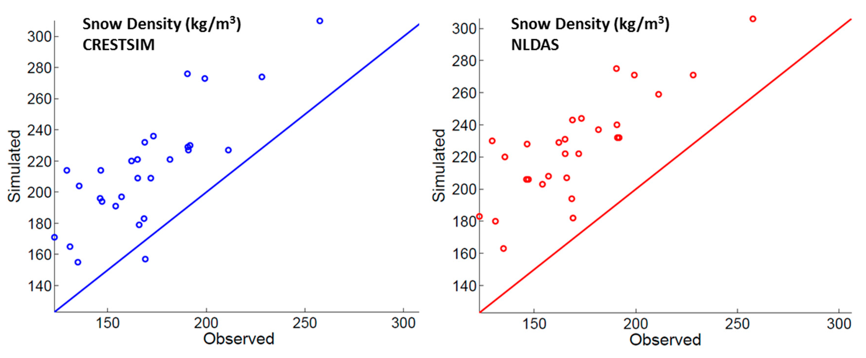
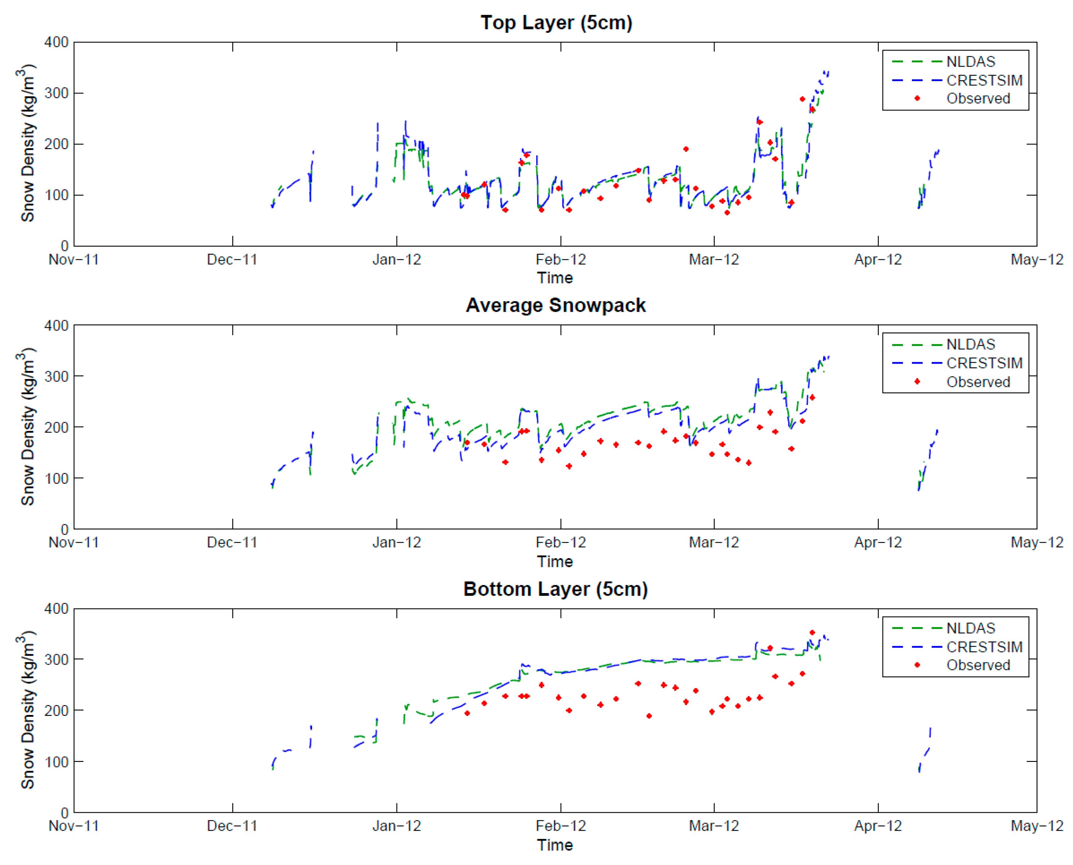
5.5. Snowpack Density

The simulated values of snow density were close to the observed values (Figure 15 and Figure 16). The top layer density was in better agreement relative to the bottom layer, in which density was overestimated by the model as shown in the statistics presented in Table 7. This indicates that algorithm from is working better at the top layer and failing for the overburden, which is the most influential phenomenon in the bottom layer. Is also important to notice that there are some sudden peaks in the simulation that are hard to explain and that could be caused by sudden peaks in the snow temperature, melting events or the presence of wet snow.

Figure 15. Average snow density scatter plot (winter 2011–2012) for both simulated scenarios: (left) CRESTSIM and (right) NLDAS.

Figure 15. Average snow density scatter plot (winter 2011–2012) for both simulated scenarios: (left) CRESTSIM and (right) NLDAS.

Figure 16. Time series for snow density (kg/m³) in the top layer (upper), average (middle), and bottom layer (lower) of the snowpack. Legend: NLDAS meteorological data simulation (NLDAS), CREST-SAFE meteorological data simulation (CRESTSIM), and manual CREST-SAFE observations (Observed). The number of observations was 29.

Figure 16. Time series for snow density (kg/m³) in the top layer (upper), average (middle), and bottom layer (lower) of the snowpack. Legend: NLDAS meteorological data simulation (NLDAS), CREST-SAFE meteorological data simulation (CRESTSIM), and manual CREST-SAFE observations (Observed). The number of observations was 29.

Table 7. Snow density (kg/m³) statistics for bottom layer and top layer. Validation period: winter 2011–2012. Row definitions are same as in Table 3. The number of observations was 29.

Statistic	Snowpack Density
	Top Layer			Bottom Layer			Average
	Observed	CRESTSIM	NLDAS	Observed	CRESTSIM	NLDAS	Observed	CRESTSIM	NLDAS
Mean	129.66	127.92	126.18	234.62	292.30	289.26	169.86	214.79	225.86
Max	287.50	286.19	241.16	352.78	328.81	322.06	257.56	310.00	306.0
SD	60.25	43.831	38.43	36.08	25.99	21.09	30.74	36.89	32.183
RMSE	-	40.553	35.01	-	65.64	62.71	-	49.92	59.12
R2	-	0.53	0.69	-	0.261	0.25	-	0.64	0.66
KGE	-	0.70	0.62	-	0.31	0.24	-	0.66	0.57
t	-	0.126	0.262	-	−6.86	−6.92	-	−4.95	−6.66

Table 7. Snow density (kg/m³) statistics for bottom layer and top layer. Validation period: winter 2011–2012. Row definitions are same as in Table 3. The number of observations was 29.

Statistic	Snowpack Density
	Top Layer			Bottom Layer			Average
	Observed	CRESTSIM	NLDAS	Observed	CRESTSIM	NLDAS	Observed	CRESTSIM	NLDAS
Mean	129.66	127.92	126.18	234.62	292.30	289.26	169.86	214.79	225.86
Max	287.50	286.19	241.16	352.78	328.81	322.06	257.56	310.00	306.0
SD	60.25	43.831	38.43	36.08	25.99	21.09	30.74	36.89	32.183
RMSE	-	40.553	35.01	-	65.64	62.71	-	49.92	59.12
R2	-	0.53	0.69	-	0.261	0.25	-	0.64	0.66
KGE	-	0.70	0.62	-	0.31	0.24	-	0.66	0.57
t	-	0.126	0.262	-	−6.86	−6.92	-	−4.95	−6.66

The main parameter controlling the compaction rate of snow by overburden is snow viscosity (eta0 on Table 2). This parameter was selected for calibration partly because of the uncertainties associated with the value used expressed by Jordan 1991 [12]. The calibration process optimized the value for “eta0” on the CREST-SAFE, considering geographical and seasonal influences. Even though the parameter was adjusted, the overestimation of snowpack densities was also shown in the snowpack average values. Consequently, further adjustments to the overburden algorithm are recommended to achieve additional improvements in the simulations.

6. Conclusions

In this phase of the CREST-SAFE research, the evaluation of the SNTHERM on a point scale was performed. Meteorological data from CREST-SAFE and NLDAS assimilation system were used as input parameters to the SNTHERM model. The snowpack properties from both simulations were analyzed to assess the overall model capabilities and potential to produce both input datasets for hydrological models and datasets for remote sensing snow product calibration and validation.

Better parameterization for model initialization increases the accuracy of the model. In this work, the majority of the simulations with in situ weather forcing measurements produced better results than simulations performed with NLDAS assimilated meteorological data. This is true for snowpack physical properties such as snow depth, snow water equivalent, grain size, and temperature. However, NLDAS simulations were generally acceptable and the results of the quantitative assessments (i.e., KGE) performed with the simulated scenarios were similar. This is especially true for snow depth, snow water equivalent, snow density, and average last day of snow. This indicates that for hydrological modeling and binary snow remote sensing (snow and no-snow detection), the SNTHERM model forced with NLDAS meteorological data can provide results within acceptable tolerances.

Layered snowpack information is of great interest for snow remote sensing products and hydrological modeling. The simulations results confirmed that the lag in the energy transfer that the snowpack upper layers have over the lower layers is very important. Failing to capture this effect in the simulations could lead to large errors in the results. However, the SNTHERM model successfully captured the variability of the temperature at the surface. On the other hand, the model did not perform as well for the middle and lower snowpack layers.

For snow grain size, statistical analysis shows that the variability of the observed grain size was not well captured by the model, as represented by a low correlational coefficient. Consequently, adjustments are recommended to the grain size growth algorithm. In the same manner, based on the results obtained in this work, the SNTHERM model’s algorithm could be modified to further improve its performance for simulating these aforementioned snowpack physical properties. The steps recommended include adjusting the heat transfer coefficients within the snowpack layers, then adjusting the snow compaction rate by overburden, and finally adjusting grain size exponential growth coefficients.