Petrophysical Characterization of Non-Magnetic Granites; Density and Magnetic Susceptibility Relationships

Abstract

In this work we establish reliable correlations between density and magnetic susceptibility in three paramagnetic granites from the Pyrenees. In total, 128 sites (310 density measurements and >2600 susceptibility ones) were studied in the Mont Louis-Andorra, Maladeta and Marimanha granitic plutons covering the main range of variability of magnetic susceptibility. Regressions were calculated for every granitic body and an integrated linear function was obtained for the entire dataset: ρ (kg/m³) = 2566 (kg/m³) + 0.541κ (10⁻⁶ S.I.) (R:0.97). This relationship is only valid in the paramagnetic domain, where iron is mostly fractioned in iron-bearing phyllosilicates and the occurrence of magnetite is negligible (or at least its contribution to the bulk susceptibility). This relationship, likely different in other bodies, allows for transforming magnetic susceptibility data into density data, helping to constrain gravity modelling when density data from rock samples are scarce. Given the large amount of AMS studies worldwide, together with the quickness and cost-effectiveness of susceptibility measurements with portable devices, this methodology allows for densifying and homogenizing the petrophysical data when modelling granite rock volumes based on both magnetic and gravimetric signals.

1. Introduction

Beyond classic mineral exploration in hydrothermally altered or contact metamorphism rocks (e.g., Joly et al. [1]; Dentith and Mudge [2]) or as radioactive waste disposals (e.g., Wang [3]), geophysical surveying of granite bodies is increasingly of interest due to, among other aspects, their potential in geothermal energy (Genter et al. [4] Huenges and Ledru [5]; Moore et al. [6]; Zhang and Zhao [7]). Potential fields geophysical techniques, both gravity and magnetism, have been of great help for 2D and 3D modeling of granitic bodies for a long time (Bott et al. [8]; Bott and Smithson [9], Henkel [10] Vigneresse [11] Ameglio et al. [12]; Cruz et al. [13]) inasmuch they are quick, repeatedly resolute and cost-effective methods for an initial characterization of those bodies at depth. As in any potential-field study, petrophysical data are an essential constraint to link the geophysical signal with the geological features, and thus a keystone to reduce the ambiguity and uncertainty in the interpretations (Henkel [10,14,15]; Enkin et al. [16]; Dentith et al. [17]; Pueyo et al. [18]).

Density and susceptibility relationships have been well-known in granitic rocks from a petrological and petrophysical point of view since the pioneering works by Henkel ([10,14]). Some works have demonstrated that δ¹⁸O and the wt.% SiO₂ display a negative correlation to magnetic susceptibility in granites (Ellwood and Werner [19], Villaseca et al. [20] respectively). Moreover, it is well known that the magnetic properties of granites depend on their chemical and tectonic affinity (Kanaya and Ishihara [21]; Ishihara [22], 1981 [23]) and they are classified as magnetic granites (κ ranging from 10⁻³ to 10⁻² S. I.) and non-magnetic granites (κ from 10⁻⁵ to 10⁻⁴ S.I.) (Ellwood & Werner [19]). Non-magnetic granites usually correspond to supracrustal sources, S-type (Chappell & White [24]), where iron is fractionated mainly in ilmenite (paramagnetic at room temperature) and biotite (strongly paramagnetic; Martín-Hernández & Hirt [25]). In magnetic granites, usually related to deeper and/or igneous sources (I-type), the iron mainly forms magnetite crystals (ferrimagnetic). Elming [26] in the Caledonides of Jämtland (Sweden), or more recently Terrinha et al. [27] in Sintra granite, showed coarse relations between density and magnetic susceptibility along five orders of magnitude (κ from 10⁻⁵ to 10⁻¹ S.I.). Criss and Champion [28] measured the density in paleomagnetic samples of the Idaho granite and recognized that variations in susceptibility were mostly related to the rock density at a regional scale. Bourne [29] stablished that density and magnetic susceptibility (separately) inversely correlate with SiO₂ concentrations in ferromagnetic granites (ca. κ > 500 × 10⁻⁶ S.I.; Bouchez [30,31]).

A big step further was given by Gleizes [32]; Bouchez et al. [33]; Gleizes et al. [34] and in the Foix and Mont-Louis Andorra granites, respectively (in the Axial Zone of the Pyrenees). Gleizes et al. [34] related the magnetic susceptibility with the iron composition [Fe⁺² and Fe⁺³] and the expected susceptibility derived from theoretical estimates (after Rochette [35] and Rochette et al. [36]), and also proposed a correlation between magnetic susceptibility and magmatic facies in paramagnetic granites (ca. κ < 500 × 10⁻⁶ S.I). Their work has had a profound impact in the application of anisotropy of magnetic susceptibility (AMS) techniques to characterize the internal structure and composition of granitic bodies. Currently, hundreds of granitic bodies all over the world have been systematically studied by AMS, helping us to understand their emplacement models and generating vast databases of susceptibility data (Román-Berdiel et al. [37]; Aranguren et al. [38]; Trindade et al. [39]; Sant’Ovaia et al. [40]; Ferré et al. [41]; Kratinová et al. [42]; Joly et al. [43]; Porquet et al. [44] among many others).

Focusing only on paramagnetic granites (in terms of Bouchez [30], or on the paramagnetic trend (in terms of Henkel [15] and Enkin et al. [16]), very little has been done comparing these petrophysical properties. Ameglio et al. [12] and references therein) found fine correlations among density and magnetic susceptibility in a few samples from three calc-alkaline S-type (paramagnetic) granites from French and Spanish Variscan massifs (namely Sidobre, Cabeza de Araya and Mont Louis-Andorra).

In this paper, the main goal is to build reliable correlations between magnetic susceptibility and density in paramagnetic granites. Three plutons from the Pyrenees are the study-cases: Mont Louis-Andorra, Maladeta and Marimanha. Previous AMS studies in these bodies (Gleizes et al. [34]; Leblanc et al. [45]; Antolín-Tomás et al. [46], respectively) allow the conversion of a vast susceptibility database into robust and reliable density data ready to be modelled together with gravity signals.

2. Geological Setting

The granitic massifs of Maladeta (MAL), Marimanha (MAR) and Mount-Louis Andorra (MLA) crop out in the Axial Zone of the Pyrenees and belong to the tardi-tectonic granitic bodies of the Variscan Orogen (Figure 1). All three plutons were intruded in the upper crust during the latest stages of the Variscan orogeny (Gleizes and Bouchez [47]; Gleizes [32]; Leblanc et al. [45]; Antolín-Tomás [48]; Antolín-Tomás et al. [46]).

The Variscan belt of Europe is part of a vast Paleozoic chain built between 500 and 250 Ma, due to the convergence and collision of two large continental masses, Laurentia-Baltica and Africa (Matte. [49]). It is a sinuous orogen that can be followed discontinuously from the south of Spain (Martínez-Catalán [50]; Pastor-Galán et al. [51]) to the Bohemian massif, and which very probably extends under the Carpathians to the Variscan Caucasus (Figure 1A). It is therefore a Paleozoic chain of nearly 5000 km in length that constitutes the southwest edge of stable Europe (Matte [52]); 250 Ma ago, most of the Variscan belt was completely eroded and subsequent extension and formation of basins occurred during the Mesozoic (Pangea breakup). Then, in the Cenozoic, the Alpine orogeny developed a new collisional chain between Iberia and the SW margin of the Eurasian plate between 65 and 20 M.a. (e.g., Muñoz [52]) resulting in the current Pyrenean Mountain range. The Alpine orogeny gave rise to the uplift of Paleozoic units in the core of the Pyrenean range (i.e., the Axial zone) during the collision by developing a central antiformal stack of several southward-facing basement-involved thrust sheets (Muñoz [53]; Martínez-Peña and Casas-Sainz [54]; Casas et al. [55]). Recently, some authors claim that the persistence of a relatively flat envelope for the Paleozoic sedimentary pile and Variscan isograds, and the absence of Alpine crustal-scale faults in the core of the Axial Zone, suggest that the Axial Zone constitutes a large Variscan structural unit preserved during Pyrenean orogeny (Cochelin et al. [56]).

In this context, the Marimanha granite crops out within the Alpine Gavarnie/Nogueras thrust sheet, the uppermost unit of the south-verging piggyback-sequence in this part of the Pyrenees, whereas the Maladeta and Andorra-Mont-Louis granites, two of the largest granitic bodies of the Axial Pyrenees, crop out in the underlying Bielsa/Orri thrust sheet (Figure 1B).

During the Variscan orogeny, low-grade Paleozoic metasedimentary rocks were affected by progressive polyphasic deformation (Druguet [57], García-Sansegundo et al. [58], Casas et al. [59]), which mostly occurred during a compressional tectonic setting in which fold and thrust systems developed, giving rise to the crustal thickening of the Variscan cordillera in this region (Soula et al. [60]; Carreras and Capella [61], Gutierrez-Medina [62]; Clariana and García-Sansegundo [63]). Subsequently, in the last states of the variscan deformation, an extensional deformation event occurred. According to Soula [64]) and Autran [65]) the main deformation event is synchronous with the peak metamorphism, while other authors (Guitard [66], Zwart [67,68]; Liesa [69] and Aguilar [70]) consider the deformation event to have continued during and after the metamorphic peak. Early south-verging thrust sheets involve Silurian to Carboniferous rocks in the hanging wall and Cambro-Ordovician rocks in the footwall (e.g., Majesté-Menjoulas [71]; Raymond [72]; Bodin and Ledru [73]; Losantos et al. [74]). The Silurian slates act commonly as a detachment level between the two units, and the deformation above it is characterized by fault propagation folds affecting Silurian and Devonian rocks (García-Sansegundo [75], Clariana [76], Margalef [77]). The last stages of the variscan deformation have been characterized as dextral shear motion accompanied by granite intrusion (Leblanc et al. [78]; Evans et al. [79]; Gleizes et al. [80,81,82]; Olivier et al. [83]; Román-Berdiel et al. [84,85]; Auréjac et al. [86]). Due to crustal thickening, the Variscan segment of the Pyrenees experienced crustal flow, gneiss dome formation and subsequent granitic massifs intrusion in the upper crust by in- situ ballooning favored by the boundary between the Cambro-Ordovician and Siluro-Devonian rocks (Antolín-Tomás et al. [46]). The U–Pb ages published for the Pyrenean granites indicate that the Variscan plutonism of the Pyrenees is mainly Carboniferous (Romer and Soler [87]; Paquette et al. [88]; Guerrot [89,90]; Roberts et al. [91]; Maurel et al. [92]; Olivier et al. [93]; Gleizes et al. [82]) and Permian in age (Denèle et al. [94]). Recent works claim that partial melting, crustal flow, gneiss dome formation and pluton emplacement occurred over a very short period at the time scale of the Variscan belt formation, on the order of 5 Ma, at ca. 304 Ma (Denèle et al. [95]). In general, these magmatic bodies follow the dominant trend of the Variscan structure.

Figure 1. (A) European Variscan belt (Modified after Franke [96]); CZ-Cantabrian Zone, WALZ-West Asturian-Leonese Zone, GTOMZ-Galicia Tras-os-Montes Zone, CIZ-Central Iberian Zone, OMZ-Ossa Morena Zone, SPZ-Southportuguese Zone, PAZ-Pyrenean Axial Zone, CCR-Catalonian Coastal Ranges, NPM-Nord-Pyrenean Massifs, MB-Massifs Basques. (B) Geological sketch map of the Central part of the Pyrenees, showing the situation of the Pyrenean granites.

Figure 1. (A) European Variscan belt (Modified after Franke [96]); CZ-Cantabrian Zone, WALZ-West Asturian-Leonese Zone, GTOMZ-Galicia Tras-os-Montes Zone, CIZ-Central Iberian Zone, OMZ-Ossa Morena Zone, SPZ-Southportuguese Zone, PAZ-Pyrenean Axial Zone, CCR-Catalonian Coastal Ranges, NPM-Nord-Pyrenean Massifs, MB-Massifs Basques. (B) Geological sketch map of the Central part of the Pyrenees, showing the situation of the Pyrenean granites.

The Marimanha granite is a triangular pluton in map view, with an outcrop area of about 45 km². The available geochronological data for the Marimanha pluton consists of a poorly constrained Rb–Sr age (on whole rock) of 315–290 Ma (Palau i Ramirez [96]). At the petrological level, this massif includes gabbro, diorite, granodiorite and leucogranite facies (Palau i Ramirez [97]). Its intrusion occurred in the western end of the Pallaresa Dome, in Cambro–Ordovician siliciclastic metasediments, cutting the Silurian and Devonian limestones and slates involved in the Variscan Roca Blanca thrust (Losantos et al. [74]; Bodin and Ledru [73]). The metamorphic aureole overprints the Variscan structures, and the whole is cut by Late Variscan and/or Alpine WNW–ESE reverse faults.

The Maladeta granite massif (Evans [98]; Leblanc et al. [45]; Evans et al. [79]) is elongated in the E-W direction with an area of 400 km². Available geochronological data provide a rather young date of 277 ± 7 Ma (Rb/Sr; whole-rock, Vitrac-Michard et al. [99]). Petrographic zoning is defined in the western Aneto unit, with more basic rock-types surrounding others that appear to be more silicic, and the presence of gabbros is defined in the south-eastern part of the massif (Charlet [100,101]). The massif is penetratively deformed in some places near its southern edge, and major fault zones separate different units. It was emplaced into Cambro-Ordovician to Carboniferous rocks at a shallow level of about 6 km in depth (Pouget et al. [102]). It developed a contact metamorphism aureole in which the sillimanite grade has been reached.

The Mont-Louis-Andorra massif (Autran et al. [103]; Debon et al. [104]; Gleizes & Bouchez [47]; Gleizes et al. [34]; Bouchez and Gleizes [105]) is elongated in the E-W direction over 55 km and covers nearly 600 km². Recent available geochronological data provide an age of 301–303 Ma (U/Pb, Denèle et al. [95]). Petrographically, this massif consists of leucogranites, monzogranites and granodiorites with dioritic microgranular enclaves. Its intrusion occurred mainly in Ediacaran-Cambrian metasediments (Laumonier et al. [106]) and its top reaches Devonian sediments to the SW (Andorra). It developed a metamorphic contact aureole with isograds cutting across the regional metamorphic isograds (Guitard et al. [107]; Laumonier et al. [108]).

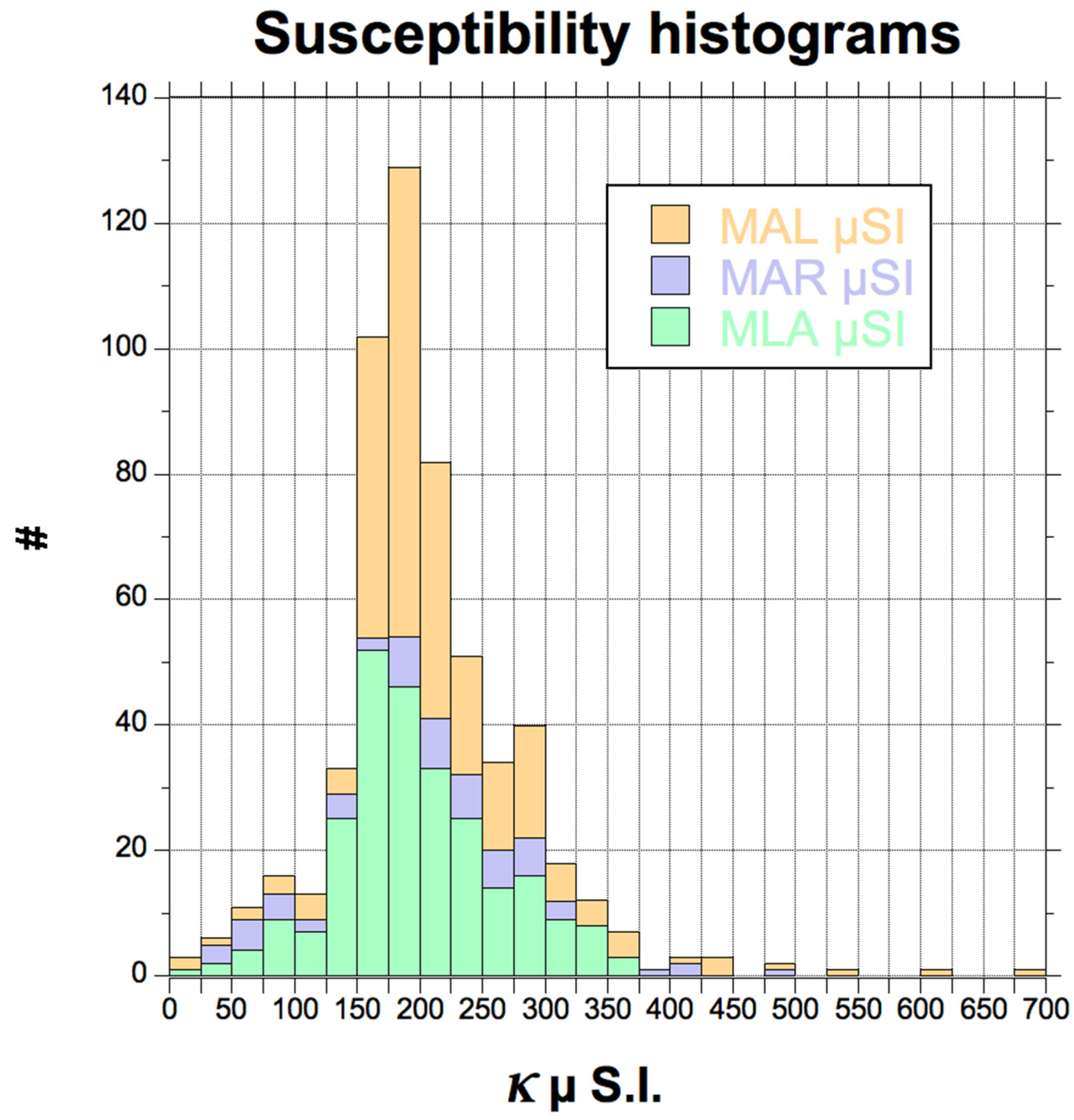
The bulk susceptibility from almost 600 studied AMS sites (Figure 2) displays very similar distributions for the three plutons and non-significant differences in the mean values (

Table 1. Main statistical variables from previous studies in Maladeta (MAL), Marimanha (MAR) and the Mont-Louis Andorra (MAL) granites (based on data by Leblanc et al., 1994 [45]; Antolín-Tomás et al. [46] and Gleizes et al. [34] respectively). O.S: Outcropping Surface, S. km²; sites per sq. km/. All susceptibility data are expressed as µ S.I. Note that these colors are kept all along the paper to refer those granites.

		Sites	O.S. (km2)	S./km2	min	Max	Mean	Median	RMS	Stan Dev	Stand Error	Skewness	Kurtosis
Maladeta	MAL	253	415	0.61	7	676	213.7	196.0	227.4	78.0	4.9	2.082	8.753
Marimanha	MAR	62	32	1.94	30	476	203.2	209.0	225.5	98.5	12.5	0.255	0.032
Mont Louis-Andorra	MLA	254	550	0.46	14	366	197.6	188.5	207.9	64.5	4.0	0.207	0.196
All	All	569	997	0.57	7	676	205.4	194.0	218.7	75.2	3.2	1.190	5.222

). These available and densely sampled nets of AMS data from the 90s and early 2000s (Figure 2) are revisited with new data acquired during the development of this work in the three granites to establish reliable correlations between density and magnetic susceptibility.

3. Methodology

In total, both properties (density and magnetic susceptibility) were studied in 128 sites from the Mont Louis-Andorra (MLA), Maladeta (MAL) and Marimanha (MAR) plutons (71, 42 and 15 sites, respectively) in the Central Pyrenees (Figure 3).

Four different types of samples were considered (Figure 4): (A) large hand samples of a few kilograms (type 1) were taken in 92 new sites (MLA and MAL plutons), (B) from them, subsampling of smaller blocks (mini-blocks; type 2; 20 to 200 g) were measured in 48 of those sites. (C) several previous samples from AMS studies (paleomagnetic standard specimens, type 3, about 25–30 g) were remeasured in 36 sites from MLA (21 sites; Gleizes et al. [33]) and MAR (15 sites; Antolín et al. [45]). Finally, (D) subsampling of some standard cores with a 0.5 cm Ø non-magnetic drill bit (1 cm in length, type 4-minicores, below 1 g) in the MLA granite allowed for the determination of susceptibility and other magnetic properties using vibrating and superconducting magnetometers. All the studied samples from these 128 sites tried to evenly cover the entire susceptibility spectra of the studied plutons (Figure 2).

3.1. Density Determinations

In type 1 samples (large hand blocks), the apparent density estimation was performed following the European standard UNE EN 1936:2006 (Natural stone test methods-Determination of real density and apparent density, and of total and open porosity [CEN/TC 246-Natural stones; CEN/TC 246/WG 2-Test methods]). More than two density data were taken in average per site (ranging between 1 and 5) at the IGME laboratories (Tres Cantos, Madrid), yielding a total of 95 determinations. Two main initial conditions must be honored: the specimens must be larger than 60 mL in volume, and their surface/volume ratio must range between 0.08 and 0.20 mm⁻¹ (regular cubes with sides between 30 and 75 mm). In the laboratory, the specimens are first dried in an oven at 70 ± 5 °C until a constant mass (m_D) is achieved; the difference between two consecutive weighing carried out after 24 h must be lower than 0.1% of the initial mass (this mass will also allow obtaining the dry bulk density). Then, the specimens are subjected to a vacuum of 2.0 (±0.7) kPa for 2 (±0.2) h. Distilled water is slowly added without losing the vacuum, and the samples are submerged more than 15 min. The water temperature should be 20 ± 5 °C. Atmospheric pressure is slowly restored and the samples are left 24 (±2) additional hours in water. Then, we proceed to the weighing of the specimens immersed in a hydrostatic balance (m_H) and subsequently dried with a damp cloth, and its saturated mass is determined (m_S). See additional details and instrumentation in Rubio et al. [1]).

Then the apparent (saturated) density is (in kg/m³):

ρ = ρ_W × m_D/([m_S − m_H])

(1)

where ρ_W is the density of distilled water at 20 °C: 988 kg/m³.

Type 2 samples (more than 80 mini-blocks) were measured in the University of Barcelona laboratories applying the Archimedes principle (without a previous drying and without using paraffin); part of this set was previously measured in the IGME laboratories in Madrid (as type 1 samples). In type 3 AMS samples (111 specimens from MAR), density was estimated in three different ways: using the Archimedes principle (samples with and without paraffin) and estimation of the rock volume with a Vernier caliper on cylindrical samples. Using this third method, 21 additional estimates from MLA were also taken. For that purpose, only regular (cylindrical sections) and complete samples (whole, unbroken, etc.) were used. Any broken, incomplete, irregular or cracked specimen was ruled out for this purpose. Apart from the weighting of the sample (m), the maximum and minimum diameters (Ø) and heights of the specimen (H) were measured with a Vernier caliper. Afterwards both measurements were averaged out (Ø_m and H_m) and the volume was rapidly calculated: V = π (Ø_m/2)²·H_m, as well as the density ρ = m/(π [Ø_m/2]²·H_m). Considering all types together, 310 density determinations were obtained; 69 in MAL, 130 in MLA and 111 in MAR plutons (

Table 2. Summary of new density and susceptibility measurements (depending upon the sample type) carried out in this paper, specifying laboratory procedures, instrumentation, mean values and standard deviation per granite pluton (see body text for further explanations). Groups/Labs: MAD: Madrid, BCN: Barcelona, ZAZ: Zaragoza, TLSE: Toulouse. Density measurements in kg/m³ and susceptibility in µ S.I.

Granite Body	Groups	Sample Type	Type	Weight	#Sites	#	Method	Mean	StaDev	Labs
Maladeta	ZAZ+MAD	Hand blocks	1	3–5 k	21	29	Archimedes+UNE	2685	63	MAD
Maladeta	BCN+MAD	Mini blocks	2	<20 g	21	40	Archimedes	2658	48	BCN+ MAD
Mont Louis-Andorra	ZAZ+MAD	Hand blocks	1	3–5 k	23	66	Archimedes+UNE	2670	47	MAD
Mont Louis-Andorra	BCN+MAD	Mini blocks	2	<20 g	27	43	Archimedes	2661	52	BCN+ MAD
Mont Louis-Andorra	ZAZ+TLSE	Pmag cores	3&4	≈25 g	21	21	Geometric	2657	54	ZAZ
Marimanha	ZAZ	Pmag cores	3	≈25 g	15	111	Archimedes w&w/o paraffine	2697	78	ZAZ
Total					128	310		2671	12
Granite body	#	KLY2/KLY3	Bartington	SM20	KT20	MPMSMVSM	Method	Mean	StaDev	labs
Maladeta	1134		38	1096			Field and Lab	171.9	131.9	MAD
Maladeta	126	90	36				Labs	187.0	155.9	BCN+ MAD
Mont Louis-Andorra	1059		40	591	428		Field and Lab	152.7	75.2	MAD
Mont Louis-Andorra	156	120	36				Labs	233.1	176.0	BCN+ MAD
Mont Louis-Andorra	48	21				27	Labs	192.5	94.4	ZAZ+ TLSE
Marimanha	106	106					Lab	232.5	133.9	ZAZ

).

3.2. Susceptibility and Rock Magnetism Measurements

In total, more than 2600 susceptibility determinations were obtained in 128 studied sites (Table 2). More than 80% were taken directly in 44 outcrops accompanying type-1 samples (21 selected sites from MAL and 23 ones from MLA plutons) using SM20 (1687 measurements) and KT20 (428 measurements) portable susceptometers (by GF Instruments and Terraplus, respectively). On average, more than 50 readings were measured in these outcrops (ca. 10–15 m²), and at least one large hand sample (type 1) was taken approximately in the center of the outcrop surface. Type 2 samples (>200 readings) were measured in a KLY-2 kappabridge located in the Paleomagnetic laboratory of the CCiTUB and Geociencias Barcelona (CSIC). Type 3 samples (paleomagnetic standard) were measured in susceptibility bridges available at the laboratories of the universities of Toulouse and Zaragoza (AGICO kappameters models KLY-2 and KLY-3, respectively). Selected specimens from Toulouse were measured again (1 per selected site) and contrasted to previously published works in the Mont Louis-Andorra granite (Gleizes et al. [34]). In the case of Marimanha, all available stored specimens at the Geotransfer Group (University of Zaragoza) were re-measured in some particular sites (Antolín et al. [46]; Rubio et al. [110]; Loi et al. [111]).

Finally, some comparisons between high (κ_HF) and low field (κ_LF) susceptibilities were performed using a MPMS superconducting magnetometer (model 5S by Quantum Design Ltd.) of the University of Zaragoza to determine the para- and ferromagnetic s.l. fractions. Selected cores from MLA pluton were re-measured in the KLY-3 and then subsampled. Those minicores (type 4 samples) were measured in the MPMS instrument under the same conditions as the AGICO instruments (external magnetic field of 0.4 mT, 4 Oe in AC at about 900 Hz) to obtain the low-field value (κ_LF). Eventually, the same minicores were subjected to two high DC fields (0.9 and 2.5 T), after the total magnetic saturation, to estimate the high-field paramagnetic susceptibility (κ_HF). Since the κ_HF only reflects the paramagnetic contribution, meaning κ_LF ≈ κ_HF, then a dominant paramagnetic contribution can be assumed. Otherwise, if κ_LF > κ_HF, then the ferromagnetic contribution cannot be neglected. Additionally, the same collection of mini cores was re-measured in a MVSM (model 3900 by Princeton Measurements Corporation) hosted in the CEREGE paleomagnetic laboratory at Aix-en-Provence while trying to characterize the ferromagnetic hysteresis as well as the high field (up to 1 T) response (paramagnetic slope).

4. Results

4.1. Paramagnetic Contribution to Bulk Susceptibility

Linear correlations of density and magnetic susceptibility have been only proven in a few samples from calc-alkaline (paramagnetic) granites from SE European Variscides (Ameglio et al. [12]). Therefore, the dominant paramagnetic contribution to the susceptibility must be firstly evaluated in our dataset. Standard laboratory measurements of magnetic (bulk) susceptibility are often taken with AGICO susceptometers at room temperature and low magnetic fields (0.4 mT or below, about 10 times larger than the Earth’s magnetic field) and depend on the contribution of all kinds of minerals (diamagnetic, paramagnetic and ferromagnetic). In non-magnetic granites (κ from 10⁻⁵ to 10⁻⁴ S.I. after Ellwood & Werner [19]) bulk susceptibility is reasonably assumed to be dominated by paramagnetic minerals (Bouchez [30]).

However, some previous comparisons of high-field and low-field susceptibilities in the Bielsa and Millares massifs (Román-Berdiel et al. [84,85], respectively) from the Pyrenees, near the studied plutons (see Figure 1B), attested to the occurrence of significant ferromagnetic fractions in the bulk susceptibility value: up to 20% and 40% in Millares and Bielsa, respectively (but never higher). Conversely, Marimanha data by Antolín et al. [46]), displayed a pure paramagnetic signal (Figure 5a).

Therefore, we run high-field and low-field susceptibility measurements on a set of representative samples (type 4) from the MLA pluton to unambiguously prove or disprove this assumption. The MPMS measurements confirm the pure paramagnetic behavior of the LF signal, since not a single analyzed sample from MLA gave any significant proportion of ferromagnetic components (Figure 5a). Besides, the induced magnetization measurements taken in the MVSM show a pure paramagnetic (linear) behavior and no significant ferromagnetic hysteresis (Figure 5b). Taking into account all of these results, together with the similar distribution of the magnetic susceptibility in the three studied granites (κ < 400 × 10⁻⁶ S.I. in 93% of the studied sites; Figure 6), we can extend this conclusion to our entire dataset and a generalized paramagnetic behavior can be assumed.

4.2. Data Distribution

The overall magnetic susceptibility distribution obtained in the analyzed samples (all types together) falls within the entire range of variability of the studied granitic bodies obtained in previous works (Gleizes et al. [34]; Leblanc et al. [45]; Antolín et al. [46], see Figure 2), as was originally designed. In Figure 6, only site means from the studied Pyrenean granites were plotted. The averages of the new susceptibility data (

Table 3. Synthesis of statistics of petrophysical data (density and susceptibility) obtained in this paper. Dens(ity) and Magnetic Sus(ceptibility) separately for each pluton, as well as the global means.

Variable	Min	Max	Points	Mean	Median	RMS	Std Dev	Std Error	Skewness	Kurtosis
Dens-MAL	2437	2821	48	2658	2660	2659	78	11	−0.445	0.594
Dens-MLA	2520	2797	65	2660	2659	2661	52	64	−0.264	0.849
Dens-MAR	2601	2865	15	2697	2691	2698	78	20	0.888	0.115
Density All	2437	2865	128	2664	2662	2664	66	59	−0.106	0.149
Sus-MAL	−13.2	762.5	45	204.5	169.1	257.6	158.3	23.6	19.781	41.531
Sus-MLA	−5.4	688.5	63	176.3	154	207.8	110.8	14	17.052	55.973
Sus-MAR	31.9	454.3	15	232.5	234.4	266.0	133.9	34.6	0.126	−12.126
Sus-All	−13.2	762.5	123	193.5	166.8	234.6	133.1	12	17.989	4.64

) mimic the mean from previous papers (Table 1). Therefore, our sampling can be considered representative for the studied bodies. Identically, the density distribution (again, only site means) also falls within the expected range of variability of granitic, syenitic, dioritic and gabbroic rocks (e.g., Dortman [112]; Schön [113]); 2500–2900 kg/m³.

The Henkel’s plotting (1976) of density versus magnetic susceptibility data for each pluton (MAL, MLA and MAR) (only site means) evinces, in the first instance, for noisy petrophysical relationships between both variables (Figure 7) with poor correlation coefficients. At this point, linear regressions are only reliable for the Marimanha pluton (R: 0.81), however, a deeper analysis must be performed and discussed, focusing on the sample types and their reliability.

5. Discussion

5.1. Noise in Magnetic Susceptibility and Density Measurements

Simple box-plots (Figure 8) of both variables and sample types separately attest for mean values relatively robust but also witnesses for several outliers in our dataset. These outliers reflect, in part, the extreme members of the observed variables, but not only. For example, the Maladeta susceptibility data seem to concentrate most of the outliers as well as the most extreme values found in the density distribution. It is worth noticing that the Marimanha pluton does not show any outlier.

The natural variability of the petrophysical properties in a given outcrop (site) as well as the type of samples used to characterized them are key variables to understand the noise in the Henkel’s plot (Figure 7). Magnetic susceptibility within an outcrop (ca. 10–15 m²) can easily spread along one order of magnitude or more. This behavior was already described, to a certain extent, in a homogeneity analysis at the meter and decameter scales performed in AMS sites of granites (Olivier et al. [114]). Density, at this scale, is much less variable in these rocks and hardly exceeds 1% in studies with 7 to 9 determinations per site (Loi et al. [111]; Rubio et al. [110]). In this sense, the total rock volume where both properties are measured is also critical. Type 3 samples are much smaller than type 1 (hand blocks), but since 9–15 standard specimens evenly distributed in the outcrop are measured (Enkin [115]; Pueyo et al. [116,117]), the total 90–150 cm³ rock volume measured at the site scale is comparable with type 1 samples but likely more representative since it covers a larger outcrop surface.

On the other hand, the comparison of susceptibility measurements from different instruments is not necessarily straightforward even in laboratory instruments (Sagnotti et al. [118]). Focusing on portable devices, few works have provided comparative analysis so far (Izquierdo-Llavall et al. [119]; Terrinha et al. [27];). Measuring settings (applied magnetic field and frequency) as well as coil diameters are not always the same and, therefore, measurements from different instruments are not necessarily comparable. This is similar to what happens with density determinations from different methods. For example, the geometric method for determining the sample volume in standard AMS or paleomagnetic samples used to underestimate the rock density. Assumable differences between 1–2%, depending upon the lithology, have been observed in Pyrenean rocks (Pueyo et al. [18]).

Therefore, the number and type of data in a given outcrop, as well as the instrumental and methodological approaches, are critical when attempting to ascertain the reliability and representativeness of the data, and thus they may represent significant sources of noise in the dataset. However, these issues are beyond the scope of this paper and should be tackled in future studies. Meanwhile, the experience gained in this study allows us to propose some best practices in the field and in the laboratory to improve the quality of the petrophysical characterization of granites:

−

Hand samples (type 1) are always desirable. Ideally, two–three samples of some dm³ each will allow obtaining some regular parallelepipeds in the laboratory (edges about 4–8 cm) that will yield a reliable density estimation and its uncertainty. Six susceptibility measurements (one per face) have to be directly taken in the parallelepiped faces of every sample for the same reason.

−

Susceptometer coil diameter should be optimized in relation to the sample volume, many portable coil models display diameters about 5–6 cm (ideal for type-1 samples), and smaller coils should be avoided.

−

Additionally, outcrop measurements should be taken (more than 40 readings) to allow the comparison of the variability between the decametric and centimetric scales, and to characterize the representativeness of the measurements.

−

Small rock blocks (type 2) may provide reliable couplets of data (density and susceptibility) in every sample, but can only be used if a sufficient number of them (ca. 10 samples) are measured in a given outcrop to guarantee the representativeness of the site mean.

−

Standard AMS or paleomagnetic samples (type 3) provide a reasonable characterization of both variables if nine or more specimens are measured. Geometric determination of volume is not recommended unless laser or photogrametric techniques are used for the volume estimation; Whiting et al. [120]; (Moret-Fernández et al. [121]).

5.2. Susceptibility and Density Regressions in the Paramagnetic Domain

After filtering the outliers, we have estimated the regressions in the three studied plutons, considering the sample types separately (

Table 4. Summary of density and magnetic susceptibility regressions (ρ = a κ + b) found in our dataset as a function of the pluton and the sample type (ρ in kg/m³ and x = κ in 10⁻⁶ S.I., n; number of sites considered).

Granite	Type	n	a	b	R
MLA	1	23	0.521	2590	0.83
MLA	2	15	0.518	2565	0.90
MLA	3	21	0.465	2568	0.81
MAL	1	19	0.489	2616	0.54
MAL	2	18	0.529	2548	0.80
MAR	3	14	0.573	2553	0.91
MAL	1+2	37	0.370	2609	0.55
MLA	1+2+3	59	0.463	2582	0.79
All	1+3	110	0.458	2586	0.74
Type 1	1	42	0.504	2603	0.69
Type 2	2	33	0.493	2565	0.86
Type 3	3	35	0.533	2558	0.87
Run Wind	1+2+3	110	0.541	2566	0.97

and Figure 9a). Marimanha displays the best definition (only type-3 samples) (R: 0.91) and a full characterization of the uncertainty for both variables (the only case). Mont Louis-Andorra shows a good definition, especially in type-2 samples (R: 0.90), although the three analyzed sample types show relatively good resemblance among the regressions (slopes and intercepts) and all R coefficients are above 0.80. Finally, Maladeta displays the larger discrepancies in all coefficients and the worst regressions (R: 0.54 for type-1 samples), although the regression parameters are very similar to those found in the other two granites (Table 4).

Merging all data together (Figure 9d), the regression yields a reasonable fit: slope 0.458, intercept at 2586 (R: 0.74). The combined observation of all these regressions together (Figure 9e) allows us to be confident to establish a reliable fit since all the parameters are very similar (Table 4 and Figure 9); the intercept (b) ranges between 2548 and 2616 with a mean of 2578 (±23 as standard deviation), the slope (a) between 0.37 and 0.57 mean 0.49 (±0.05) and the squared root of the determination coefficients (R) between 0.54 and 0.91 with a mean of 0.77 (±0.12).

Finally, and focusing on obtaining a unique function needed for the conversion of susceptibility into density data, we estimate the averages in distinct increments (Figure 9f) using all data together (those in Figure 9d, without the outliers in red). A susceptibility window of 50 × 10⁻⁶ S.I. units was used for this purpose and all means (couplets of density and susceptibility data) were also characterized by their respective standard deviations.

ρ (kg/m³) = 2566 (kg/m³) + 0.541 κ (10⁻⁶ S.I.) × (R:0.97)

(2)

5.3. Conversion of Magnetic Susceptibility Data into Density Data

This final regression has been applied to the Mont Louis-Andorra, Maladeta and Marimanha AMS databases (Gleizes et al. [34]; Leblanc et al. [45]; Antolín et al. [46] respectively) to obtain the density data distribution shown as histograms (Figure 10). The three bodies display very similar mean densities (

Table 5. Density main statistical variables for the three studied bodies after the conversion of susceptibility data; Maladeta (MAL), Marimanha (MAR) and Mont-Louis Andorra (MAL). Density expressed as kg/m³.

	Min	Max	# Sites	Mean ρ (kg/m3)	Median	RMS	Std. Dev.	% Std Dev	Std. Error	Skewness	Kurtosis
MAL	2570	2932	253	2682	2672	2682	42	1.6%	3	2.084	8.784
MAR	2582	2823	62	2676	2680	2677	53	2.0%	7	0.252	0.025
MLA	2574	2764	254	2673	2668	2673	35	1.3%	2	0.209	0.200

) around 2675 kg/m³, slightly higher than our own estimations at the laboratory based on more than 300 determinations (Table 2). This apparent underestimation is partially caused by the dominance of more basic (dense) facies at the pluton scale. MAL and MLA show unimodal and sharp distributions (each body is characterized by more than 250 AMS sites) while MAR (only based in 62 sites and much smaller outcropping size) seems to display a bimodal distribution. The transformed density data have also allowed us to build the density maps (Figure 11). The derived new density grids could be used for the modeling of the gravimetric data in future studies.

5.4. Relationships between Geochemical, Petrological and Petrophysical Properties

A negative correlation between density and magnetic susceptibility with respect to the % in wt of SiO₂ is remarkable (Figure 12). This relationship is well known in magnetic granites (κ > 500 × 10⁻⁶ S.I.) (Bourne [29]; Dentith et al. [17]) and, to a lesser extent, in paramagnetic ones (Villaseca et al. [20]). If we attend to the classification of Gleizes et al. [122]), the correlation extends between the felsic facies (leucogranites) up to the more basic ones (quartz diorites and gabbros). Conversely, this correlation is positive if we focus on other oxides (Al₂O₃, Fe₂O₃ or Ti0₂). The linear increase of the magnetic susceptibility (and density) with the iron content will only work in the paramagnetic domain (κ < 500 × 10⁻⁶ S.I.).

On the other hand, the density contour map in the studied granites (Figure 11) mimics the susceptibility one since the relation between both properties is linear. Therefore, the concentric zoning recognized mainly in Maladeta (both western and eastern sectors), as well as in Marimanha plutons, can also be recognized in the density map. The resemblance between the petrological features (Charlet [100,101]) and the susceptibility patterns found in map-view was already recognized in the paper by Leblanc et al. [45]) and the one by Antolín et al. [46]) in Marimanha, and we can extend this comparison to the new density maps. Leucogranites display densities below ca. 2600 kg/m³, monzogranites between 2600 and ca 2690 kg/m³, granodiorites up to ca. 2775 kg/m³ and quartz diorites and more basic facies (gabbros) display larger density values (see also Figure 13). These ranges of variability for granitic (s.l.) facies are in total agreement with classic petrophysical classifications (Dortman [111]; Olhoeft and Johnson [123] Schön [113]).

5.5. The Pyrenean Petrophysical Database of Granites

Finally, we can tentatively extend the robust linear regression found in the Maladeta, Marimanha and Mont Louis-Andorra granites (Equation (3)) to the entire AMS Pyrenean database (Porquet et al. [43] and references therein). It is worth mentioning that, ideally, this regression should be established for every single pluton. However, the similarity of the linear regression found among the three studied plutons (Table 4) together with the similarity of the susceptibility distributions of the 22 granitic Pyrenean bodies (Porquet et al. [44] and reprocessed data from

Table 6. Overview of deduced density (this work) and magnetic susceptibility statistical parameters (compilation by Porquet et al. [44] found in the 22 granitic bodies from the Pyrenees. Aston (AST), Aya (AYA), Bassies (BAS), Bielsa (BIE), Borderes (BOR), Cauterets (CAU), Eaux Chaudes (ECH), Erce (ERC), Foix (FOI), Lacourt (LAC), Lys (LYS), Maladeta (MAL), Marimanha (MAR), Millares (MIL), Mont Luis-Andorra (MLA), Neouville (NEV), Panticosa (PAN), Posets (POS), Querigut (QUE), StArnac (SAR), Trois (TSG).

Pluton	Min	Max	# Sites	Mean	Median	RMS	Stand Dev	Stand Error	Skewness	Kurtosis
ANS	67	922	22	305.7	230.5	376.1	224.3	47.8	1.425	1.095
AST	4	2221	247	183.2	136.0	291.8	227.6	14.5	5.950	45.635
AYA	12	633	93	160.7	85.0	226.0	159.8	16.6	1.514	0.967
BAS	34	508	88	172.0	167.5	180.4	54.5	5.8	3.131	17.679
BIE	17	822	60	180.7	147.5	226.2	137.2	17.7	2.513	7.584
BOR	93	648	61	326.4	280.0	362.4	158.7	20.3	0.436	−1.056
CAU	18	592	199	187.7	179.0	219.7	114.4	8.1	0.964	0.672
ECH	19	320	28	157.5	151.5	171.0	67.7	12.8	0.414	0.262
ERC	94	355	46	169.2	164.5	176.7	51.3	7.6	1.645	4.072
FOI	20	516	69	172.0	197.0	198.0	98.8	11.9	0.461	0.747
LAC	159	462	21	274.0	264.0	281.2	64.7	14.1	1.086	1.992
LYS	32	575	99	211.1	187.0	239.1	112.9	11.3	0.837	0.384
MAL	7	676	253	213.7	196.0	227.4	78.0	4.9	2.082	8.753
MAR	30	476	62	203.2	209.0	225.5	98.5	12.5	0.255	0.032
MIL	70	689	54	285.0	253.5	318.6	143.7	19.6	1.014	0.673
MLA	14	366	254	197.7	188.5	207.9	64.5	4.0	0.207	0.196
NEV	0	541	132	212.9	182.5	226.6	78.0	6.8	0.931	2.411
PAN	63	609	111	255.0	246.0	278.9	113.4	10.8	0.340	−0.183
POS	179	412	69	270.9	270.0	274.0	41.6	5.0	0.654	1.009
QUE	9	799	121	227.6	199.0	263.4	133.1	12.1	1.130	1.744
SAR	32	4656	96	303.1	203.0	671.4	602.2	61.5	6.138	38.426
TSG	181	329	34	237.7	232.5	240.4	36.5	6.3	0.794	0.139
ALL	0	4656	2219	213.1	188.0	278.1	178.7	3.8	12.282	258.47
ANS	2602	3065	22	2731	2691	2734	121	26	1.426	1.101
AST	2568	3767	247	2665	2640	2668	123	8	5.951	45.650
AYA	2573	2908	93	2653	2612	2654	86	9	1.515	0.969
BAS	2584	2841	88	2659	2657	2659	30	3	3.125	17.710
BIE	2575	3011	60	2664	2646	2665	74	10	2.516	7.614
BOR	2616	2916	61	2743	2717	2744	86	11	0.436	−1.058
CAU	2576	2886	199	2668	2663	2668	62	4	0.963	0.671
ECH	2576	2739	28	2651	2648	2652	37	7	0.403	0.244
ERC	2617	2758	46	2658	2655	2658	28	4	1.651	4.088
FOI	2577	2845	69	2659	2673	2660	53	6	0.462	0.742
LAC	2652	2816	21	2714	2709	2714	35	8	1.094	2.004
LYS	2584	2877	99	2680	2667	2681	61	6	0.837	0.383
MAL	2570	2932	253	2682	2672	2682	42	3	2.085	8.784
MAR	2582	2823	62	2676	2680	2677	53	7	0.252	0.025
MIL	2604	2939	54	2720	2704	2721	78	11	1.017	0.685
MLA	2574	2764	254	2673	2668	2673	35	2	0.209	0.200
NEV	2566	2859	132	2681	2665	2682	42	4	0.935	2.436
PAN	2600	2895	111	2704	2699	2705	61	6	0.341	−0.183
POS	2663	2789	69	2713	2712	2713	22	3	0.662	1.021
QUE	2571	2998	121	2689	2674	2690	72	7	1.129	1.738
SAR	2583	5084	96	2730	2676	2749	326	33	6.138	38.426
TSG	2664	2744	34	2695	2692	2695	20	3	0.791	0.142
ALL	2566	5084	2221	2680	2668	2683	112	2	1.729	288.9

) allow us to be confident about this preliminary exercise that should be improved in future studies.

We first built a combined histogram merging all data together (more than 2200 sites and 10,000 susceptibility determinations, Figure 13 and Figure 14). There, the density and magnetic susceptibility variables are related together. Besides, we also included the petrological facies boundaries defined by Gleizes et al. [34]). Monzodioritic and Granodioritic facies prevail in the distribution, and the overall mean density value of this vast dataset is: 2680.1 kg/m³ (±112.1), a magnitude that could be used in the regional modeling of gravimetric data in the Pyrenean range. Locally, the density of other bodies may change between 2651.3 kg/m³ (minimum value in Eaux Chaudes) and 2742.5 kg/m³ (maximum mean density found in Borderes).

Interestingly, a clear pattern seems to exist between the mean magnetic susceptibility (and the equivalent density) of the granitic bodies and their outcropping surface (Figure 13b). Although an accurate relationship between the outcropping surface and the granitic size (volume) cannot be established, we can cautiously assume this qualitative relationship. After reaching a critical size around 40 km², the mean value of the petrophysical variables remains relatively constant at 200 × 10⁻⁶ S.I. and 2680 kg/m³. Most smaller bodies display larger mean densities, larger magnetic susceptibilities and the proven occurrence of significant ferromagnetic fractions, as in the Bielsa or Millares plutons (Figure 5; Román-Berdiel et al. [84,85], respectively). This critical threshold composition of these plutonic rocks could be related to the source region of magma generation. Large volumes always correspond to very homogeneous granodiorites with very small variations in the content of ferromagnesian minerals and, consequently, of bulk susceptibility of the rock. These rocks generate by partial melting of the lower crust, while more basic facies may derive from deeper mantle and less differentiated melts. This observation should be studied in future works.

6. Conclusions

The comprehensive study of petrophysical properties (density and magnetic susceptibility) in 128 sites from three plutonic bodies of the Central Pyrenees (310 density measurements and more than 2600 susceptibility ones) has allowed for establishing the following conclusions:

−

A sufficient number of samples are needed to characterize the outcrop variability since magnetic susceptibility may significantly vary (1–2 orders of magnitude) in a given outcrop, in this sense:

−

2–3 Type-1 samples (hand blocks) yielding 6–7 samples (preferably cube sides between 5–7 cm) are necessary to fully characterize the outcrop variability (both in density and in magnetic susceptibility).

−

Alternatively, 9 or more mini blocks (type-2), or, preferably, standard paleomagnetic or AMS (type-3) samples, are also able to reliably describe the outcrop variability.

−

The plotting density and magnetic susceptibility together (Henkel, 1994) allows for observing similar linear relationships between these variables in the three studied Pyrenean granites.

−

This relationship: ρ (kg/m³) = 2566 (kg/m³) + 0.541 κ (10⁻⁶ S.I.) (R:0.97) falls within the paramagnetic domain in non-magnetic granites (κ < 500 × 10⁻⁶ S.I.), where the iron is mostly fractioned in iron-bearing phyllosilicates and the occurrence of magnetite is negligible (or at least its contribution to the bulk susceptibility), as was proven in our dataset.

−

This regression (which may be different in other bodies) allows for transforming magnetic susceptibility data into density data and, thus, can be very helpful to improve the petrophysical knowledge during the modeling of potential field signals (gravity and magnetism).

−

The tentative conversion of the entire granitic database of the Pyrenees (>10,000 susceptibility determinations from 22 granitic bodies) yields an average density value of: 2680 kg/m³ (+/−112 kg/m³) that could be used in the regional modeling of gravimetric signals in the Pyrenean range.

Considering the large amount of AMS studies of granites plutons worldwide, usually characterized by dense sampling nets, a calibrated and specific function in every case can be useful to derive reliable and robust databases of density and to improve the modelling of potential fields geophysical data (gravimetric and magnetic). Besides, field, quick, and cost-effective susceptibility measurements performed with portable kappameters may help in densifying and homogenizing these datasets.