
A New Set of Tools for the Generation of InSAR Visibility Maps over Wide Areas
by
 , , , and
Matteo Del Soldato
1 ,
,
Lorenzo Solari
2,*,
Alessandro Novellino
3 ,
,
Oriol Monserrat
2 and
Federico Raspini
1 1
Earth Science Department, University of Firenze, Via G. La Pira 4, 50121 Firenze, Italy
2
Division of Geomatics, Centre Tecnològic de Telecomunicacions de Catalunya (CTTC/CERCA), Avenida Gauss 7, 08860 Castelldefels, Spain
3
British Geological Survey, Keyworth, Nottingham NG12 5GG, UK
*
Author to whom correspondence should be addressed.
Geosciences 2021, 11(6), 229; https://doi.org/10.3390/geosciences11060229
Submission received: 5 May 2021
/
Revised: 20 May 2021
/
Accepted: 24 May 2021
/
Published: 25 May 2021
(This article belongs to the Special Issue Landslide Monitoring and Mapping)
Abstract
:Multi-temporal Interferometric Synthetic Aperture Radar (MTInSAR) is a solid and reliable technique used to measure ground motion in many different environments. Today, the scientific community and a wide variety of users and stakeholders consider MTInSAR a precise tool for ground motion-related applications. The standard product of a MTInSAR analysis is a deformation map containing a high number of point-like measurement points (MP) which carry information on ground motion. The density of MPs is uneven, and they cannot be extracted continuously at large scale due to geometrical distortions and unfavourable landcover. It is a good practice to assess the feasibility of the interferometric analysis ahead of data processing. This technical note proposes a ready-to-use set of tools aimed at updating existing methods for modelling the effects of local topography and land cover on MTInSAR approaches. The goal of the tools is to provide InSAR experts and non-experts with a fast and automatic way to derive visibility maps, useful for pre-processing screening of a target area, and to forecast the expected density of MP over a specified area. Moreover, the visibility maps are a valid support for users to better understand the available standard and advanced interferometric results. Two workflows are proposed: the first generates the so-called Rindex map (Ri_m) to estimate the influence of topography on MP detection, the second is used to derive a land cover-calibrated Ri_m seen as a probabilistic model for MP detection (MPD_m). The proposed set of tools was applied in the context of the Alpine arc, whose climatic, morphological, and land cover characteristics represent a challenging environment for any interferometric approach.
1. Introduction
Over the last two decades Multi-temporal Interferometric Synthetic Aperture Radar (MTInSAR) has been successfully applied in many environments and for different applications, ranging from the mapping of geohazards over wide areas to monitor single infrastructures [1,2,3,4]. MTInSAR is recognized by the scientific community, users, and stakeholders as a reliable and precise ground motion measurement tool which is complementary to conventional mapping and monitoring methods, e.g., [5,6,7].
Today, the rapid diffusion of MTInSAR has been fostered by the launch of the Sentinel-1 constellation, operated by the European Space Agency in the framework of the Copernicus Programme [8]. The regular six day acquisition plan combined with the free and open data policy makes the radar images acquired by this sensor the best solution for significantly widening the range of MTInSAR applications [9,10,11]. The data volume offered by Sentinel-1, together with the consolidation of processing algorithms and the increasing computational capacity of processing units paved the way for the design and set up of nationwide Ground Motion Services (GMS) [12,13,14,15,16,17,18] and satellite-based operational monitoring services [19,20,21,22]. These technical advancements and processing experiences led to the definition and current implementation of a breakthrough in the MTInSAR sector: the European Ground Motion Service (EGMS, [23]). The EGMS, funded by the European Commission under the responsibility of the European Environment Agency (EEA) will provide standardized, harmonized, free, and open MTInSAR products covering the Copernicus Participating States [24].
This service represents an unprecedented opportunity to further increase the use of MTInSAR products for monitoring and mapping different kinds of geohazards and ground motion in general. The involvement of users is certainly a key factor for guaranteeing an effective user uptake. One major challenge is posed by the nature of MTInSAR data which are considered to be “raw” products whose interpretation can sometimes be misleading if the intrinsic limitations of the technique are not known or not well understood by the final users. Coherence loss due to fast motion, surface changes (e.g., open pit mining), presence of unfavorable surfaces (e.g., forests), and the role of topography are the most important constraints hampering the effectiveness of MTInSAR for the detection of ground movements.
In this regard, the evaluation of the effects of these constraints supports users in the assessment of the likelihood of identifying measurement points (MP) over specific locations and, more in general, provides an estimation of the feasibility of the interferometric analysis in one area before the radar data are processed [25]. MP is a broad term that can indicate persistent scatterers, distributed scatterers, or both; in general, MP refers to all the points, characterized by a value of velocity and a time series, which form a deformation map, the basic product of an MTInSAR processing. Plank et al. [26] and Notti et al. [27] developed two of the most used models whose goal is the generation of the so-called “visibility maps”. These models take into account the spatial distortions in radar images due to the sensor acquisition geometry with respect to the local topography and the land cover characteristics in relationship to the wavelength used by the sensor. Both approaches are intended to be replicable in a standard Geographic Information System (GIS). An important part of such methodologies is the generation of shadow/layover (Sh/Lh) masks able to simulate the negative effect of topography on MP detection. In Plank et al. [26] the Sh/Lh masks were derived using Python and Visual Basic scripts to simulate separate observer points for each pixel of a Digital Elevation Model (DEM) used as a reference. Notti et al. [27] obtained these masks by calculating a hillshade surface where the sun position represents the position of the satellite in terms of line of sight (LOS), azimuth, and incidence angles.
This technical note proposes a set of ready-to-use tools aimed at updating the above-mentioned approaches. The goal of the tools is to provide to MTInSAR experts and non-experts a quick and automatic way to derive visibility maps which are useful to determine where measurement points will be obtained (pre-processing screening) and to understand better available interferometric products, answering one of the most common questions asked by users: why does my area of interest have a low density of measurement points? Moreover, the maps can be useful to critically analyze advanced interferometric products such as the time series which can show seasonal changes related to land cover changes generating short-term coherence variations, or the vertical and East–West reprojected interferometric products which relies on data availability in both orbits within a pre-defined resampling cell. These maps are a valuable support for MTInSAR analyses in mountain areas with a special focus on landslide studies that usually suffer from the presence of geometrical and land cover effects.
Two workflows are proposed: the first generates the so-called RIndex map (Ri_m), i.e., the layer used to estimate the influence of topography on MP detection, the second provides as output a land cover-calibrated Ri_m layer that takes into account the effect of the different land covers and does represent the final product of the proposed methodology. This product is seen as a probabilistic model for MP detection, hereafter referred to as “Measurement Points detection map” (MPD_m). The maps are generated by using open resources platforms as the Sentinel Application Platform (SNAP, [28]) and GIS software. The whole procedure is automatized with limited user interaction on the input data. The tools are intended for various scale applications with as reference area the entire Sentinel-1 frame (~250 by 180 km); they can also work also on smaller subsets or merged frames. The Alpine arc was chosen as a test area for the methodology.
2. Input Data and Test Area
In this work, synthetic aperture radar (SAR) images acquired by Sentinel-1A, one of the twin satellites of the Sentinel-1 constellation [8], were used.
The images were downloaded from the Copernicus Open Access Hub [29] in the ground range detected (GRD) format. Level-1 GRD images are multi-looked and projected to ground range using an Earth ellipsoid model. As a result, the images have approximately square spatial resolution pixels (~10 by 10 m) and a reduced speckle. The Level-1 products include amplitude (virtual band) and intensity information for both VH and VV polarization with each image size being in the order of 800 Mb–1Gb. The methodology exploited six different frames in ascending and five in descending orbit (red and blue box in Figure 1, respectively). A total of 11 images is sufficient to cover the entire Alpine arc in both orbits.
The Copernicus 30 m DEM [30] was used to orthorectify the SAR images and derive intermediate outputs required by the methodology. The Copernicus DEM is made available by the European Space Agency at no cost, and it is integrated in SNAP software. The 30 m Copernicus Dem has a global coverage thanks to the combination of WorldDEM, product based on the radar satellite data acquired during the TanDEM-X Mission, infilled on a local basis with the following DEMs: ASTER, SRTM90, SRTM30, SRTM30plus, GMTED2010, TerraSAR-X Radargrammetric DEM, and ALOS World 3D-30 [30].
In addition to the SAR images and the DEM, the methodology also requires information on the land cover that is extracted from the Corine Land Cover (CLC) map distributed by the European Environment Agency as part of the Copernicus Land Monitoring Service and referred to year 2018 [31]. The third level of the CLC classification was used as a reference in this work, for a total of 44 land cover classes. The minimum mapping unit is 25 ha and the minimum width of linear elements is 100 m.
The tools implemented to model topographic visibility and land cover suitability of MTInSAR approach were tested, refined, and tuned over the Alpine arc. The Alpine arc has an extension of approximately 300,000 km² and stretches across five countries: Italy in the Southern portion and, from West to East, France, Switzerland, Austria and Slovenia in the North (Figure 1). The Alpine arc was chosen as an excellent laboratory to test the performances of the tools considering the high relief energy, the presence of narrow valleys which are prone to various geometric distortions and the occurrence of land cover classes (e.g., forest, glaciers, perennial snow, water bodies) which typically cause temporal decorrelation and prevent the identification of permanent scatterers. In fact, it is possible to have within the same SAR image flat areas, e.g., the Po plain or the Venice lagoon, where the landcover dictates the detection of MP and areas with high relief energy where the geometric distortion plays a fundamental role. Moreover, the Alpine arc is a common target for MTInSAR-based landslide studies considering the amount of slope phenomena and their impact in this area every year. More than 150,000 landslides are mapped along the Italian sector of the Arc alone (with reference to the Italian landslide inventory, IFFI [32,33]).
3. Methodology
The methodology encompasses the generation of two maps for both ascending and descending geometries: the R-index map (Ri_m) and the land-cover tuned Ri_m, i.e., the measurement points detection map (MPD_m). The workflow of the entire methodology is shown below (Figure 2).
3.1. Rindex Map (Ri_m)
The Rindex map (Ri_m) is a pixel by pixel representation of the relationship between the geometry of acquisition of the satellite (slant range) and the topography (slope angle and slope aspect). All the terrain effects which may prevent or allow the detection of MP are related to this geometrical dependency.
Both SNAP and a GIS software were exploited for producing the Rindex map. SNAP was used to analyze the SAR images and the GIS to merge SAR- and DEM-derived layers into the Ri_m. Since the same steps have to be run individually for each of the eleven Sentinel-1 images, a graph builder was set up to automatize the process in SNAP (Figure 3—Supplementary File S1). The graph consists of two steps, and it allows extracting all the input data needed for the Ri_m generation:
- SAR Simulation—the module generated a simulated SAR image using the Copernicus 30m DEM and the orbit state vectors (both downloaded by the tool automatically). The module allows the generation of the Shadow/Layover (Sh/Lh) mask which is generated by means of a 2-pass algorithm [34] and which was added to the metadata of the original SAR image as a new band;
- Range Doppler Terrain-Correction—this module translated the SAR coordinates into a geographic coordinate system compensating for geometrical distortions and derives a geometrical representation of the image as close as possible to the reality. The module was implemented through the Range Doppler orthorectification method [35] for geocoding radar images from single 2D raster radar geometry. The DEM and the local incidence angle map were created as new bands in the final product. The coordinate system was set to WGS 84 GCS (Geographical Coordinate System) and the pixel spacing was 8.98 × 10⁻⁵° (corresponding to ~10 m).
SNAP allows the use of batch processing so that multiple images can be processed in parallel. The final product is a single image with 3 bands: (i) the shadow and layover mask; (ii) the elevation map; and (iii) the local incidence angle. All the images keep the pixel spacing of the input GRD SAR images.
The Sh/Lh mask considers two geometrical effects. The shadow effect occurs when the beam cannot illuminate a parcel of terrain because of a physical barrier. Likewise, the layover effect indicates the pixels affected by distortions occurring when the front of the radar beam reaches the top of a slope before it reaches its base [36]. The resulting map produced by SNAP is featured by pixels with 0 value for areas not affected by geometric distortions, 1 for pixels in layover, 2 for pixels in shadow, and 3 for pixels in both layover and shadow. The latter effect is more likely to occur in far range and on slopes facing the same direction of the beam or in near range for small incidence angles. The local incidence angle map contains the pixel by pixel value of the incidence angle, namely the angle between the incident radar beam and a line that is normal to that surface.
The single bands for each image were exported as GeoTIFF images to be successively imported into a GIS environment. The entire procedure for computing the Rindex was automatized by a model builder in GIS; in this case the ArcGIS software, produced by ESRI was used (Figure 4). The model for automatically generating the Ri_m for an area of interest is attached as Supplementary Materials (Rindex tool in Supplementary File S2). The description of the main model’s block is reported below.
The input DEM was used for the creation of derived products, i.e., slope (the rate of variation in elevation between closest cells) and aspect maps (the facing direction of the slope with respect to the North). The resulting slope map had to be reclassified for extracting the Flat_area layer. Flat areas were excluded from the calculation of the Ri_m since they are not affected by any geometrical distortion due to the LOS of the sensor. In the tool window, the operator has the possibility to change the threshold for identifying the flat areas, according to the area of interest, and the characteristics of the input DEM.
The SAR-derived Sh/Lh mask needed a reclassification from the original one produced by SNAP; a binary file was created by assigning a value equal to 0 for the pixels affected by layover and/or shadow and 1 for the others. The SAR-derived local incidence angle was directly included in the Rindex calculation without manipulation. All of the input data must have the same coordinate system.
Equation (1), modified from Notti et al. [27] was used to calculate Ri_m, masking out flat areas and zones affected by geometrical distortion. The difference between the ascending and the descending orbits for the Rindex calculation is the LOS azimuth angle. For this reason, the value of this angle was separately required as input in the automatic procedure. All the layers and angles required in Equation (1) must be in radians.
At the end of the Rindex calculation, the tool allows extracting also the results for a specific area of interest (AoI). For this reason, an AoI is required in the window tool as input data. The Rindex map is classified in 4 classes of visibility (Table 1).
3.2. Probability of MP Detection Map (MPD_m)
The second step made in the GIS environment relies on the combination of the Ri_m with the CLC. As for the Ri_m calculation, a model builder was realized to automate this process as much as possible (Figure 5). The goal of the procedure was to build a map where both topographic and landcover effects are considered.
The MPD_m tool (Probability_MP tool in Supplementary File S2) requires as input data the DEM, the AoI, the Corine Land Cover, and the Ri_m. The CLC has to be classified with value 0 for the classes where is very unlikely to detect MP and values equal to 0.5, 0.75 or 1 for the classes where different likelihood degrees to have MP can be assessed in advance (Table 2).
The following classification has to be added in the CLC attribute table as two new fields: one assigning 0 value to the classes where the likelihood to detect MP is null and 1 for the other classes and a second field with the respective values (0.5–0.75–1) for those classes equal to 1 in the previous step, leaving 0 or null for the others.
The inputs for the model builder are:
- DEM—it is possible to use a DEM covering the AoI or bigger;
- The area of interest in shapefile format (optional);
- The raster of the classified CLC according to the 0mask (CLC_0m_r) and the 05mask (CLC_05m_r), Table 2;
- The the Ri_m derived as product of Equation (1).
The procedure to generate the probability of MP detection map encompasses the creation of three intermediate maps to be mosaicked in order to have a single final product (Figure 5):
- A mask for pixels with Ri_m values lower than 0.5 (Ri_05minus), where the topography has an impact greater than landcover and hampers the retrieval of MP;
- A mask for pixels with Ri_m values higher than 0.5, where the land cover has an impact higher than the topography (CLC_05plus). This mask is combined with the reclassified CLC map containing not null values (Table 2, 05 mask column);
- A mask for the flat areas removed from the Ri_m, added back to the system to consider the effect of land cover (CLC_Slomask). The mask is combined with the reclassified CLC map containing not null values (Table 2, 05 mask column). In this case the landcover is the only contributing factor.
The value 0.5 was chosen on the basis of simulations carried out on available MTInSAR analysis in some parts of the Alpine arc. Real data show that after the value 0.5, the density of MP does not vary with a further increase of the value of Ri_m. This evidence has also been reported by Notti et al. [27]. It is worth highlighting that the Ri_m considered here contains also all the pixels where the CLC is equal to zero according to Table 2 (0 mask column). The split between the two components of the Ri_m was carried out through a “set-null” Python script implemented in the raster calculator module.
Ri_05minus, CLC_05plus, and CLC_Slomask were mosaicked to obtain the final map (MPD_m). The MPD_m ranges from values of −1 to 1 and is reclassified in five classes (Table 3) for facilitating the visualization and interpretation.
4. Results
The ascending (Figure 6a) and descending (Figure 6c) maps show the Ri_m for the whole Alpine arc, frame by frame. In the Ri_m, flat areas were masked out since they can be reasonably assumed unaffected by geometric distortions related to the radar side-looking viewing geometry and local topography. The close-ups for ascending (Figure 6b) and descending (Figure 6d) geometries highlight the symmetricity of the Ri_m maps, so confirming the reliability of the two results. These maps visualize the effect of slope gradient and direction on the visibility of the SAR system. Slopes exposed to South or North are substantially not visible in both orbits, due to the near-polar orbit of all SAR constellations available nowadays; in these areas the Ri_m show very low values (close to 0).
The Ri_m reflects the visibility of the radar satellite for the slope areas, but it does not account for the landcover information. When the Ri_m is combined with the CLC map, the areas with different probability of measurement point detection (MPD_m) can be highlighted and categorized. For the Alpine arc test area, the MPD_m was assessed in both ascending (Figure 7a) and descending (Figure 7c) orbit, frame by frame.
Flat areas in yellow, indicating a medium probability of MP detection, correspond to agricultural surfaces, while the green portions, showing high or very high probability of MP detection, correspond to urban and peri-urban areas or the road/infrastructure network. The northern sector, corresponding to the mountainous areas of the Alpine arc, shows less homogeneous maps, whose spatial variability has to be analyzed at a more detailed scale.
In the zoomed-in area of the North-East of Valle d’Aosta Region, it is possible to recognize a symmetry also in the MPD_m between the ascending (Figure 7b) and descending (Figure 7d) maps. This effect is due to the strong dependency of the MPD_m to the Ri_m in mountainous territories, where the topography dictates the MP detection. These areas suffer from geometrical distortions even if the land cover could be suitable for MP detection. For the Valle d’Aosta Region, for instance, extensive presence of forest, shrub, and snow cover decreases the probability of having MP (Figure 7b,d).
These considerations regarding Ri_m and the MPD_m stands for both ascending (Figure 6b, Ri_m and Figure 7b, MPD_m) and descending (Figure 6d, Ri_m and Figure 7d, MPD_m) geometries.
The MPD_m was analyzed, in both ascending and descending geometries, to quantify the contribution of the topography and the landcover effect over the Alpine arc. Frame by frame, the analysis has included the number of pixels: (i) covered by the classes of CLC that most likely prevent the MP detection; (ii) affected by the Shadow/Layover effects; (iii) showing high values of MPD_m due to favorable land cover or flank orientation/slope; and (iv) exhibiting low to medium values due to a combination of land cover and unfavorable line of sight (in orange) (Figure 8). The results depend on the geographical coverage of the Sentinel-1 frame and on the geometry of acquisition. In general, land cover seems to have a bigger role in the detection of MP whereas geometrical effects are more localized and differ at flank scale.
The higher percentage of pixels of MPD_m in high or very high classes can be recognized in the descending track, probably due to the favorable combination of the right side-looking geometry with the local morphology of Alpine valleys. These two parameters influencing the visibility are considered in the local incidence angle and the LOS azimuth angle in the Ri_m calculation.
Hereafter there follows a brief estimation of the capacity and time requirements needed to run the tools. The SNAP processing steps require ~12 minutes with a laptop (Intel Core i5 CPU 1.6 Ghz 16Gb RAM 64bit) and ~10 minutes with a workstation (Intel Core i7 6700 CPU 3.40 Ghz 32GB RAM 64bit). The procedure to derive Ri_m was tested both on the laptop and on the workstation with the following results: ~15 minutes for the laptop and ~11 minutes for the workstation, respectively. The MPD_m procedure required more processing time due to the higher number of modules. In this case, the computing time was ~44 minutes for the laptop and ~22 minutes for the workstation.
The two ArcGIS tools could be also implemented and merged into a single tool, since the Ri_m map is an input file of the probability MP detection map. In this work, it was preferred to maintain the separation of the two products for two main reasons:
- The operator could be interested only on the Ri_m map and, not necessary, to the probability of MP detection map. For example, for investigators carrying out classical differential interferometric analysis;
- The required processor characteristics can be significantly larger so drastically increasing the processing time and the possibility that the process can crush or get stuck.
Comparison with Existing Interferometric Dataset
This section provides a comparison between the probabilistic evaluation offered by the MPD_m and available interferometric data covering a portion of the western Alpine arc. In particular, MTInSAR products were obtained from the Sentinel-1-based monitoring service of the Valle d’Aosta Region (northwest Italy). Radar images were processed by means of a parallelized SqueeSAR approach; thus, both persistent and distributed scatterers were available, maximizing the point density. More information on this service is available in Raspini et al. [19] and Solari et al. [28].
The deformation maps are composed of ~370,000 MP for each orbit and cover a territory of 3261 km2. The average point density is ~115 MP/km2. This region is challenging for the MTInSAR analysis because of the geometry of the valleys and the land cover. A value of MPD_m, i.e., of “radar visibility”, was extracted for each point of both ascending and descending dataset. The values of MPD_m were classified according to Table 3. For each class the relative density was calculated, i.e., the ratio between the number of MP and the area covered by all the pixels for each class, and then the density ratio between the MP density for class and the average MP density for the dataset was derived. The results are presented in Figure 9. As expected, the density ratio increased with the increase of the MPD value, reaching a maximum of five times the average density of MP for the highest visibility class.
5. Discussion
The set of tools presented in this technical note improve and automatize pre-existing methodologies for the generation of the so-called interferometric visibility maps. The proposed approach has some advantages:
- The straightforward reproducibility and tuning of the tools. The methodology is based on three main workflows whose components are implemented with opensource datasets and an open-source software (SNAP), in the case of Shadow/Layover and local incidence maps, or a standard GIS software. This allows a wide variety of potential users to reproduce elsewhere the approach proposed and even change or tune the processors. There is no limitation regarding the type of input SAR images; although SNAP was developed for the Sentinel constellations, it is able to read and analyze the most common SAR image formats coming from different SAR sensors (e.g., Cosmo-SkyMed and TerraSAR-X);
- The Shadow/Layover maps used to mask the areas where strong geometrical effects prevent the MP detection are directly generated in SNAP without the need for specific scripts or simulations. This saves time and computing resources;
- The automatization of the different processes allows for a reduction of the computing time; as shown in the Section 4, the entire workflow can be run by using a laptop with medium-high performances. In terms of disk space, every processed frame occupies ~10 Gb including inputs (Sh/Lh and local incidence maps, DEM, CLC), intermediate products (the Ri_m) and final outputs (MPD_m). These characteristics make the set of tools well suited for wide area processing with multiple frames;
- The calculation of the topographic influence on MP detection does not take into account a single value for the incidence angle as proposed in previous works [26,27] which assumed the incidence angle at the center of the SAR scene as representative of the entire frame. This work instead considers the different incidence angle values for each pixel. This increases the quality of the results, especially when compared over the entire image frame where the use of a single (averaged) value would lead to potential over- or underestimation of the real topographic effect in far and near range. It is worth mentioning that results obtained in neighboring tracks may vary because of the different viewing geometry in overlapping areas. In this work, the adjacent frames were processed separately, and a mosaicking operation was not performed to retain the original value for the pixels in overlap areas. Resampling methods could be considered by the users.
The methodology does not consider the presence of fast-moving areas (i.e., with motion higher than ~2 mm/day for 6-days Sentinel-1) or areas with frequent surface changes (e.g., construction sites). These areas usually fail to provide reliable MP targets, although a non-linear phase unwrapping method may be used to increase the number of MP in fast moving areas [37]. To partly address such limitations, the methodology includes class no. 131 of the CLC nomenclature (“mineral extraction sites”) as one of the landcover classes where the probability of MP detection tends to zero.
Only the perpetual snow and ice covers are considered in the methodology, as part of CLC class no. 335. The presence of seasonal snow during the winter season may be an additional factor preventing MP detection, especially in mountain ranges. This variable is difficult to estimate a-priori without the use of multi-annual snow models. It is worth mentioning that the interferometric processing chains usually foreseen internal quality control procedures for the exclusion of snow-covered images.
The minimum mapping unit used to derive the final visibility map is not based on the SAR image but on the coarser CLC layer, which can lead to underestimation of the reachable density of MP. In fact, single objects such as bridges, small roads, or single buildings are not mapped in the CLC but could be optimal targets for the interferometric technique. The classification of the CLC (Table 2) is based on the knowledge of the authors and on previous interferometric results [38]; so, the single value is subjective and can be tuned by the user depending on the type of data processing and on the wavelength of the satellite selected. For instance, urban fabric Open Street Map or cadastral map can be used to refine CLC, or maybe the user can classify optical images to derive a land cover finer than CLC. If a pure persistent scatterer approach is used or is going to be used to process the data, the number of CLC classes with null or 0.5 values may need to be increased. On the contrary, when long wavelength radar images are analyzed (L-band) the vegetated surfaces provide better backscattering response and a less strict CLC classification may be used.
6. Conclusions
This paper presents and provides a new set of tools aimed at the generation of interferometric visibility maps over wide areas. The tools leverage and expand the concept of previous approaches. Three workflows are proposed to solve the calculation of shadow/layover maps and of the influence of topography and land cover on MP detection. The workflows were implemented in the ESA’s software SNAP and in a standard GIS environment. The final product of the methodology is a raster map where the pixel value quantifies the probability of MP detection depending on: (i) the local topography and the geometry of acquisition of the satellite; (ii) the bandwidth of the sensor; and (iii) the land cover. The methodology was tested and discussed in the Alpine arc, a challenging scenario for the energy of the relief and the land cover.
Although some limitations exist (e.g., CLC minimum mapping unit, fast motions, seasonal snow cover) the set of tools can provide a qualitative estimation of the radar visibility of an entire frame in a short time and in an automatized way. Such a product is useful for a pre-processing screening of an area of interest (i.e., to assess the feasibility of a wide area processing) and can also be a support to help users interpret standard or advanced interferometric results and understand, for example, why the MP density is low or null in a specific location.
Supplementary Materials
The following are available online at https://www.mdpi.com/article/10.3390/geosciences11060229/s1. The tools developed in SNAP and ArcGIS environmental are attached as Supplementary Materials along with a instruction.txt file: S1. SAR_TC.gpx for SNAP; S2. InSAR_Visibility including Rindex and Probability_MP tools (ArcGIS tool format).
Author Contributions
Conceptualization, methodology and formal analysis, M.D.S. and L.S.; validation, A.N.; writing—original draft preparation, M.D.S. and L.S.; review and editing, A.N.; supervision, O.M. and F.R. All authors have read and agreed to the published version of the manuscript.
Funding
This research received no external funding.
Institutional Review Board Statement
Not applicable.
Informed Consent Statement
Not applicable.
Data Availability Statement
The developed tools for SNAP and ArcGIS and presented in this study are available in the Supplementary Materials.
Conflicts of Interest
The authors declare no conflict of interest.
References
- Crosetto, M.; Monserrat, O.; Cuevas-González, M.; Devanthéry, N.; Crippa, B. Persistent scatterer interferometry: A review. ISPRS J. Photogramm. Remote Sens. 2016, 115, 78–89. [Google Scholar] [CrossRef] [Green Version]
- Pepe, A.; Calò, F. A review of interferometric synthetic aperture RADAR (InSAR) multi-track approaches for the retrieval of Earth’s surface displacements. Appl. Sci. 2017, 7, 1264. [Google Scholar] [CrossRef] [Green Version]
- Solari, L.; Del Soldato, M.; Raspini, F.; Barra, A.; Bianchini, S.; Confuorto, P.; Casagli, N.; Crosetto, M. Review of satellite interferometry for landslide detection in Italy. Remote Sens. 2020, 12, 1351. [Google Scholar] [CrossRef]
- Del Soldato, M.; Tomas, R.; Pont, J.; Herrera, G.; Garcia Lopez-Davalillos, J.C.; Mora, O. A multi-sensor approach for monitoring a road bridge in the Valencia harbor (SE Spain) by SAR Interferometry (InSAR). Rendiconti Online Soc. Geol. Ital. 2016, 41, 235–238. [Google Scholar] [CrossRef] [Green Version]
- Novellino, A.; Cigna, F.; Sowter, A.; Ramondini, M.; Calcaterra, D. Exploitation of the Intermittent SBAS (ISBAS) algorithm with COSMO-SkyMed data for landslide inventory mapping in north-western Sicily, Italy. Geomorphology 2017, 280, 153–166. [Google Scholar] [CrossRef]
- Del Soldato, M.; Riquelme, A.; Bianchini, S.; Tomàs, R.; Di Martire, D.; De Vita, P.; Moretti, S.; Calcaterra, D. Multisource data integration to investigate one century of evolution for the Agnone landslide (Molise, southern Italy). Landslides 2018, 15, 2113–2128. [Google Scholar] [CrossRef] [Green Version]
- Zhang, Y.; Meng, X.; Dijkstra, T.; Jordan, C.; Chen, G.; Zeng, R.; Novellino, A. Forecasting the magnitude of potential landslides based on InSAR techniques. Remote Sens. Environ. 2020, 241, 111738. [Google Scholar] [CrossRef]
- Torres, R.; Snoeij, P.; Geudtner, D.; Bibby, D.; Davidson, M.; Attema, E.; Potin, P.; Rommen, B.; Floury, N.; Brown, M. GMES Sentinel-1 mission. Remote Sens. Environ. 2012, 120, 9–24. [Google Scholar] [CrossRef]
- Geudtner, D.; Torres, R.; Snoeij, P.; Davidson, M.; Rommen, B. Sentinel-1 System capabilities and applications. In Proceedings of the IEEE’s International Geoscience and Remote Sensing Symposium (IGARSS), Quebec City, QC, Canada, 13–18 July 2014; pp. 1457–1460. [Google Scholar]
- Showstack, R. Sentinel satellites initiate new era in earth observation. Eos Trans. Am. Geophys. Union 2014, 95, 239–240. [Google Scholar] [CrossRef]
- Yagüe-Martínez, N.; Prats-Iraola, P.; Gonzalez, F.R.; Brcic, R.; Shau, R.; Geudtner, D.; Eineder, M.; Bamler, R. Interferometric processing of Sentinel-1 TOPS data. IEEE Trans. Geosci. Remote Sens. 2016, 54, 2220–2234. [Google Scholar] [CrossRef] [Green Version]
- Kalia, A.; Frei, M.; Lege, T. A Copernicus downstream-service for the nationwide monitoring of surface displacements in Germany. Remote Sens. Environ. 2017, 202, 234–249. [Google Scholar] [CrossRef]
- Dehls, J.F.; Larsen, Y.; Marinkovic, P.; Lauknes, T.R.; Stødle, D.; Moldestad, D.A. INSAR. No: A National Insar Deformation Mapping/Monitoring Service in Norway—From Concept to Operations. In Proceedings of the IGARSS 2019—2019 IEEE International Geoscience and Remote Sensing Symposium, Yokohama, Japan, 28 July–2 August 2019; pp. 5461–5464. [Google Scholar]
- Lanari, R.; Bonano, M.; Casu, F.; Luca, C.D.; Manunta, M.; Manzo, M.; Onorato, G.; Zinno, I. Automatic generation of sentinel-1 continental scale DInSAR deformation time series through an extended P-SBAS processing pipeline in a cloud computing environment. Remote Sens. 2020, 12, 2961. [Google Scholar] [CrossRef]
- Bischoff, C.A.; Ferretti, A.; Novali, F.; Uttini, A.; Giannico, C.; Meloni, F. Nationwide deformation monitoring with SqueeSAR® using Sentinel-1 data. In Proceedings of the International Association of Hydrological Sciences, Delft, The Netherlands, 17–21 May 2021; pp. 31–37. [Google Scholar]
- Papoutsis, I.; Kontoes, C.; Alatza, S.; Apostolakis, A.; Loupasakis, C. InSAR Greece with Parallelized Persistent Scatterer Interferometry: A National Ground Motion Service for Big Copernicus Sentinel-1 Data. Remote Sens. 2020, 12, 3207. [Google Scholar] [CrossRef]
- Emil, M.K.; Sultan, M.; Alakhras, K.; Sataer, G.; Gozi, S.; Al-Marri, M.; Gebremichael, E. Countrywide Monitoring of Ground Deformation Using InSAR Time Series: A Case Study from Qatar. Remote Sens. 2021, 13, 702. [Google Scholar] [CrossRef]
- Morishita, Y. Nationwide urban ground deformation monitoring in Japan using Sentinel-1 LiCSAR products and LiCSBAS. Prog. Earth Planet. Sci. 2021, 8, 6. [Google Scholar] [CrossRef]
- Raspini, F.; Bianchini, S.; Ciampalini, A.; Del Soldato, M.; Solari, L.; Novali, F.; Del Conte, S.; Rucci, A.; Ferretti, A.; Casagli, N. Continuous, semi-automatic monitoring of ground deformation using Sentinel-1 satellites. Sci. Rep. 2018, 8, 7253. [Google Scholar] [CrossRef] [Green Version]
- Del Soldato, M.; Solari, L.; Raspini, F.; Bianchini, S.; Ciampalini, A.; Montalti, R.; Ferretti, A.; Pellegrineschi, V.; Casagli, N. Monitoring ground instabilities using SAR satellite data: A practical approach. ISPRS Int. J. Geo-Inf. 2019, 8, 307. [Google Scholar] [CrossRef] [Green Version]
- Raspini, F.; Bianchini, S.; Ciampalini, A.; Del Soldato, M.; Montalti, R.; Solari, L.; Tofani, V.; Casagli, N. Persistent Scatterers continuous streaming for landslide monitoring and mapping: The case of the Tuscany region (Italy). Landslides 2019, 16, 2033–2044. [Google Scholar] [CrossRef] [Green Version]
- Bakon, M.; Czikhardt, R.; Papco, J.; Barlak, J.; Rovnak, M.; Adamisin, P.; Perissin, D. remotIO: A Sentinel-1 Multi-Temporal InSAR Infrastructure Monitoring Service with Automatic Updates and Data Mining Capabilities. Remote Sens. 2020, 12, 1892. [Google Scholar] [CrossRef]
- Crosetto, M.; Solari, L.; Mróz, M.; Balasis-Levinsen, J.; Casagli, N.; Frei, M.; Oyen, A.; Moldestad, D.A.; Bateson, L.; Guerrieri, L. The evolution of wide-area dinsar: From regional and national services to the European ground motion service. Remote Sens. 2020, 12, 2043. [Google Scholar] [CrossRef]
- European Ground Motion Service. Available online: https://land.copernicus.eu/pan-european/european-ground-motion-service (accessed on 27 January 2021).
- Novellino, A.; Cigna, F.; Brahmi, M.; Sowter, A.; Bateson, L.; Marsh, S. Assessing the Feasibility of a National InSAR Ground Deformation Map of Great Britain with Sentinel-1. Geosciences 2017, 7, 19. [Google Scholar] [CrossRef] [Green Version]
- Plank, S.; Singer, J.; Minet, C.; Thuro, K. Pre-survey suitability evaluation of the differential synthetic aperture radar interferometry method for landslide monitoring. Int. J. Remote Sens. 2012, 33, 6623–6637. [Google Scholar] [CrossRef]
- Notti, D.; Herrera, G.; Bianchini, S.; Meisina, C.; García-Davalillo, J.C.; Zucca, F. A methodology for improving landslide PSI data analysis. Int. J. Remote Sens. 2014, 35, 2186–2214. [Google Scholar] [CrossRef]
- Science Toolbox Exploitation Platform. Available online: https://step.esa.int/main/toolboxes/snap/ (accessed on 25 January 2021).
- Copernicus Open Access Hub. Available online: https://scihub.copernicus.eu/dhus/#/home (accessed on 22 January 2021).
- Copernicus DEM. Available online: https://spacedata.copernicus.eu/documents/20126/0/GEO1988-CopernicusDEM-SPE-002_ProductHandbook_I1.00.pdf (accessed on 25 January 2021).
- CLC 2018—Copernicus Land Monitoring Service. Available online: https://land.copernicus.eu/pan-european/corine-land-cover/clc2018 (accessed on 28 January 2021).
- Trigila, A.; Frattini, P.; Casagli, N.; Catani, F.; Crosta, G.; Esposito, C.; Iadanza, C.; Lagomarsino, D.; Mugnozza, G.S.; Segoni, S. Landslide susceptibility mapping at national scale: The Italian case study. In Landslide Science and Practice; Springer: Berlin/Heidelberg, Germany, 2013; pp. 287–295. [Google Scholar]
- Trigila, A.; Iadanza, C.; Guerrieri, L. The IFFI Project (Italian Landslide Inventory): Methodology and Results; ISPRA: Rome, Italy, 2007; pp. 15–18. [Google Scholar]
- Schreier, G. SAR Geocoding: Data and Systems; Wichmann: Karlsruhe, Germany, 1993. [Google Scholar]
- Small, D.; Schubert, A. Guide to ASAR Geocoding; ESA-ESRIN Technical Note RSL-ASAR-GC-AD; University of Zurich: Zurich, Switzerland, 2008; Volume 1, p. 36. [Google Scholar]
- Kropatsch, W.G.; Strobl, D. The generation of SAR layover and shadow maps from digital elevation models. IEEE Trans. Geosci. Remote Sens. 1990, 28, 98–107. [Google Scholar] [CrossRef]
- Osmanoğlu, B.; Sunar, F.; Wdowinski, S.; Cabral-Cano, E. Time series analysis of InSAR data: Methods and trends. ISPRS J. Photogramm. Remote Sens. 2016, 115, 90–102. [Google Scholar] [CrossRef]
- Solari, L.; Del Soldato, M.; Montalti, R.; Bianchini, S.; Raspini, F.; Thuegaz, P.; Bertolo, D.; Tofani, V.; Casagli, N. A Sentinel-1 based hot-spot analysis: Landslide mapping in north-western Italy. Int. J. Remote Sens. 2019, 40, 7898–7921. [Google Scholar] [CrossRef]
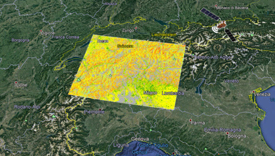
Figure 1.
Footprint of the ascending (in red) and descending (in blue) SAR images over the Alpine arc. The 30m Copernicus DEM is used as the background image.
Figure 1.
Footprint of the ascending (in red) and descending (in blue) SAR images over the Alpine arc. The 30m Copernicus DEM is used as the background image.

Figure 2.
Workflow of the developed semi-automatic methodology. Ri_05minus contains Rindex values lower than 0.5, i.e., those pixels where the influence of topography is the highest. CLC_05plus contains Rindex values higher than 0.5, i.e., those pixels where the influence of land cover is higher than the topography. CLC_Slomask contains pixel in flat areas where the MP detection is influenced only by the land cover. These intermediate products are explained more in detail in Section 3.2.

Figure 3.
Graph builder made in SNAP for processing each SAR image.

Figure 4.
Block chain of the Rindex map model builder developed in ArcGIS. The input data are in dark blue, processes in orange, optional processes in yellow, optional inputs in purple, results of the intermediate process in green, additional parameter in light blue and final output in red. The “P” indicates a required input parameter. Inputs: DEM, digital elevation model; SAR-derived Layover & Shadow mask, mask with pixel values indicating the presence of geometrical effects as output of the graph builder of Figure 3; SAR-derived Local Incidence Angle, per pixel estimation of the local incidence angle; AoI, area of interest. Intermediate outputs: Slope_map, raster file with slope angle per pixel; Aspect_map, raster file with the direction of slope per pixel; Sh/Lh mask, binary raster (1 = no geometric effects, 0 = shadow/layover areas); Flat_area, mask with pixels with null or very low slope values. Final output: Ri_m, Rindex map for the whole image; Ri_m_AoI, Rindex for the area of interest.

Figure 5.
Block chain of the probability of MPD_m developed in ArcGIS and derived by the combination of the Ri_m and the CLC. Input data and output location are in dark blue, processes in orange, optional processes yellow, optional inputs in purple, results of the intermediate process in green, fields of the feature to rasterize in light blue and final output in red. “P” indicates a required input parameter. Inputs: CLC_0m_r, CLC 0 mask (raster) according to Table 2; CLC_05m_r, CLC 05 mask (raster) according to Table 2; workplace, save and storage directory. Intermediate outputs: CLC_0m_AoI and CLC_05m_AoI, CLC masks derived according to Table 2 for the area of interest; DEM_AoI, digital elevation model for the area of interest; Ri_0m, Ri_m which contains the class of CLC unfavorable for the MP detection (CLC_0m); CLC_05minus, CLC_05plus & CLC_Slomask, see the caption of Figure 2. Final output: MPD_m, measurement points detection map.

Figure 6.
Rindex map of the entire test area in ascending (a) and descending (c) orbits and close-ups for ascending (b) and descending (d) tracks.
Figure 6.
Rindex map of the entire test area in ascending (a) and descending (c) orbits and close-ups for ascending (b) and descending (d) tracks.

Figure 7.
Probability of MP detection map of the entire test area in ascending (a) and descending (c) orbits and close ups for ascending (b) and descending (d) tracks.
Figure 7.
Probability of MP detection map of the entire test area in ascending (a) and descending (c) orbits and close ups for ascending (b) and descending (d) tracks.

Figure 8.
Analysis of the percentage of pixels affected by topography and landcover effect of each frame, in both ascending and descending track.
Figure 8.
Analysis of the percentage of pixels affected by topography and landcover effect of each frame, in both ascending and descending track.

Figure 9.
Density ratio calculated for the derived MPD_m over Valle d’Aosta Region.


Table 1.
Rindex map (Ri_m) classification.
| Ri ≤ 0 | Shadow/Layover/Flat Area |
| 0 < Ri < 0.25 | High impact of terrain geometry |
| 0.25 < Ri < 0.5 | Medium impact of terrain geometry |
| 0.5 < Ri < 1 | Low impact of terrain geometry |
Table 2.
Conversion of the CLC classes in values for its classification and use in the probability MP detection tool. Values are referred to a MTInSAR processing identifying both persistent and distributed scatterers.
Table 2.
Conversion of the CLC classes in values for its classification and use in the probability MP detection tool. Values are referred to a MTInSAR processing identifying both persistent and distributed scatterers.
| CLC Code | CLC Class Description | Value | CLC Code | CLC Class Description | Value |
|---|---|---|---|---|---|
| 0mask | 05mask | ||||
| 131 | Mineral extraction sites | 0 | 111 | Continuous urban fabric | 1 |
| 133 | Construction sites | 0 | 112 | Discontinuous urban fabric | 1 |
| 213 | Rice fields | 0 | 121 | Industrial or commercial units | 1 |
| 222 | Fruit trees and berry plantations | 0 | 122 | Road and rail networks and associated land | 0.75 |
| 223 | Olive groves | 0 | 123 | Port areas | 1 |
| 311 | Broad-leaved forest | 0 | 124 | Airports | 1 |
| 312 | Coniferous forest | 0 | 132 | Dump sites | 0.5 |
| 313 | Mixed forest | 0 | 141 | Green urban areas | 0.5 |
| 335 | Glaciers and perpetual snow | 0 | 142 | Sport and leisure facilities | 0.75 |
| 411 | Inland marshes | 0 | 211 | Non-irrigated arable land | 0.5 |
| 412 | Peat bogs | 0 | 212 | Permanently irrigated land | 0.5 |
| 421 | Salt marshes | 0 | 221 | Vineyards | 0.5 |
| 422 | Salines | 0 | 241 | Annual crops associated with permanent crops | 0.5 |
| 423 | Intertidal flats | 0 | 242 | Complex cultivation patterns | 0.5 |
| 511 | Water courses | 0 | 243 | Land principally occupied by agriculture, with areas of natural vegetation | 0.5 |
| 512 | Water bodies | 0 | 244 | Agro-forestry areas | 0.5 |
| 521 | Coastal lagoons | 0 | 321 | Natural grasslands | 0.5 |
| 522 | Estuaries | 0 | 322 | Moors and heathland | 0.5 |
| 523 | Sea and ocean | 0 | 323 | Sclerophyllous vegetation | 0.5 |
| 324 | Transitional woodland-shrub | 0.5 | |||
| 331 | Beaches, dunes, sands | 0.75 | |||
| 332 | Bare rocks | 1 | |||
| 333 | Sparsely vegetated areas | 0.75 | |||
| 334 | Burnt areas | 0.75 | |||
Table 3.
Probability of MP detection map (MPD_m) classification.
| MPD ≤ 0 | Very Low Probability of MP Detection |
| 0 < MPD < 0.25 | Low probability of MP detection |
| 0.25 < MPD < 0.5 | Medium probability of MP detection |
| 0.5 < MPD < 0.75 | High probability of MP detection |
| 0.75 < MPD < 1 | Very high probability of MP detection |
Publisher’s Note: MDPI stays neutral with regard to jurisdictional claims in published maps and institutional affiliations. |
© 2021 by the authors. Licensee MDPI, Basel, Switzerland. This article is an open access article distributed under the terms and conditions of the Creative Commons Attribution (CC BY) license (https://creativecommons.org/licenses/by/4.0/).
Share and Cite
MDPI and ACS Style
Del Soldato, M.; Solari, L.; Novellino, A.; Monserrat, O.; Raspini, F. A New Set of Tools for the Generation of InSAR Visibility Maps over Wide Areas. Geosciences 2021, 11, 229. https://doi.org/10.3390/geosciences11060229
AMA Style
Del Soldato M, Solari L, Novellino A, Monserrat O, Raspini F. A New Set of Tools for the Generation of InSAR Visibility Maps over Wide Areas. Geosciences. 2021; 11(6):229. https://doi.org/10.3390/geosciences11060229
Chicago/Turabian StyleDel Soldato, Matteo, Lorenzo Solari, Alessandro Novellino, Oriol Monserrat, and Federico Raspini. 2021. "A New Set of Tools for the Generation of InSAR Visibility Maps over Wide Areas" Geosciences 11, no. 6: 229. https://doi.org/10.3390/geosciences11060229
Note that from the first issue of 2016, this journal uses article numbers instead of page numbers. See further details here.