Yield Erosion Sediment (YES): A PyQGIS Plug-In for the Sediments Production Calculation Based on the Erosion Potential Method


 , ,
, , 
Abstract
:1. Introduction
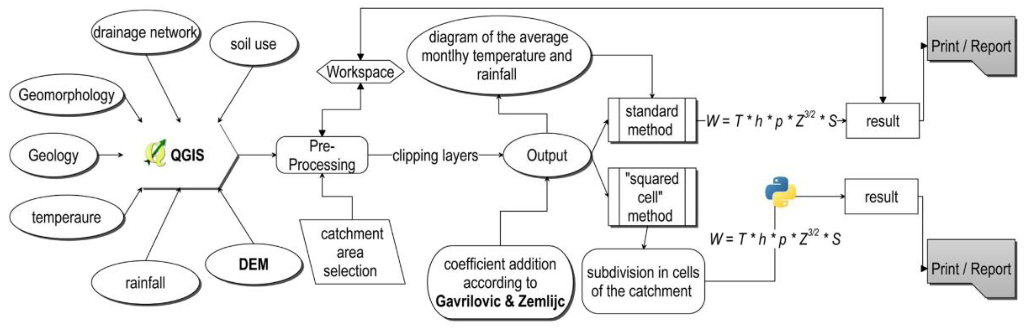
2. Methodology
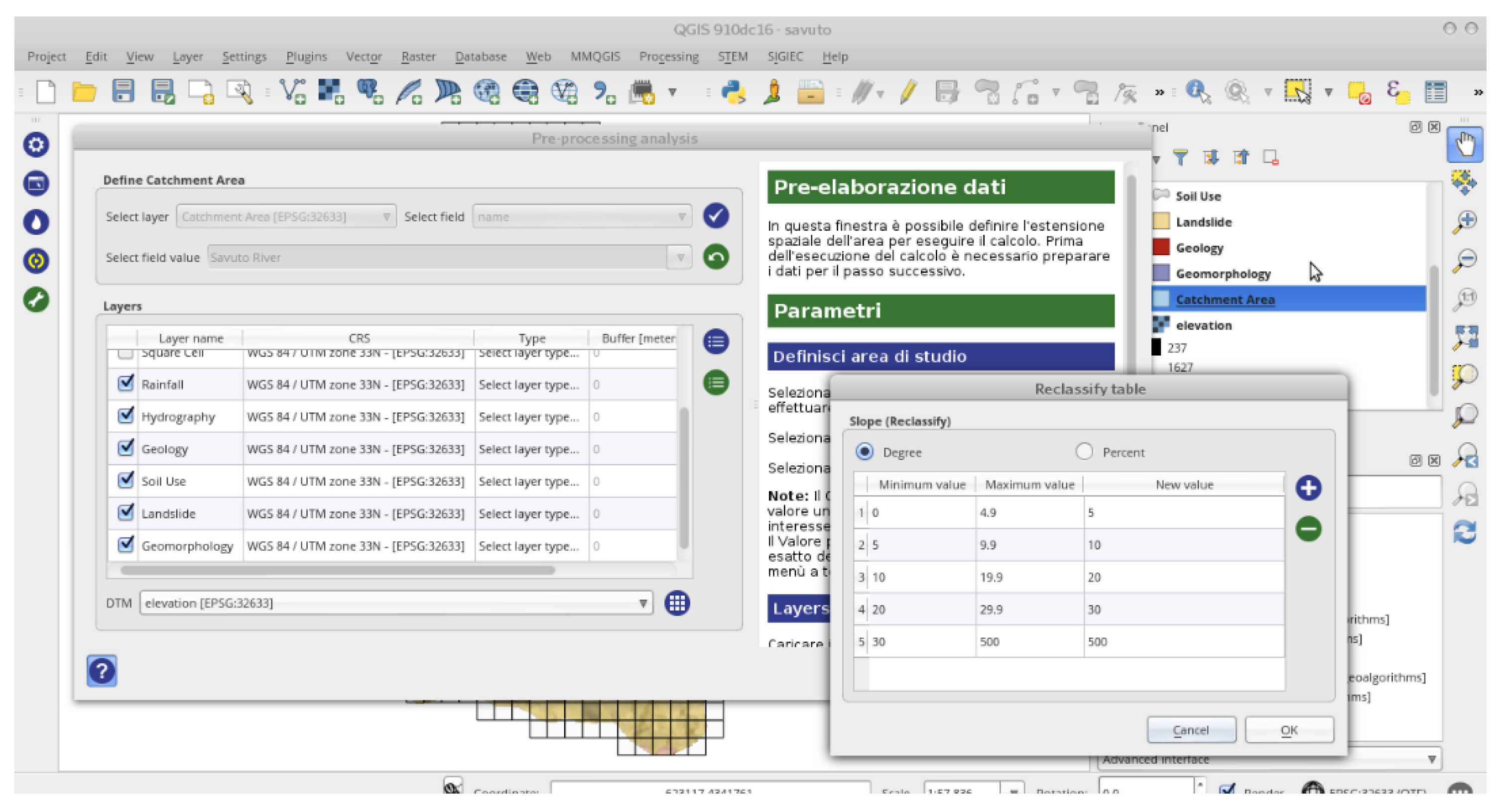
2.1. Stage 1—Preprocessing
- loading layers needed for the geoprocessing analysis as the Digital Elevation Model (DEM) (in ASCII or GeoTIFF formats), geological map, soil use map, drainage network, thermo-pluviometric values or maps, landslides map;
- spatial selection of the catchment area;
- selection of loaded layers for the following operations, e.g., clipping and buffering of the input vector layer, clipping of the Digital Elevation Model and reclassify for the analysis of slope data (using the desired slope classes). At the end of stage 1 all the necessary layers (with the coordinate system selected by the user) are ready for the EPM application.
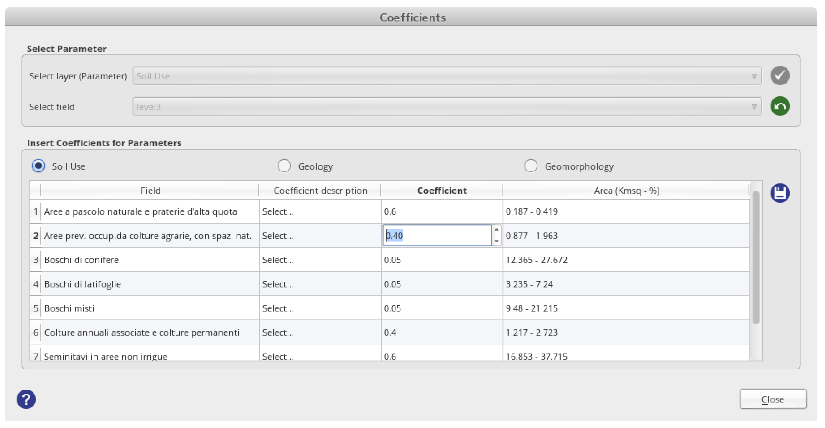
2.2. Stage 2—Selection of the Gavrilović Coefficients
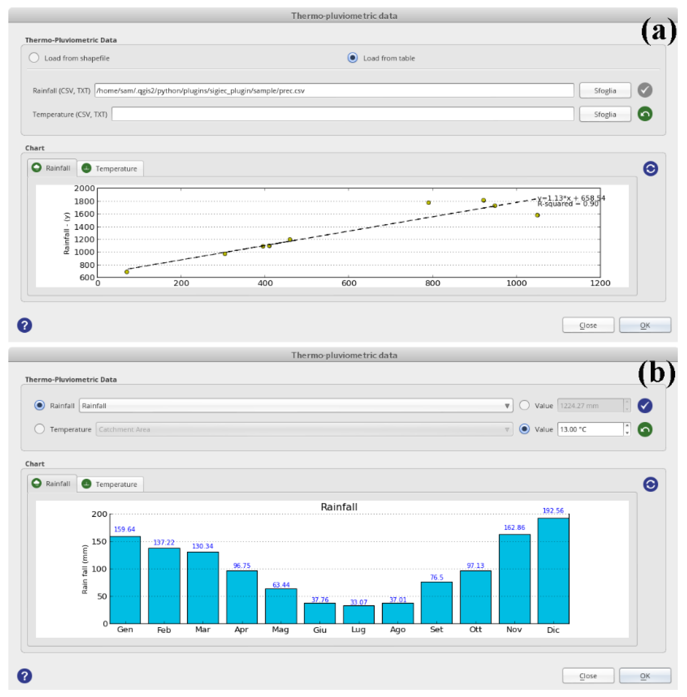
2.3. Stage 3—Thermopluviometric Data
2.4. Stage 4—Final Calculation
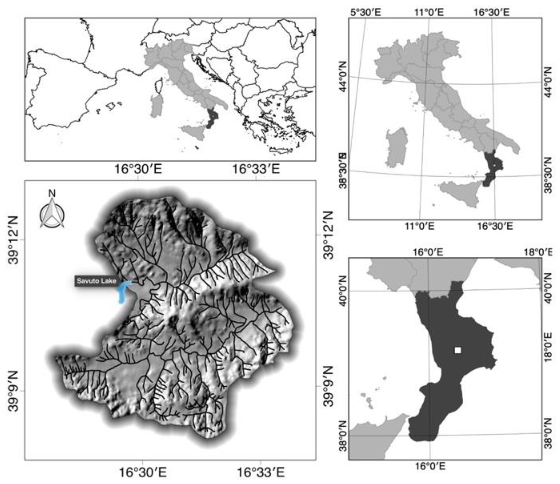
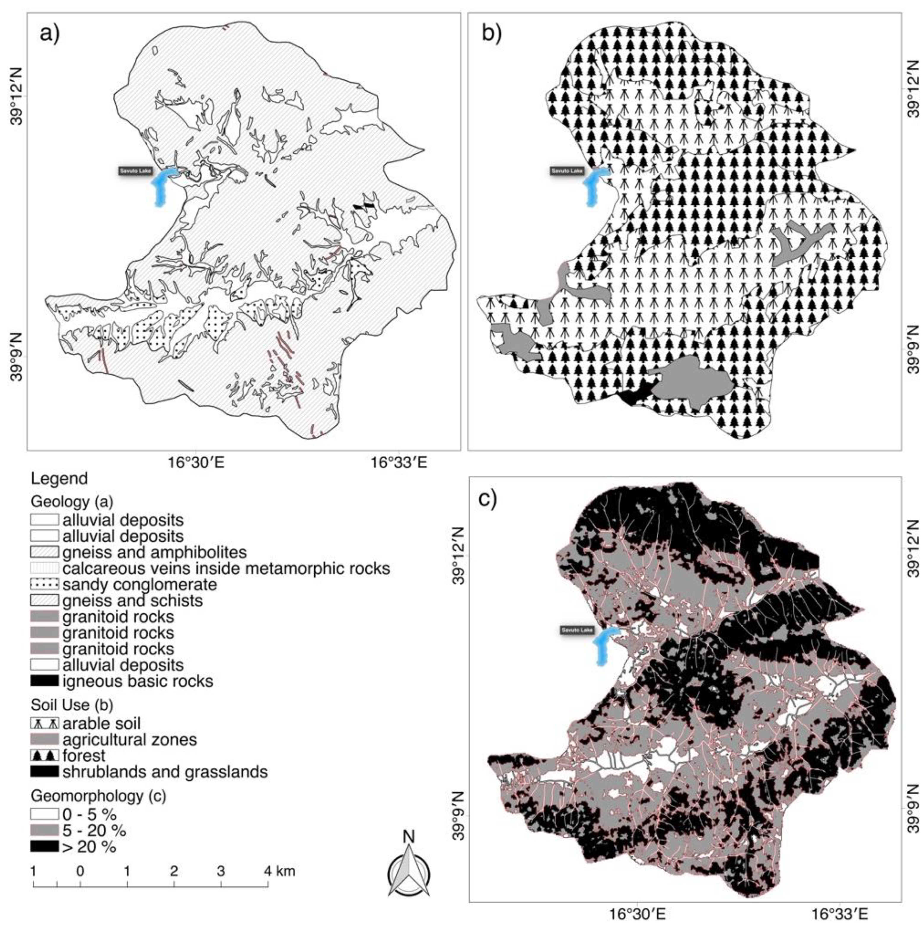
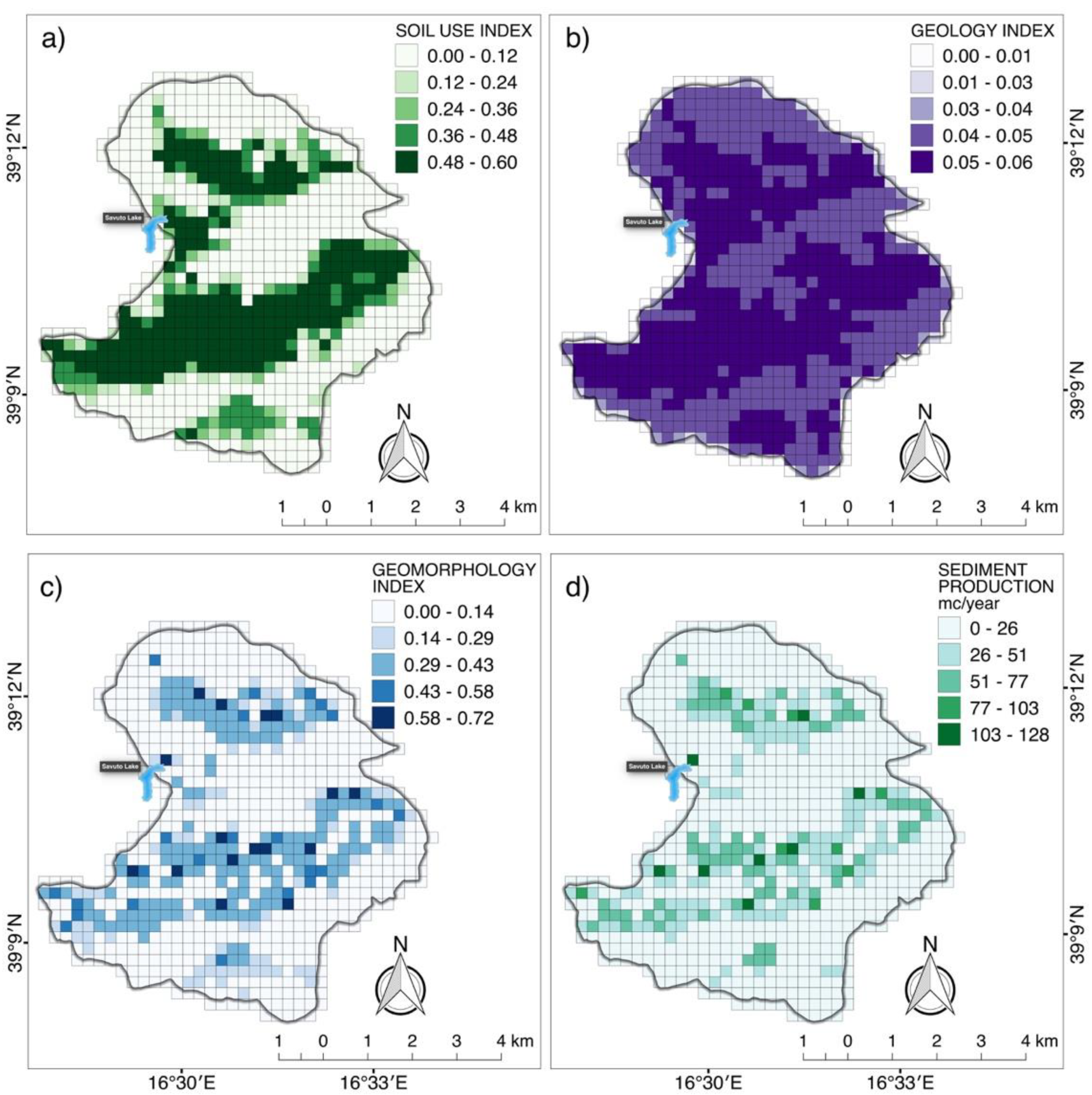
3. Test Application to the Savuto Lake Catchment
4. Discussion
5. Final Remarks
Author Contributions
Funding
Acknowledgments
Conflicts of Interest
References
- Poesen, J.W.; Hooke, J.M. Erosion, flooding and channel management in Mediterranean environments of southern Europe. Prog. Phys. Geogr. 1997, 21, 157–199. [Google Scholar] [CrossRef]
- Vanmaercke, M.; Zenebe, A.; Poesen, J.; Nyssen, J.; Verstraeten, G.; Deckers, J. Sediment dynamics and the role of flash floods in sediment export from medium-sized catchments: A case study from the semi-arid tropical highlands in northern Ethiopia. J. Soil Sediments 2010, 10, 611–627. [Google Scholar] [CrossRef] [Green Version]
- Rago, V.; Chiaravalloti, F.; Chiodo, G.; Gabriele, S.; Lupiano, V.; Nicastro, R.; Pellegrino, A.D.; Procopio, A.; Siviglia, S.; Terranova, O.G.; et al. Geomorphic effects caused by heavy rainfall in southern Calabria (Italy) on 30 October–1 November 2015. J. Maps 2017, 13, 836–843. [Google Scholar] [CrossRef] [Green Version]
- Edward, J.A. The Human influence on the Mediterranean coast over the last 200 years: A brief appraisal from a geomorphological perspective. Géomorphologie 2014, 20, 219–226. [Google Scholar]
- Bonora, N.; Immordino, F.; Schiavi, C.; Simeoni, U.; Valpreda, E. Interaction between Catchment Basin Management and Coastal Evolution (Southern Italy). J. Coast. Res. 2002, 36, 81–88. [Google Scholar] [CrossRef]
- Greco, A.; Furci, D.; Sbrana, F.; Dominici, R. SIGIEC application: An integrated system for management of coastal erosion. Rend. Online Soc. Geol. Ital. 2016, 38, 51–54. [Google Scholar] [CrossRef]
- Rinaldi, M.; Simoncini, C.; Gay, H. Scientific design strategy for promoting sustainable sediment management: The case of the magra river (central-northern Italy). River Res. Appl. 2009, 25, 607–625. [Google Scholar] [CrossRef]
- Eisazadeh, L.; Sokouti, R.; Homaee, M.; Pazira, E. Comparison of empirical models to estimate soil erosion and sediment yield in micro catchments. Eurasian J. Soil Sci. 2012, 1, 28–33. [Google Scholar]
- De Vente, J.; Poesen, J. Predicting soil erosion and sediment yield at the basin scale: Scale issues and semi-quantitative models. Earth-Sci. Rev. 2005, 71, 95–125. [Google Scholar] [CrossRef]
- Gavrilovic, S. Méthode de la Classification des Bassins Torrentiels et équations Nouvelles Pour le Calcul des Hautes Eaux et du Debit Solide. Vadoprivreda, Belgrado. 1959. Available online: https://scholar.google.com/scholar?cites=11067799128590128438&as_sdt=2005&sciodt=0,5&hl=it (accessed on 17 August 2020).
- Gavrilovic, S. Bujicni tokovi i erozija (Torrents and erosion). Gradev. Kal. Beogr. (Serb.) 1976. Available online: https://scholar.google.com/scholar?cites=16943375830502631532&as_sdt=2005&sciodt=0,5&hl=it (accessed on 17 August 2020).
- Gavrilovic, Z. The use of an empirical method (Erosion Potential Method) for calculating sediment production and transportation in unstudied or torrential streams. In Proceedings of the International Conference on River Regime, Wallingford, UK, 18–20 May 1988. [Google Scholar]
- Bazzoffi, P. Methods for net erosion measurement in watersheds as a tool for the validation of models in central Italy. In Proceedings of the Workshop on Soil Erosion and Hillslope Hydrology with Emphasis on Higher Magnitude Events, Leuven, Belgium, 27–30 March 1985. [Google Scholar]
- Emmanouloudis, D.A.; Christou, O.P.; Filippidis, E. Quantitative estimation of degradation in the Alikamon river basin using GIS. In Erosion Prediction in Ungauged Basins: Integrating Methods and Techniques; De Boer, D., Froehlich, W., Mizuyama, T., Pietroniro, A., Eds.; IAHS Publication: Wallingford, UK, 2003; Volume 279. [Google Scholar]
- Tazioli, A. Evaluation of erosion in equipped basins, preliminary results of a comparison between the Gavrilovic model and direct measurements of sediment transport. Environ. Geol. 2009, 56, 825–831. [Google Scholar] [CrossRef]
- Milanesi, L.; Pilotti, M.; Clerici, A.; Gavrilovic, Z. Application of an improved version of the erosion potential method in Alpine areas. Ital. J. Eng. Geol. Environ. 2015, 1, 17–30. [Google Scholar]
- Tangestani, M.H. Comparison of EPM and PSIAC models in GIS for erosion and sediment yield assessment in a semi-arid environment: Afzar catchment, Fars Province, Iran. J. Asian Earth Sci. 2006, 27, 585–597. [Google Scholar] [CrossRef]
- Bagherzadeh, A.; Daneshvae, M.R.M. Sediment yield assessment by EPM and PSIAC models using GIS data in semi-arid region. Front. Earth Sci. 2011, 5, 207–216. [Google Scholar] [CrossRef]
- Ghobadi, Y.; Pirasteh, S.; Pradhan, B.; Ahmad, N.B.; Shafri, H.Z.; Sayyad, G.A.; Kabiri, K. Determine of correlation coefficient between EPM and MPSIAC models and generation of erosion maps by GIS techniques in Baghmalek watershed, Khuzestan, Iran. In Proceedings of the 5th Symposium on Advances in Science and Technology SAStech, Mashhad, Iran, 12–14 May 2011; pp. 1–12. [Google Scholar]
- Ghazavi, R.; Vali, A.; Maghami, Y.; Abdi, J.; Sharafi, S. Comparison of EPM, MPSIAC and PESIAC models for estimating sediment and erosion by using GIS (case study: Ghaleh–Ghaph Catchment, Golestan Province). Geogr. Dev. 2012, 10, 30–32. [Google Scholar]
- Tosic, R.; Dragicevic, S. Methodology update for determination of the erosion coefficient. Glas. Srp. Geogr. Društva 2012, 92, 11–26. [Google Scholar] [CrossRef]
- Barmaki, M.; Pazira, E.; Hedayat, N. Investigation of relationships among the environmental factors and water erosion changes using EPM model and GIS. Int. Res. J. Appl. Basic Sci. 2012, 3, 945–949. [Google Scholar]
- Barmaki, M.; Pazira, E.; Esmali, A. Relationships among environmental factors influencing soil erosion using GIS. Eurasian J. Soil Sci. 2012, 1, 40–44. [Google Scholar]
- Dragicevic, N.; Karleuša, B.; Ožanić, N. GIS based monitoring database for Dubračina river catchment area as a tool for mitigation and prevention of flash flood and erosion. In Proceedings of the 13th International Symposium on Water Management and Hydraulic Engineering, Bratislava, Sovakia, 9–12 September 2013; pp. 553–565. [Google Scholar]
- Dragicevic, N.; Karleuša, B.; Ožanić, N. A review of the Gavrilović method (erosion potential method) application. Građevinar 2016, 68, 715. [Google Scholar] [CrossRef]
- Punzo, M.; Cavuoto, G.; Di Fiore, V.; Tarallo, D.; Ludeno, G.; De Rosa, R.; Cianflone, G.; Dominici, R.; Iavarone, M.; Lirer, F.; et al. Application of X-Band Wave Radar for coastal dynamic analysis: Case test of Bagnara Calabra (south Tyrrhenian Sea, Italy). In Proceedings of the IMEKO International Conference on Metrology for the Sea, Napoli, Italy, 11–13 October 2017. [Google Scholar]
- Punzo, M.; Lanciano, C.; Tarallo, D.; Bianco, F.; Cavuoto, G.; De Rosa, R.; Di Fiore, V.; Cianflone, G.; Dominici, R.; Iavarone, M.; et al. Application of X-Band Wave Radar for coastal dynamic analysis: Case test of Bagnara Calabra (south Tyrrhenian Sea, Italy). J. Sens. 2016. [Google Scholar] [CrossRef] [Green Version]
- Zemljic, M. Calcul du Debit Solide–Evaluation de la Vegetation Comme un des Facteurs Antierosifs. In Proceedings of the International Symposium Interpraevent, Villach, Austria, 1971; Available online: http://www.interpraevent.at/palm-cms/upload_files/Publikationen/Tagungsbeitraege/1971_2_359.pdf (accessed on 17 August 2020).
- Vacca, C.; Dominici, R. Preliminary considerations on the application of the Gavrilović method in GIS environment for the calculation of sediment produced by the catchment area of the Stilaro Fiumara (Calabria southeast). Rend. Online Soc. Geol. Ital. 2015, 33, 104–107. [Google Scholar] [CrossRef]
- Auddino, M.; Dominici, R.; Viscomi, A. Evaluation of yield sediment in the Sfalassà Fiumara (southwestern, Calabria) by using Gavrilovic method in GIS environment. Rend. Online Soc. Geol. Ital. 2015, 33, 3–7. [Google Scholar]
- Cianflone, G.; Dominici, R.; Viscomi, A. Potential recharge estimation of the Sibari Plain aquifers (southern Italy) through a new GIS procedure. Geogr. Tech. 2015, 10, 8–18. [Google Scholar]
- Amodio-Morelli, L.; Bonardi, G.; Colonna, V.; Dietrich, D.; Giunta, G.; Ippolito, F.; Liguori, V.; Lorenzoni, S.; Paglionico, A.; Perrone, V.; et al. L’arco Calabro-Peloritano nell’orogene appenninico Maghrebide (The Calabrian-Peloritan Arc in the Apennine-Maghrebide orogen). Mem. Soc. Geol. Ital. 1976, 17, 1–60. [Google Scholar]
- Messina, A.; Russo, S.; Borghi, A.; Colonna, V.; Compagnoni, R.; Caggianelli, A.; Fornelli, A.; Piccarreta, G. Il Massiccio della Sila, Settore settentrionale dell’Arco Calabro-Peloritano (The Sila Massif, northern sector of the Calabrian-Peloritan Arc). Boll. Soc. Geol. Ital. 1994, 113, 539–586. [Google Scholar]
- Scarciglia, F. Weathering and exhumation history of the Sila Massif upland plateaus, southern Italy: A geomorphological and pedological perspective. J. Soils Sediments 2015, 15, 1278–1291. [Google Scholar] [CrossRef]
- Le Pera, E.; Arribas, J.; Critelli, S.; Tortosa, A. The effects of source rocks and chemical weathering on the petrogenesis of siliciclastic sand from the Neto River (Calabria, Italy): Implications for provenance studies. Sedimentology 2001, 48, 357–377. [Google Scholar] [CrossRef]
- Molin, P.; Pazzaglia, F.J.; Dramis, F. Geomorphic expression of active tectonics in a rapidly-deforming forearc, Sila Massif, Calabria, Southern Italy. Am. J. Sci. 2004, 304, 559–589. [Google Scholar] [CrossRef]
- Olivetti, V.; Cyr, A.J.; Molin, P.; Faccenna, C.; Granger, D.E. Uplift history of the Sila Massif, southern Italy, deciphered from cosmogenic 10Be erosion rates and river longitudinal profile analysis. Tectonics 2012, 31, TC3007. [Google Scholar] [CrossRef]
- Cianflone, G.; Tolomei, C.; Brunori, C.A.; Dominici, R. Preliminary study of the surface ground displacements in the Crati Valley (Calabria) by means of InSAR data. Rend. Online Soc. Geol. Ital. 2015, 33, 20–23. [Google Scholar] [CrossRef]
- Cianflone, G.; Tolomei, C.; Brunori, C.A.; Monna, S.; Dominici, R. Landslides and subsidence assessment in the Crati Valley (Southern Italy) using InSAR data. Geoscience 2018, 8, 67. [Google Scholar] [CrossRef] [Green Version]
- Federico, S.; Avolio, E.; Bellecci, C.; Pasqualoni, L. Preliminary results of a 30-year daily rainfall database in southern Italy. Atmos. Res. 2009, 94, 641–651. [Google Scholar] [CrossRef]
- Casmez (Cassa Speciale per il Mezzogiorno). Carta Geologica della Calabria 1:25000. Poligrafica & Cartevalori; Napoli; 1967–1969. Available online: http://geoportale.regione.calabria.it/opendata (accessed on 17 August 2020).
- Rete del Sistema Informativo Nazionale Ambientale. Available online: http://www.sinanet.isprambiente.it/it/sia-ispra/download-mais/corine-land-cover/corine-land-cover-2012/view (accessed on 30 October 2019).
- ABR Regione Calabria. Piano Stralcio di Bacino per l’Assetto Idrogeologico. 2011. Available online: http://old.regione.calabria.it/abr/index.php?option=com_content&task=view&id=364&Itemid=113 (accessed on 30 July 2020).
- MAREGOT. Available online: http://interreg-maritime.eu/web/maregot (accessed on 30 July 2020).
- VEROCOST. Available online: http://verocost.sister.it/ (accessed on 30 July 2020).
- SMORI. Available online: http://www.smori.eu/ (accessed on 30 July 2020).


| Empirical Models | Factors |
|---|---|
| PSIAC | Surface geology; Soil, Climate; Runoff; Topography; Land use; Ground cover; Upland erosion; Channel erosion and sediment transport; |
| FSM | Topography; Vegetation Cover; Gullies; Lithology; Catchment shape; |
| VSD | Vegetation; Surface material; Drainage density; |
| EHU | Relief; Rainfall; Vegetation; Soil; |
| CORINE | Soil erodibility; Rain erosivity; Slope angle; Land cover. |
| FKSM | Slope Rainfall erosivity; soil erodibility; land cover type; Soil disturbance, |
| CSSM | Land use; Ground cover; Topography; Soil erodibility Sediment delivery; Upland contribution; Channel contribution; Future supply; Sediment control; Disturbance period; |
| WSM | Soil type; Vegetation condition; Sign of active soil erosion; Catchment slope; Mean annual rainfall; Catchment area. |
| GLASOD | Water erosion; Wind erosion; Chemical degradation; Physical deterioration; |
| FLORENCE | Catchment area; Digital terrain model; Land use; temperature and rain; hydrographic network; landslide; |
| WATEM-SEDEM | Rainfall erosivity; Soil erodibility; Topography; Crop and management; erosion control practice; |
| SPADS | Vegetation Cover; Topography; Lithology; Rainfall intensity; Gully; Inverse distance from a river stream. |
| USLE | Rainfall erosivity; Soil erodibility; Digital elevation model; Cover management; Support practice |
| RUSLE | Digital elevation model; Rainfall erosivity; Soil erodibility; cover and management factor; the support practice. |
| INRA | Landuse; Soil crustability and soil erodibility (determined by pedotransfer rules from the French soil database); Digital Elevation model; Meteorological data (250 × 250 m) |
| LISEM | Aggregate stability, crop height, cohesion, additional cohesion caused by roots and leaf area index, Manning’s n., percentage vegetation cover, random roughness parallel to slope, random roughness perpendicular to slope, total width of wheeltracks within a pixel, winter-wheat, winter-barley, oats, coleseed and flax. |
| EUROSEM | Runoff based on water balance; Soil detachment based on kinetic energy of rain, unit stream power, the transport capacity deficit, shear strength of the soil and the settling velocity.; |
| WEPP | Runoff based on water balance; Soil detachment based on Slope; Vegetation; Shear stress; Shear strength; Roughness; Organic matter; Root mass. |
| LAPSUS | Digital elevation model; Precipitation; Soil erodibility; Land use related infiltration |
| PESERA | Erodibility based on land use, soil and vegetation cover; digital elevation model; runoff and climate/vegetation soil erosion potential based on gridded data, vegetation cover, water balance and a plant growth model. |
| SLEMSA | Relief; Rainfall; Vegetation; Soil |
| Soil Use (X). | Value |
| Land (loose) denuded | 1.0 |
| Fields cultivated according to the maximum slope | 0.9 |
| Orchards and vineyards without vegetation on the ground | 0.7 |
| Pastures and forests | 0.6 |
| Arable meadows and cultures | 0.4 |
| Forests | 0.05 |
| Soil Resistance (Y) | Value |
| Hard rocks | 0.4 |
| Moderately resistant rocks | 0.8 |
| Crumbly rocks (shales, overconsolidated clays) | 1.15 |
| Little resistant rocks) | 1.55 |
| Loose sediment or not very resistant to erosion | 1.95 |
| Geomorphology () | Value |
| Diffuse erosion (low slope) | 0.15 |
| Diffuse erosion (medium slope) | 0.4 |
| Diffuse erosion (high slope) | 0.65 |
| Linear erosion | 0.85 |
| Landslides | 1.0 |
| Coefficient | Value |
|---|---|
| X (Soil use) | 0.282 |
| Y (Soil resistance) | 0.83 |
| (Geomorphology) | 0.213 |
| Z | 0.15 |
| Catchment average slope (Im) (%) | 17.65 |
| Catchment area (km2) | 44.68 |
| Rainfall (mm) | 1224.27 |
| Temperature (°C) | 15.06 |
| sediment production estimation (Wy) (m3/year) | 21821.6 |
| River Catchments | Region (Country) | Lon, Lat (Catchment Centroid) | Area (km2) | Wy by Standard Method (m3 year−1) | Wy by “Squared Cell” Method (m3 year−1) | Difference (m3 year−1) (%) |
|---|---|---|---|---|---|---|
| Aron | Calabria (Italy) | 15.99, 39.54 | 37.48 | 30,864.03 | 28240.59 | 2623.44 (−8.5%) |
| Sfalassà | Calabria (Italy) | 15.82, 38.24 | 24.03 | 54,769.66 | 49,785.62 | 4984.04 (−9.10%) |
| Cancello | Calabria (Italy) | 16.45, 38.95 | 18.27 | 8,723.38 | 7,938.27 | 785.10 (−9%) |
| Riu Solanas | Sardinia (Italy) | 9.45, 39.17 | 44.03 | 12,623.84 | 11,298.34 | 1325.50 (−10.5%) |
| Esaro (Dam) | Calabria (Italy) | 16.93, 39.64 | 245.48 | 169,030.16 | 153,648.42 | 15,381.74 (−9.1%) |
| Savuto (Dam) | Calabria (Italy) | 16.52, 39.17 | 44.68 | 21,821.60 | 19,639.54 | 2182.17 (−10%) |
© 2020 by the authors. Licensee MDPI, Basel, Switzerland. This article is an open access article distributed under the terms and conditions of the Creative Commons Attribution (CC BY) license (http://creativecommons.org/licenses/by/4.0/).
Share and Cite
Dominici, R.; Larosa, S.; Viscomi, A.; Mao, L.; De Rosa, R.; Cianflone, G. Yield Erosion Sediment (YES): A PyQGIS Plug-In for the Sediments Production Calculation Based on the Erosion Potential Method. Geosciences 2020, 10, 324. https://doi.org/10.3390/geosciences10080324
Dominici R, Larosa S, Viscomi A, Mao L, De Rosa R, Cianflone G. Yield Erosion Sediment (YES): A PyQGIS Plug-In for the Sediments Production Calculation Based on the Erosion Potential Method. Geosciences. 2020; 10(8):324. https://doi.org/10.3390/geosciences10080324
Chicago/Turabian StyleDominici, Rocco, Salvatore Larosa, Antonio Viscomi, Luca Mao, Rosanna De Rosa, and Giuseppe Cianflone. 2020. "Yield Erosion Sediment (YES): A PyQGIS Plug-In for the Sediments Production Calculation Based on the Erosion Potential Method" Geosciences 10, no. 8: 324. https://doi.org/10.3390/geosciences10080324