Simple Summary
World communities are concerned about the impacts of a hotter and drier climate on future agriculture. By examining Australian regional livestock data on sheep, beef cattle, dairy cattle, and pigs, the authors find that livestock production will expand under such conditions. Livestock revenue per farm is expected to increase by more than 47% by 2060 under the UKMO, the GISS, and a high degree of warming CSIRO scenario. The existence of a threshold temperature for these species is not evident.
Abstract
This paper examines the vulnerabilities of major livestock species raised in Australia to climate change using the regional livestock profile of Australia of around 1,400 regions. The number of each species owned, the number of each species sold, and the aggregate livestock revenue across all species are examined. The four major species analyzed are sheep, beef cattle, dairy cattle, and pigs. The analysis also includes livestock products such as wool and milk. These livestock production statistics are regressed against climate, geophysical, market and household characteristics. In contrast to crop studies, the analysis finds that livestock species are resilient to a hotter and more arid climate. Under the CSIRO climate scenario in which temperature increases by 3.4 °C, livestock revenue per farm increases significantly while the number of each species owned increases by large percentages except for dairy cattle. The precipitation reduction by about 8% in 2060 also increases the numbers of livestock species per farm household. Under both UKMO and GISS scenarios, livestock revenue is expected to increase by around 47% while the livestock population increases by large percentage. Livestock management may play a key role in adapting to a hot and arid climate in Australia. However, critical values of the climatic variables for the species analyzed in this paper are not obvious from the regional data.
1. Introduction
The earth has been warming, according to the Intergovernmental Panel on Climate Change (IPCC), due in large part to anthropogenic activities such as fossil fuel uses, agricultural emissions and land use changes [1]. The impacts of climate change are expected to vary geographically with the largest impacts felt in low latitude developing countries where agriculture plays a key economic role [2-5]. Climate change is likely inevitable and thus adaptation is becoming a widely discussed policy option [6]. Recently, economic research has started to examine possible adaptation options [7-12] and this area of work will continue to grow given the inevitable need for adaptation to climate change [6,13-15].
Empirical studies indicate that livestock management may be quite resilient against global warming and arid conditions due to climate change. For example, Seo and Mendelsohn found African farmers adapted by choosing goats and sheep more frequently when climate becomes hotter [7]. In Latin America, findings indicate farmers rely on sheep more than beef cattle under hotter climates [8]. Also, integrated crop and livestock management is found to be more common under hotter conditions than farms specializing in only crops [9,12] with integrated farms predicted to suffer only half the damage in land values from the 21st century climate change [10]. In the U.S., findings are that hotter conditions cause animal breeds to be adapted toward more of a Brahman influence [16] when stocking rates fall and land shifts from cropland to pasture [17]. This economically based literature has an animal science parallel in which the climate drivers leading to changes in animal breed selection are debated [18]. Animal scientists have also long investigated relationships between climate factors and animal production [19-21]. Finally, animal science and more general climate literature indicate that adaptive capacity of different livestock species to climate stress varies and that management options are available to facilitate adaptation [22,23]. Thus, in heavy livestock producing countries, climate change adaptation may be needed and alternatives are available. Policy makers, farmers and others may wish to carefully examine livestock sensitivity and adaptation in low-latitude countries which are both heavily dependent on livestock management and argued to be highly vulnerable to climate change [24-26].
Australia is a country that relies heavily on livestock for domestic consumption and exports. In such a setting, a closer examination of the interplay between climate, climate change and livestock is an important issue but one that is often left out of policy discussions [27]. The mix of livestock species and breeds that would better adapt to hotter conditions due to genetic components or other reasons is one of the fundamental adaptation research questions for scientists [18]. Research on livestock adaptation would provide important information paralleling findings on the crop side where crops are reported to be differentially vulnerable to temperature increases and rainfall reduction [2,28-30].
This paper examines the ways livestock management in Australia varies with climate as an input to identifying adaptation strategies and their effectiveness. Regional livestock data are obtained from the Australian Bureau of Statistics (ABS) [31], the Australian Bureau of Agricultural and Resource Economics (ABARE) [32] with climate data drawn from the Climate Research Unit [1,33]. Soils data are from Zobler's World File for Global Climate Modeling [34,35] and vegetation and land cover information is from the Matthews' Vegetation and Land Use Data [36].
These data are examined to see climate influences on livestock populations and revenues from sales of sheep, beef cattle, dairy cattle, and pigs. Regressions were run against climatic variables, along with geophysical (soil and geographic), market and household characteristic factors. The availability of feed from crop production is also examined. Marginal impacts of temperature and precipitation are examined by livestock species. In turn the effects of projected 2060 climate scenarios from the Australian Commonwealth Scientific and Industrial Research Organization (CSIRO) [1,37] and the IPCC A2 scenarios from the GISS (Goddard Institute for Spatial Studies) [38] and UKMO (United Kingdom Meteorology Office) [39] models. Specifically, the GISS-ER model and HadGEM1 model of the UKMO documented in the IPCC Data Distribution Center are examined.
This paper proceeds as follows. A brief description of the theory and methodology used to examine the variation of livestock revenue and species across climate zones is provided in the next section. The following section presents a detailed description of the data set. In the subsequent sections, empirical estimation results and the consequences of the projected 2060 climate scenarios are analyzed. The paper ends with discussions and conclusion.
2. Methods
To examine the effects of climate on livestock species choice and revenue, a statistical estimation approach is used with climate and non-climate signals to which a farmer responds controlled as explanatory variables. Classical economic profit maximizing is assumed. Suppose a farmer chooses a livestock species mix from a set of available animal species to maximize profit considering the given climate, geophysical, market and household factors. Then, the choices of species across the landscape would capture the best outcomes as climate and other conditions are varied [40].
More formally, let πj be the profit from species j. Then, a livestock producer's problem can be written as follows:
The maximization determines the choices of species and the optimal mix of inputs and outputs. The maximized profit can then be written as a function of exogenous variables as follows:
Among the factors that determine profit for livestock species j, climate (E) is the primary concern of this analysis; G represents a great diversity of geophysical conditions involving soils and geography across Australia; M captures economic market conditions such as access to livestock export ports as well as urban markets; H reflects household characteristics such as whether the farm has complementary feed from grain productions or number of vehicles owned.
The impact of a change in climate on species j can be measured as the difference in the estimated profits under two climate conditions. That is, if climate is changed from E1 to E2, then the impact is measured as follows:
3. Description of Data
Livestock ownership and revenue data were drawn from the 2006 regional profile of Australia compiled by the Australian Bureau of Statistics (ABS) for around 1,400 local areas [31]. These data contain the reported numbers of beef cattle, dairy cattle, sheep/lambs, and pigs at each locality, and also contain data on revenue from livestock slaughter and livestock products such as wool and milk.
Livestock sale data came from the Australian Bureau of Agricultural and Resource Economics [32]. That Bureau reported data for the years 1990 to 2009 for 34 sub-regions in terms of average statistics based on surveys conducted using random sampling. The data set also reported livestock product volume and included information on socio-economic variables such as age of the manager and off-farm labor hours.
Climate data in terms of monthly average temperature and precipitation were drawn from the Climate Research Unit. These data are at the scale of 10 arc minute, based on more than 27,000 global weather stations [33]. In the Southern Hemisphere, data were aggregated into summer (December, January, and February) and winter (June, July, and August) observations. Using the ArcView toolbox, the centroid of each locality in the ABS data was calculated and the climate data were interpolated to that centroid using a shortest distance method.
Soil data were from the Zobler's World File for Global Climate Modeling [34]. The data set reports a dominant soil for each grid cell of the globe. Most frequently found Australian soils are Acrisols, Cambisols, Ferralsols, Phaeozems, Lithosols, Luvisols, Nitosols, Podzols, Arenosols, Regosols, Solonetz, Andosols, Vertisols, Planosols, Xerosols, Yermosols, and Solonchaks. Many local areas are also near a water body such as the Murray Darling Basin or along the coasts.
Socio-economic variables were obtained from the ABS regional profile of Australia [31] consisting of information on human population density and distribution as well as household characteristics such as vehicle ownership, racial composition, female ratio, and building construction at the local level.
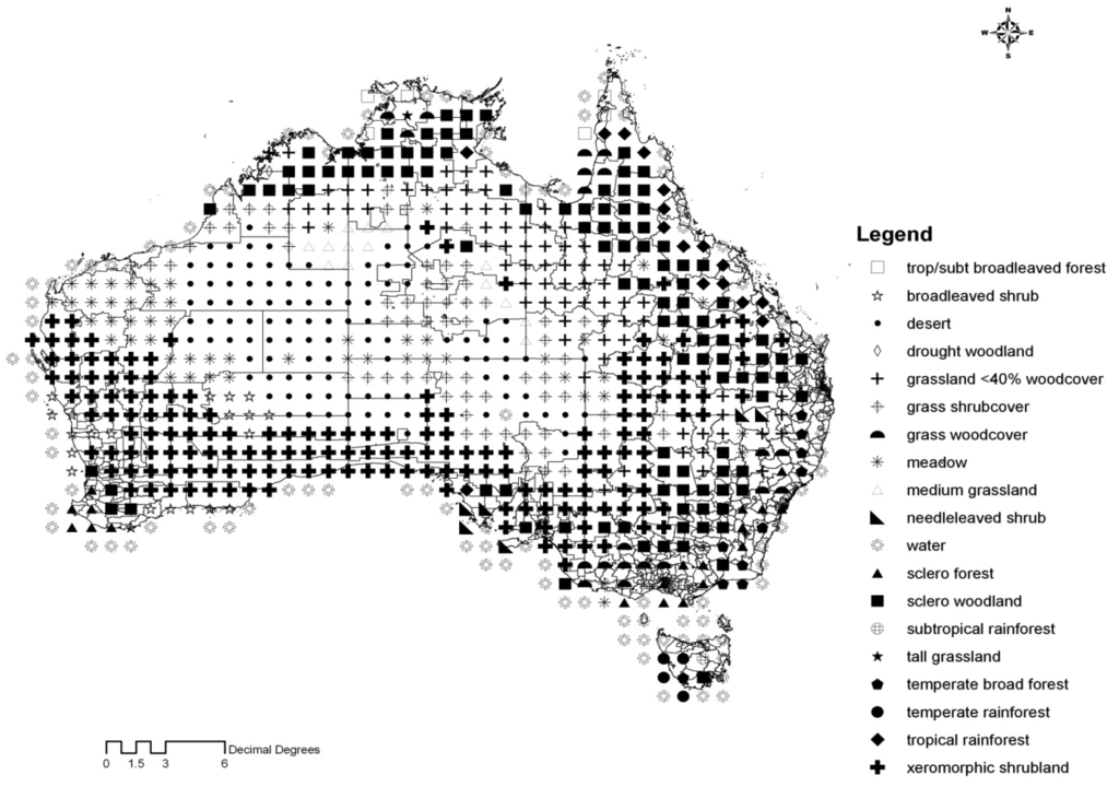
Finally, major vegetation and land cover data were drawn from the Global Land Use and Vegetation data set [36]. As shown in Figure 1, Australia contains diverse ecological systems and land covers [42]. Along the eastern coast of Australia are mostly temperate broadleaved forests. Adjacent to the forests are sclerophyllous woodlands. Further inlands are xeromorphic shrublands. Central parts of Australia are occupied by grasslands and deserts. Southern Australia is mostly made up of xeromorphic shrublands. Western Australia is a mixture of forests, woodlands, and shrublands in the south, and a combination of shrublands and meadow in the north. Northern parts are drought affected deciduous woodlands, sclerophyllous forests, and grasslands.
4. Empirical Results
State and Territory level descriptive statistics computed across the local areas with reported livestock populations are summarized in Table 1. Summer temperatures range from 15 °C in Tasmania (TAS) to 28 °C in the Northern Territory (NT). Winter temperature is as low as 5 °C in the Australian Capital Territory (ACT). The driest State is Western Australia (WA) in the summer and NT in the winter. Xerosols are dominant soils in South Australia (SA) while Planosols are most common in WA and NT. On average, ACT is located in higher altitudes. The proportion of the population that are females is lower than 0.5, especially in NT and ACT. The number of passenger vehicles per 1,000 people is larger in New South Wales (NSW) and Victoria (VIC). New building approvals are larger in VIC and WA.

Average livestock sales per farm during the 1990 to 2009 period summarized by species/product and sub-region are discussed in the next section [43]. Averaged over the 20 year period, beef cattle sales are largest in the Barkly Tablelands in the NT with 3,273 cattle per year per farm. The Kimberly region of WA sells around 1,700 cattle per year. The smallest sale is recorded at the wheat belt in WA with 7 per farm. Sheep sale is largest in the Far West in NSW with 1,284 head per farm and in Central and South Wheat Belt in WA with 1,339 head per farm. Total sale of wool is well matched with the sale of sheep, but is second largest in North Pastoral region of South Australia (SA). There is limited sale of sheep or wool in the regions of NT and WA where cattle sales are greater.
To examine how climate influences the variation in beef cattle, dairy cattle, sheep, and pig populations, the number of animals by species is regressed against seasonal climatic variables, physical, socio-economic factors and regional household characteristics with the results presented in Table 2, Table 3, Table 4, and Table 5. For each species, we run two regressions with and without household characteristic variables. The dependent variable is the log of the number of animals by species per 1,000 rural people in the area. Results for the sheep regression are presented in Table 2. Focusing on the full model, summer temperature and precipitation turn out to be highly significant with P-values less than 0.01. The model R-sq is high at 0.72. The positive quadratic term of summer temperature indicates a U-shaped response. That is, when summer temperature rises beyond a certain point, the number of sheep owned increases.
The results indicate that soils and geographic variables are relevant factors in raising sheep. The sheep number owned is higher in an area which is farther from the coast. The number increases at higher altitudes. Fewer sheep are raised on Acrisols, Cambisols, and Xerosols soils while more sheep are raised in Lithosols and Vertisols. Socio-economic variables are also significant. When the female ratio in the human population rises, there are fewer sheep raised. The number of passenger vehicles and building approvals is negatively associated with sheep ownership. But, when there are more pension receivers, sheep ownership is larger.
The regression results for beef cattle are presented in Table 3. Again, summer temperature turns out to be critical with a positive quadratic term indicating a U-shaped response. The number of beef cattle increases in larger towns and at high elevations. Fewer beef cattle are raised on Xerosols whereas more beef cattle are raised on Ferralsols, Podzols, and Vertisols. Fewer beef cattle are raised in a district with a higher unemployment rate or more building approvals. When the number of pension receivers increases, the number of beef cattle owned also increases. The results that more sheep and beef cattle are raised in the areas with lower building approvals or more pension receivers may reflect the fact that pension receivers more often live in the rural areas and new building constructions are lower there.
In Table 4, dairy cattle exhibit a hill-shaped temperature response contrary to the findings for sheep and beef cattle, but only winter temperature terms, linear and quadratic, are significant at 5%. Larger numbers of dairy cattle are raised on Ferralsols, Phaeozems, and Luvisols. The regression reveals a strong socio-economic influence. Fewer dairy cattle are raised in high unemployment zones. An increase in passenger vehicles or building approvals decreases the number of dairy cattle while an increase in pension receivers increases it. An increase in female ratio in the human population decreases the ownership of dairy cattle substantially. Female ratio is higher in major cities. Dairy cattle are only raised in half the towns that raise beef cattle. This is probably due to the higher water requirements involved with raising dairy cattle, e.g., through the Murray Darling basin. This is also confirmed in the positive estimate for the “water body” variable which is only significant in the case of dairy cattle. The Adj Rsq of the model is also low.
Results for the number of pigs are presented in Table 5. Parameter estimates are significant for precipitation and temperature variables. It shows a hill-shaped response with summer temperature. Fewer pigs are owned in Regosols, Vertisols, and Xerosols. The higher the elevation, the more pigs are raised. The smaller the town, the more pigs are raised. Most socio-economic variables are not significant. More building approvals mean fewer pigs are raised. More pension receivers imply more pigs are raised.
A regression on the aggregate livestock sector revenue, which is defined as the total summed revenue from the sales of all livestock species and products, is shown in Table 6. It also includes milk and wool productions. The Adj Rsq is 0.46. The linear terms of winter temperature and summer precipitation are significant at 1%. Livestock revenue is higher in many soils except Xerosols. Revenue is also higher in high elevations or inland locations. The higher the unemployment rate, the lower the livestock revenue. The larger the number of building approvals, the lower the livestock revenue. An area with more pension receivers has higher livestock revenue.
5. Impact and Sensitivity Analysis
Marginal impacts of a change in the climate variables are calculated based on the estimated regressions and are shown in Table 7. Based on the full models, if temperature increases by 1 °C, beef cattle and pigs increase with an elasticity of +0.36 and +0.54 respectively. On the other hand, sheep and dairy cattle decrease with an elasticity of −0.16 and −0.34 respectively. On aggregate, livestock revenue increases with an elasticity of +0.27. The results can be contrasted with crop studies which find that in hotter areas some crops are severely harmed by a warmer climate [28,30]. This implies that Australian farmers may increase livestock over crops when temperature becomes hotter, as has been found elsewhere [9,10,17].
When precipitation increases by 1%, beef cattle, sheep, and pigs decline in numbers with an elasticity of −0.07, −0.49, and −0.67 respectively. Dairy cattle increase but only slightly. Thus, wetter conditions decrease livestock populations likely by increasing cropped area as found in [9,10,17]. Furthermore, livestock revenue falls with an elasticity of −0.09. Again, the results can be contrasted with crop studies which report that crops generally benefit from increased rainfall [2,28]. An alternative interpretation is that slightly less rainfall causes more livestock production. Sheep and cattle are also raised more often in drier zones of Africa and Latin America [7,8].
An alternative specification without socio-economic factors leads to similar but slightly different results, as shown in the middle panel of Table 7. When temperature increases, marginal elasticities are slightly smaller with an exception of sheep. When precipitation increases, the elasticity of beef cattle turns positive, an indication of a mis-specification due to omitted household variables. Therefore, the full model should be preferred to the model without social variables.
In the above analyses, the impact of climate change on crops and the availability of feed were not explicitly considered. A hotter and drier climate is beneficial for livestock since it alters the landscape from forests or croplands to pasture suitable for livestock but at the same time, can lead to reduced feed available from grain production. To explicitly test the impact of reduced feed on livestock production, additional regressions were run and are presented in Table 8 by adding a variable for feed availability. The size of the land used for grain production is used as a proxy for feed availability. The regressions for the five dependent variables indicate that feed availability/cropland use does affect the number of each species owned and the aggregate livestock revenue, i.e., the estimates are significant at 5%. Alternatively, livestock management may have increased the demand for crops to be used for feed. Interestingly, feed availability decreases the number of dairy cattle owned while it increases the numbers of other species owned. This implies that dairy cattle are substitutes for grains while beef cattle, sheep, and pigs are complementary goods. That is, if climate conditions are the same, a municipality with a larger grain land raises larger numbers of beef cattle, sheep, and pigs because of feed availability, but not dairy cattle.
Marginal elasticities based on the model including feed availability/cropland use are presented at the bottom panel of Table 7 using the feed availability model in Table 8. There are no significant changes in the elasticities except that precipitation elasticity turned negative in the case of dairy cattle. First, these results imply that the indirect impact of climate change on feed availability is implicitly captured in the full models of Table 2,Table 3,Table 4,Table 5 and Table 6. But the changed sign of dairy cattle elasticity may indicate that dairy cattle and crops often compete for resources such as land and water.
Lastly, Australia is one of the largest livestock exporters in the world with Japan, China, South Korea, Indonesia, and the US being the largest importers of Australian livestock. Over two thirds of Australian agriculture is exported. Agriculture accounts for about 20% of Australian merchandise exports, more than half of which comes from livestock [44]. Given the nature of the cross-sectional data set employed, Australian farmers across different climate zones faced export conditions similar to the survey year 2006. Across the landscape, however, access to export market participation varies a great deal. In our regressions in the previous section, they are captured by the distance to coasts and number of passenger vehicles owned. Estimates in Table 2,Table 3,Table 4,Table 5 and Table 6 indicate that distance to coastal markets and the number of passenger vehicles are not a major factor, i.e., their estimates are not significant. Good road and transportation systems across the country developed for livestock exports, e.g., Australian Livestock Transporters Association (ALTA) and Livestock and Bulk Carriers Association (LBCA), may have eliminated the obstacles of transportation to access ports.
A simple analysis in Table 9 compares the sales of beef cattle, sheep, and wool per farm business in 1990 with those in 2009 using the ABARE surveys since 1990. It is notable that beef cattle sales have increased dramatically over this time period in the Northern Territory and Western Australia, the regions which are climatically unfriendly for humans, due primarily to the improved road and transportation systems. Therefore, improved access to export markets in the future will likely further increase production of livestock in Australia in these remote regions. What will happen to foreign demand is less clear. If climate is shifted globally, overseas demands for Australian livestock may fall due to increased productions in the US, Africa, and Latin America [9,10,17] but foreign demands may increase elsewhere such as Middle East, South Asia, and northern Europe. Decreased international demands will result in increased transportation fees to remote zones since transporters are supposed to charge more, which will lead to decreased productions in these remote grasslands. In our regressions, these effects are partially captured by the coefficients in the distance to coasts.
6. Climate Scenarios
The long term impacts of climate change on the livestock sector are examined in this section based on the estimated parameters of the full models. This exercise is meant to single out the sole impacts of climate scenarios on the livestock sector keeping all other factors fixed. Therefore, this exercise excludes the external influences of technological changes, population growth, environmental attitudes, and economic development.
Three General Circulation Model scenarios (GCMs) used in the recent IPCC report [1] were used in this examination. Specifically, the A2 scenarios from the GISS ER model (Goddard Institute for Spatial Studies) [38] and HadGEM1 model of the UKMO (United Kingdom Meteorology Office) [39] were used. These scenarios were obtained from the IPCC's Data Distribution Center. In addition, a high degree warming scenario from the Commonwealth Scientific and Industrial Research Organization (CSIRO) was examined [37]. By 2060, the CSIRO scenario predicts a 3.4 °C increase in annual mean temperature and an 8% reduction in annual precipitation [42]. As shown in Table 10, both the GISS and the UKMO scenarios forecast temperature increases of around 2 °C in both summer and winter seasons for the time period between 2040 and 2070. The UKMO scenario predicts a drier climate in both summer and winter while the GISS scenario predicts an increase in summer rainfall by around 10%.
In Table 11, the impacts of these climate scenarios are calculated for the four livestock species and livestock revenue. The top and middle panels of Table 11 show the impacts of the high degree warming CSIRO scenario using the full models. When temperature increases by as much as 3.4 °C, sheep and beef cattle show substantial increases. Sheep increase by 57%, beef cattle by 240%, and pigs by 9%. The number of sheep increases by a large percentage due to U-shaped temperature response functions (Table 7). On the other hand, dairy cattle fall by 10%. Aggregated over all species, livestock revenue increases by around 62%.
When precipitation decreases by 8%, it is notable that all the species benefit from the drier conditions. Sheep and pig populations increase by around 30%. The increases in beef cattle and dairy cattle are modest. Aggregated across all the species as well as various products such as milk and wool, livestock revenue also increases but merely by 0.06%. The impacts of the changes in both temperature and precipitation result in a population change of +82% for sheep, +242% for beef cattle, −9.5% for dairy cattle, and +40% for pigs, along with a +62% increase in livestock revenue.
In the bottom panel of the Table 11, simulation results from the GISS and UKMO scenarios are presented. Across the four species, the increases are far larger under the UKMO scenario, i.e., a hotter and drier scenario. Sheep increase by 122%, beef cattle by 211%, dairy cattle by 29%, and pigs by 72%. A wetter summer predicted by the GISS scenario decreases the desirability of these species. For example, the expected sheep increase is only 22% while dairy cattle decrease by 2%. Again, dairy cattle may compete against crops under milder and wetter conditions. The overall impact on livestock revenue is not different, however, with around 47% increase in revenue in both cases.
What might be the reasons for the increased numbers and revenue from livestock under hotter and drier conditions? Animals may have adaptive capacity to heat and other environmental stress [21]. Numerous management adjustments may also play a significant role in protecting the animals [22,23]. For example, famers might pursue genetic adaptation such as use of a more heat tolerant Brahman cattle breed [18] or substitute livestock for crops when climate becomes hot and arid [9,10,17].
6. Discussion
This paper examines the vulnerabilities of livestock species populations and revenue in Australia to climate change. The analysis was based on 2006 livestock population and sales data of the regional livestock profile in around 1,400 local areas. Four major species were examined: beef cattle, dairy cattle, sheep, and pigs. Livestock products such as wool and milk are also analyzed.
The results show that when temperature increases marginally, beef cattle and pig populations increase. On the other hand, dairy cattle and sheep decrease. Furthermore, across all the species, total livestock revenue per farm increases. When precipitation falls marginally, beef cattle, sheep, and pig populations increase but dairy cattle decrease. Across all species, livestock revenue increases, implying that a drier climate will benefit livestock managers except for those with dairy cattle.
Under projected long term climate change scenarios, the results indicate four species raised would increase by large percentages. Under the hotter and drier UKMO HadGEM1 scenario, sheep would increase by 122%, beef cattle by 211%, dairy cattle by 29%, and pigs by 71%. If, on the other hand, the GISS scenario comes to pass, sheep would increase only by 22% due to a projected wetter summer. In both scenarios, livestock revenue is expected to increase by +47% by around 2060. Under the higher degree warming scenario by the CSIRO, these changes become even larger.
In interpreting the results, several qualifications need to be added. These findings seem to contradict the scientific studies of cattle which indicated decreased weight growth and conception of cattle due to increased heat stress, but are in line with the vegetation studies which predict increased grasslands for livestock [45]. Livestock species may face threshold climate values which are not evident from the regional data used in this study as the temperature could rise beyond the ranges in the data [21]. Secondly, this paper does not determine, due to data limitations, whether alternative breeds of cattle or sheep would be abandoned or favored due to their vulnerability or resilience [18]. Third, goats and chickens were omitted from the analysis as data were not available, so they are conspicuously missing in the analysis. Fourth, whether increased pasture under the hot and arid conditions means low quality of grass and lessened productivity is not fully addressed by the results in this research except to the extent that current climate variations and livestock activities contain such variation. However, the impacts of the changes of a more extreme nature, outside of the range of historic variation, such as 50% drop in rainfall cannot be answered from this research. Fifth, the research does not incorporate the possibility that altered livestock populations may lead to increased greenhouse gas emissions, and increased cost under the carbon tax regime [46]. However, cases exist where methane emissions from livestock can be reduced substantially with little cost by feed management and dietary additives, which may become needed for Australian producers [47]. Finally, there are no available household level micro data that allow examination of household climate adaptation choices including feed purchase alternatives, so this is omitted.
7. Conclusion
The findings in this paper show livestock management is likely to be more resilient under a hotter and drier world than are crops. In climate zones like Australia, findings have shown that major crops may be highly vulnerable to climate change [28,30]. The finding that livestock species can be raised successfully under more arid conditions may deserve special attention by farm mangers and policy makers as they weigh adaptation possibilities. This is particularly true in Australia, which has vast areas of grasslands nationwide except for the forested areas along the eastern coasts. This research finds that climate change favors cattle and sheep although this merits local examination in terms of the suitability of species and breeds. The underlying driver of these results involves land use change, lowered disease incidence and intrinsically lower vulnerability relative to crops [45,48-51]. Given that climate change will unfold over the next 100 years, a wise adaptation portfolio which includes the livestock sector is certainly called for.
Acknowledgements
Authors thank the Agricultural and Resource Economics seminar participants at the University of Sydney for their helpful comments. We are particularly grateful to Irene Hoffmann at the Food and Agriculture Organization (FAO) who read and provided thoughtful comments on several rounds of drafts. The manuscript has benefited from the three anonymous reviewers' comments.
References and Notes
- Intergovernmental Panel on Climate Change (IPCC). Climate Change 2007: The Physical Science Basis; Fourth Assessment Report; Cambridge University Press: Cambridge, UK, 2007. [Google Scholar]
- Reilly, J.; Baethgen, W.; Chege, F.E.; Van De Geijn, S.C.; Erda, L.; Iglesias, A.; Kenny, G.; Patterson, D.; Rogasik, J.; Rotter, R.; Rosenzweig, C.; Sombroek, W.; Westbrook, J.; Bachelet, D.; Brklacich, M.; Dammgen, U.; Howden, M.; Joyce, R.J.V.; Lingren, P.D.; Schmmelpfenning, D.; Singh, U.; Sirotenko, O.; Wheaton, E. Agriculture in a Changing Climate: Impacts and Adaptations. In Climate Change 1995: Impacts, Adaptations, and Mitigation of Climate Change: Scientific-Technical Analyses; Watson, R.T., Zinyowera, M.C., Moss, R.H., Dokken, D.J., Eds.; Cambridge University Press: Cambridge, UK, 1996; pp. 427–468. [Google Scholar]
- Nordhaus, W.; Boyer, J. Warming the World: Economic Models of Global Warming; MIT Press: Cambridge, MA, USA, 2000. [Google Scholar]
- Gitay, H.; Brwon, S.; Easterling, W.; Jallow, B. Ecosystems and Their Goods and Services. In Climate Change 2001: Impacts, Adaptations, and Vulnerabilities; Cambridge University Press: Cambridge, UK, 2001; pp. 237–342. [Google Scholar]
- Parry, M.L.; Canziani, O.F.; Palutikof, J.P.; Van Der Linden, P.J.; Hanson, C.E. Climate Change 2007: Impacts, Adaptations, and Vulnerability; Cambridge University Press: Cambridge, UK, 2007. [Google Scholar]
- Rose, S.; McCarl, B. Greenhouse Gas Emissions, Stabilization and the Inevitability of Adaptation: Challenges for Agriculture. Choices 2008, 23, 15–18. [Google Scholar]
- Seo, S.N.; Mendelsohn, R. Measuring Impacts and Adaptations to Climate Change: A Structural Ricardian Model of African Livestock Management. Agr. Econ. 2008, 38, 151–165. [Google Scholar]
- Seo, S.N.; McCarl, B.; Mendelsohn, R. From Beef Cattle to Sheep under Global Warming? An Analysis of Adaptation by Livestock Species Choice in South America. Ecol. Econ. 2010, 69, 2486–2494. [Google Scholar]
- Seo, S.N. Is an Integrated Farm More Resilient Against Climate Change? A Micro-Econometric Analysis of Portfolio Diversification in African Agriculture. Food Pol. 2010, 35, 32–40. [Google Scholar]
- Seo, S.N. A Microeconometric Analysis of Adapting Portfolios to Climate Change: Adoption of Agricultural Systems in Latin America. Appl. Econ. Perspect. Pol. 2010, 32, 489–514. [Google Scholar]
- Seo, S.N. An Analysis of Public Adaptation to Climate Change Using Agricultural Water Schemes in South America. Ecol. Econ. 2011, 70, 825–834. [Google Scholar]
- Seo, S.N. A Geographically Scaled Analysis of Adaptation with Spatial Models Using Agricultural Systems in Africa. J. Agr. Sci. 2011, 149, 437–449. [Google Scholar]
- Smith, J. Setting Priorities for Adaptation to Climate Change. Global Environ. Change 1997, 7, 251–264. [Google Scholar]
- Smit, B.; Burton, I.; Klein, R.J.T.; Wandel, J. An Anatomy of Adaptation to Climate Change and Variability. Clim. Change 2000, 45, 223–251. [Google Scholar]
- Tol, R.S.J.; Yohe, G.W. The Weakest Link Hypothesis for Adaptive Capacity: An Empirical Test. Global Environ. Change 2007, 17, 218–227. [Google Scholar]
- Zhang, Y.W.; Hagerman, A.D.; McCarl, B.A. How Climate Factors Influenced the Spatial Allocation and Returns to Texas Cattle Breeds. Proceedings of the 2011 Annual Meetings of the Agricultural and Applied Economics Association, Pittsburgh, PA, USA, 24–26 July 2011.
- Mu, J.H.; McCarl, B.A. Adaptation to Climate Change: Land Use and Livestock Management. Proceedings of the 2011 Annual Meetings of the Southern Agricultural Economics Association, Corpus Christi, TX, USA, 5–8 February 2011.
- Hoffmann, I. Climate Change and the Characterization, Breeding and Conservation of Animal Genetic Resources. Anim. Genet. 2010, 41, 32–46. [Google Scholar]
- Johnson, H.D. The Response of Animals to Heat. Meteorol. Monograph 1965, 6, 109–122. [Google Scholar]
- Johnson, H.D. Aspects of Animal Biometeorology in the Past and Future. Int. J. Biometeorol. 1997, 40, 16–18. [Google Scholar]
- Hahn, G.L. Dynamic Responses of Cattle to Thermal Heat Loads. J. Anim. Sci. 1999, 77, 1–11. [Google Scholar]
- Hahn, G.L. Housing and Management to Reduce Climate Impacts on Livestock. J. Anim. Sci. 1981, 52, 175–186. [Google Scholar]
- Mader, T.L. Environmental Stress in Confined Beef Cattle. J. Anim. Sci. 2003, 81, 110–119. [Google Scholar]
- Magrin, G.; Garcia, C.G.; Choque, D.C.; Gimenez, J.C.; Moreno, A.R.; Nagy, G.J.; Carlos, N.; Villamizar, A. Latin America. In Climate Change 2007: Impacts, Adaptation, and Vulnerability; Parry, M.L., Canziani, O.F., Palutikof, J.P., van der Linden, P.J., Hanson, C.E., Eds.; Cambridge University Press: Cambridge, UK; pp. 581–615.
- Boko, M.; Niang, I.; Nyong, A.; Vogel, C.; Githeko, A.; Medany, M.; Osman-Elasha, B.; Tabo, R.; Yanda, R. Africa in Climate Change 2007: Impacts, Adaptation and Vulnerability; Parry, M.L., Canziani, O.F., Palutikof, J.P., van der Linden, P.J., Hanson, C.E., Eds.; Cambridge University Press: Cambridge, UK; pp. 433–467.
- Agriculture for Development; World Development Report; The World Bank: Washington, DC, USA, 2008.
- Garnaut, R. Climate Change and the Australian Agricultural and Resource Industries. Aust. J. Agr. Resour. Econ. 2010, 54, 9–25. [Google Scholar]
- Adams, R.; Rosenzweig, C.; Peart, R.M.; Ritchie, J.T.; McCarl, B.A.; Glyer, J.D.; Curry, R.B.; Jones, J.W.; Boote, K.J.; Allen, L.H. Global Climate Change and US Agriculture. Nature 1990, 345, 219–224. [Google Scholar]
- Butt, T.A.; McCarl, B.A.; Angerer, J.; Dyke, P.T.; Stuth, J.W. The Economic and Food Security Implications of Climate Change in Mali. Clim. Change 2005, 68, 355–378. [Google Scholar]
- Schlenker, W.; Roberts, M. Nonlinear Temperature Effects Indicate Severe Damages to Crop Yields under Climate Change. Proc. Nat. Acad. Sci. USA 2009, 106, 15594–15598. [Google Scholar]
- Australian Bureau of Statistics. National Regional Profile, 2005–2009; The Australian Government: Canberra, Australia, 2010. [Google Scholar]
- Australian Bureau of Agriculture and Resource Economics (ABARE). ABARE Farm Surveys. Available online: http://www.abare.gov.au/publications_html/surveys/surveys/surveys.html (accessed on 3 July 2010).
- New, M.; Lister, D.; Hulme, M.; Makin, I. A High-resolution Data Set of Surface Climate over Global Land Areas. Clim. Res. 2002, 21, 1–25. [Google Scholar]
- Zobler, L. A World Soil File for Global Climate Modeling; NASA Technical Memorandum 87802; NASA Goddard Institute for Space Studies (GISS): New York, NY, USA, 1986. [Google Scholar]
- Food and Agriculture Organization. The Digital Soil Map of the World (DSMW); FAO: Rome, Italy, 2003. Available online: http://www.fao.org/AG/agl/agll/dsmw.stm (accessed on 9 March 2004).
- Matthews, E. Global Vegetation and Land Use: New High-resolution Data Bases for Climate Studies. J. Clim. Appl. Meteorol. 1983, 22, 474–487. [Google Scholar]
- Commonwealth Scientific Industrial Research Organization (CSIRO). OzClim-Climate Change Scenario Generator, 2010. Available online: http://www.csiro.au/ozclim/home.do (accessed on 7 March 2011).
- Schmidt, G.A.; Ruedy, R.; Hansen, J.E.; Aleinov, I.; Bell, N.; Bauer, M.; Bauer, S.; Cairns, B.; Canuto, V.; Cheng, Y.; et al. Present Day Atmospheric Simulations Using GISS ModelE: Comparison to in-situ, satellite and reanalysis data. J. Clim. 2005, 19, 153–192. [Google Scholar]
- Gordon, C.; Cooper, C.; Senior, C.A.; Banks, H.T.; Gregory, J.M.; Johns, T.C.; Mitchell, J.F.B.; Wood, R.A. The Simulation of SST, Sea Ice Extents and Ocean Heat Transports in a Version of the Hadley Centre Coupled Model without Flux Adjustments. Clim. Dynam. 2000, 16, 147–168. [Google Scholar]
- Mendelsohn, R.; Nordhaus, W.; Shaw, D. The Impact of Global Warming on Agriculture: A Ricardian Analysis. Am. Econ. Rev. 1994, 84, 753–771. [Google Scholar]
- Heckman, J. Sample Selection Bias as a Specification Error. Econometrica 1979, 47, 153–162. [Google Scholar]
- Seo, S.N. The Impacts of Climate Change on Australia and New Zealand: A Gross Cell Product Analysis by Land Cover. Aust. J. Agri. Resour. Econ. 2011, 55, 220–238. [Google Scholar]
- The statistics are based on the household surveys conducted and compiled annually by the Australian Bureau of Agricultural and Resource Economics and Sciences.
- Agriculture and the WTO; Department of Foreign Affairs and Trade: Canberra, ACT, Australia, 2011.
- Donald, G.E.; Edirisinghe, A.; Hill, M.J.; Sneddon, J.N.; Hyder, M.; Warren, B.; Wheaton, G.A.; Craig, R. A Semi-Automated Approach to Continuous Assessment of Pasture Growth Rate and Feed on Offer in South West Western Australia. In West Australian Forum Merino Research and Innovation Proceedings; Merinotech: Kojonup, Australia, 2000; pp. 20–25. [Google Scholar]
- Nordhaus, W. The Architecture of Climate Economics: Designing a Global Agreement on Global Warming. Bull. Atom. Sci. 2011, 67, 9–18. [Google Scholar]
- Global Mitigation of Non-CO2 Greenhouse Gases; US Environmental Protection Agency: Washington, DC, USA, 2006. Available online: http://www.epa.gov/climatechange/economics/downloads/GlobalMitigationFullReport.pdf (accessed on 18 October 2011).
- Sankaran, M.; Hanan, N.P.; Scholes, R.J.; Ratnam, J.; Augustine, D.J.; Cade, B.S.; Gignoux, J.; Higgins, S.I.; Le Roux, X.; Ludwig, F.; Ardo, J.; Banyikwa, F.; Brown, A.; Bucini, G.; Caylor, K.K.; Coughenour, M.B.; Diouf, A.; Ekaya, W.; Feral, C.j.; February, E.C.; Frost, P.G.H.; Hiernaux, P.; Hrabar, H.; Metzger, K.L.; Prins, H.H.T.; Ringrose, S.; Sea, W.; Tews, J.; Worden, J.; Zambatis, N. Determinants of Woody Cover in African Savannas. Nature 2005, 438, 846–849. [Google Scholar]
- White, N.; Sutherst, R.W.; Hall, N.; Whish-Wilson, P. The Vulnerability of the Australian Beef Industry to Impacts of the Cattle Tick (Boophilus microplus) under Climate Change. Clim. Change 2003, 61, 157–190. [Google Scholar]
- Communicating Climate Change: Climate Change Impacts on Pest Animals and Weeds; Meat and Livestock Association (MLA): North Sydney, Australia, 2008.
- Foreign Animal Diseases: The Greybook; College of Veterinary Medicine, University of Georgia, 2007. Available online: http://www.vet.uga.edu/vpp/grey_book02 (accessed on 11 March 2009).
© 2011 by the authors; licensee MDPI, Basel, Switzerland. This article is an open access article distributed under the terms and conditions of the Creative Commons Attribution license (http://creativecommons.org/licenses/by/3.0/).