1. Introduction
To realize high-resolution tasks, analog actuators are generally employed [
1,
2]. These actuators are able to realize continuous motions within their working stroke limits. In literature, many analog actuators have been developed to realize, as well as planar [
1,
3], rotary [
4,
5,
6] or combined motions [
7]. Sensory components need to be integrated for the control of these actuators in order to ensure high resolution positioning or precise trajectories [
7,
8]. The control laws are generally complex, according to the high-performance levels needed. Moreover in highly integrated or compact mechatronic systems, the integration of sensory components is sometimes difficult or even impossible. For these reasons, actuators based on a digital principle are one of the interesting alternatives.
Digital (or binary) actuators consist of a mobile part able to switch between repeatable and well known discrete positions. The main advantage of digital actuators is that an internal energy holding of the mobile part in discrete position is provided so that external energy supply (pulses) is only needed to switch the mobile part between the discrete positions [
9]. It provides several interests. Firstly, this pulse mode control ensures a low energy consumption because there is no need of energy to hold the mobile part in discrete position [
10,
11]. The control can also lead to a very simple open loop binary control [
12,
13] because the digital actuation ensures highly repeatable and accurate discrete positions which do not need external measurement systems [
14]. The integration of these actuators in mechanical or mechatronic systems is then easy. In addition, digital outputs of a data acquisition board can be used to control digital actuators instead of analog outputs needed for analog actuators, which decreases the total cost of the system. Another advantage of this pulse mode is the reduction of the Joule effect due to the short duration of the control pulse [
15].
However due to their digital principle, digital actuators present some limitations and requirements. The main limitation is relative to their discrete stroke fixed at the manufacturing step. In standard functioning, the mobile part of digital actuators can indeed not stop in an intermediate position located between two discrete positions. This limitation can be overcome since variable strokes can been achieved using an assembly of several digital actuators [
12]. Otherwise, a crucial requirement to ensure high-precision tasks is the high manufacturing quality required for digital actuators (surface, tolerance,
etc.) because the influence of manufacturing errors cannot be compensated by a closed loop control.
Two functions are needed to perform digital actuation: the driving function, to switch the mobile part between the discrete positions, and the holding function, to hold the mobile part in discrete position. In literature, the driving function is generally obtained via electrostatic [
16], thermal [
17,
18] electromagnetic [
19,
20] or piezoelectric [
21] physical effects. For the holding function, three commonly used methods are employed, such as magnetic effect [
19,
20], compliant mechanisms [
18,
22], and position locking actuators [
23].
Due to their simplicity, digital actuators are used in various types of applications which can be classified into two categories. The first one regroups devices composed of a single digital actuator as electrical [
11,
16], optical [
24,
25], and fluidic [
26,
27] switches. The second category includes devices where several actuators are integrated so that complex tasks can be realized by combination of elementary actions. Switches arrays [
27], tactile display devices [
28], digital-to-analog converters [
29], digital robots [
12,
30], and distributed conveyance devices [
31,
32] are some examples of these applications.
In this work, a high-precision electromagnetic digital actuator is presented. The electromagnetic principle has been chosen because it is well adapted for digital actuation. As a matter of fact, it can manage both holding and switching functions: a magnetic holding force can be easily obtained using the magnetic property of the mobile permanent magnet while the driving force is obtained electromagnetically (Lorentz force). Compared to the literature, the main originality of the presented digital actuator is that the mobile part can perform displacements along two orthogonal directions without an assembly of two 1D actuators [
33]. This configuration reduces the assembly errors, thus enhancing the precision of the actuator and improving its compactness.
A first version of this actuator was previously developed and tested along one axis only [
20]. In the presented paper, an optimized and more compact version of the actuator is presented. In a first part, the principle and the architecture of this new version is described. An analytical model of the actuator is used to characterize the energy consumption and the maximal displaceable mass. Then an experimental prototype is presented and tested. Comparisons between experimental and simulated results are carried out. The positioning repeatability errors have been measured to characterize the digital behavior of the actuator and its high-precision property. Finally, an example of application which takes advantage of the two orthogonal displacement directions and the high-precision positioning is described and experimentally tested.
2. Principle
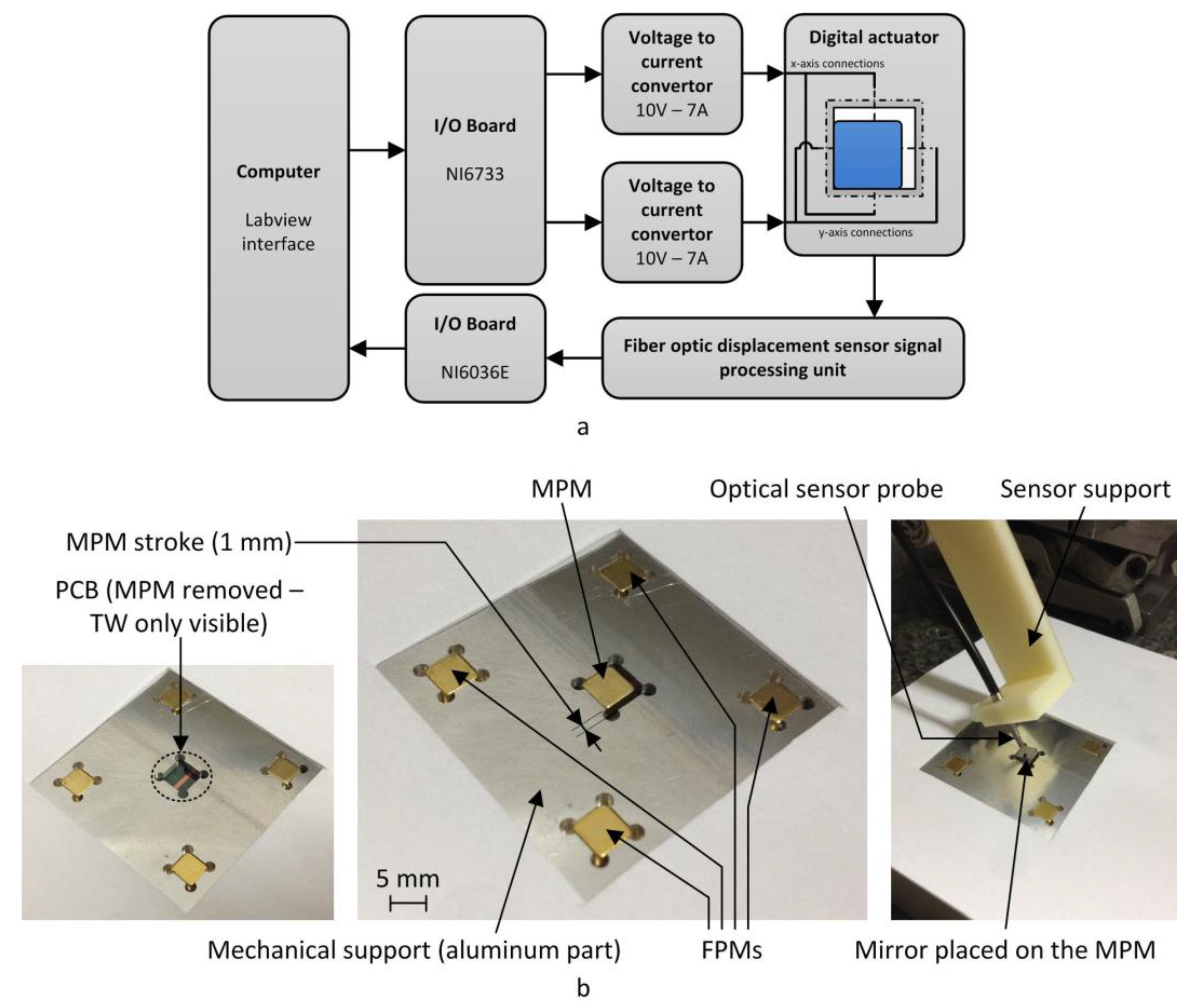
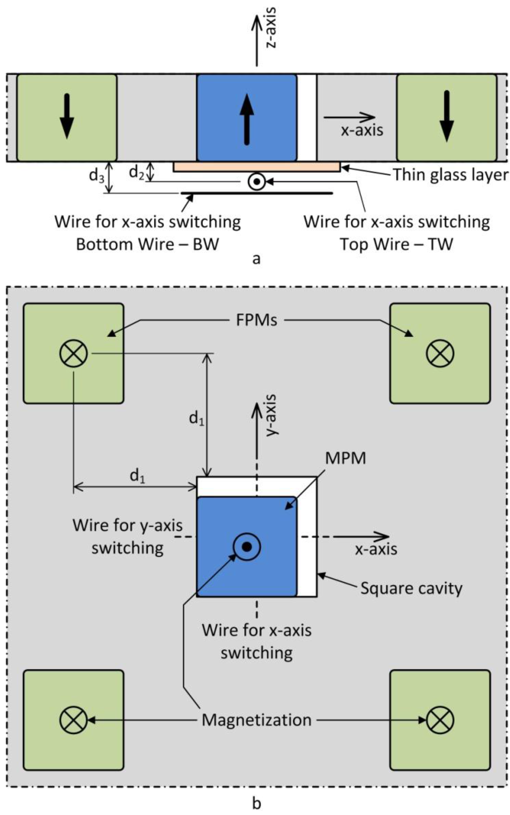
The presented actuator is composed of a mobile part, which is a parallelepiped mobile permanent magnet (MPM), and a fixed part which regroups a square cavity, four fixed permanent magnets (FPMs) and two orthogonal wires (
Figure 1). The MPM is placed in a square cavity and can reach its four corners which correspond to the four discrete positions of the actuator. The gap between the MPM and the square cavity characterizes the actuator stroke. Four FPMs, with a magnetization orientated in the opposite direction as compared to the MPM, are placed near each corner so that a magnetic attraction force is exerted on the MPM in discrete position. This magnetic force ensures the holding function which characterizes the positioning repeatability of the MPM in discrete position then the high precision property of the presented actuator. The switching function of the MPM between the discrete positions is obtained using two electrical wires placed below the cavity. When a current passes through a wire, a Lorentz force is generated between the MPM and the wire. Since the wire is fixed, the MPM moves thanks to this force. In order to get an electrical insulation between the two wires, one wire is printed on the top side of a double side printed circuit board (PCB) and second one on the bottom side. The wire placed closed to the MPM (distance
d2 in
Figure 1) is called top wire (TW) and is used to switch the MPM along
x-axis. The second wire placed far away from the MPM (distance
d3 in
Figure 1) is called bottom wire (BW) and is used to switch the MPM along
y-axis. In order to minimize the difference of the Lorentz force generated by the two wires on the MPM, the thickness of the PCB has been chosen as small as possible (200 µm). Moreover, a thin glass layer of 170 µm thickness is placed between MPM and the PCB to avoid electrical contact between the TW and the MPM and provide a flat surface. The geometrical, magnetic, and electromagnetic properties of the actuator are given in
Table 1.
In
Figure 1, the MPM is located in the discrete position (–
xMPM; –
yMPM). If a switch along the +
x direction is desired, a driving current should be injected through the “wire for
x-axis switching” (TW) in the –
y direction. This current will generate a Lorentz force on the TW in the –
x direction due to the orientation of MPM magnetic flux density in the +
z direction (left hand rule). Since the TW is fixed, an opposite force in the +
x direction is exerted on the MPM which switches to reach the discrete position (+
xMPM ; –
yMPM). During this switch, the holding force in the –
y direction can be increased using a holding current through the “wire for
y-axis switching” (BW) in the –
x direction. This increase in the holding force can be interesting to reduce the influence of disruptions during the MPM switch and to increase the positioning precision of the MPM in discrete position.
Figure 1.
Principle of the four discrete positions actuator: (a) side view, and (b) top view.
Figure 1.
Principle of the four discrete positions actuator: (a) side view, and (b) top view.
The high-precision property of the actuator is characterized by the magnetic holding force generated by the FPMs on the MPM. An increase of the magnetic holding force ensures a higher positioning precision of the MPM in discrete positions even in the presence of high disturbances; nevertheless, the energy consumption needed to switch from one position to another one will also increase. For the presented actuator, a compromise between the high-precision digital behavior and the minimal driving current value has been accomplished by choosing a holding force of 1 mN. This value is obtained with a distance
d1 of 11 mm (
Figure 1). This holding force value has been chosen so that the minimal driving current necessary to switch the MPM is lower than 2 A (without transported mass).
Table 1.
Actuator properties.
Table 1.
Actuator properties.
| Distances |
| d1 | 11 mm |
| d2 | 223 µm |
| d3 | 458 µm |
| MPM stroke | 1 mm |
| Permanent magnet properties |
| Material | Gold-coated NdFeB |
| Mass | 435 ± 1 mg |
| Dimensions | 5 × 5 × 2 mm3 |
| Magnetization | 1.345 T |
| Magnetic and electromagnetic forces |
| Magnetic holding force | 1.0 mN |
| Electromagnetic force | TW: 1.5 mN for 1 A |
| BW: 1.4 mN for 1 A |
3. Analytical Model of the Digital Actuator
An analytical model of the actuator implemented with MATLAB software has been developed to compute the forces exerted on the MPM and its displacement along the two displacement axes. With this model, the PMs are considered as parallelepiped blocks (without geometrical and dimensional errors) placed in free space with uniform magnetizations. The calculation of the magnetic and electromagnetic forces is based on the magnetic flux density computed using the charge model [
34]. Equation (1) gives the expression of the three components of the magnetic flux density generated by a parallelepiped shaped PM with dimensions (
x2 –
x1,
y2 –
y1,
z2 –
z1) and magnetization (
M) oriented along the
z-axis. The origin of the reference frame is located at the center of the PM and (
x,
y,
z) are the coordinates of the point considered for magnet flux density computation.
The expressions of the magnetic and electromagnetic forces exerted on the MPM are given by Equations (2) and (3), respectively [
34]. In Equation (2), σ
m is the surface charge density,
Bext FPM the magnetic flux density from the FPMs, and
S is the surface of the MPM poles. In Equation (3),
I is the current through a wire surrounded by the external flux density (
Bext MPM) from the MPM.
In the model, the adhesion and friction phenomena (Coulomb friction) are considered for the computation of the MPM displacement. Two contact areas are considered: the first one between the MPM (gold coated) and the thin glass layer (horizontal contact), and the second one between the MPM and the lateral stop (aluminum) (vertical contact). The expression of the friction forces for the horizontal (
FHF) and the vertical (
FVF) contact areas are given by Equations (4) and (5) respectively, where
W is the weight of the mobile part (MPM + potential added mass),
Fz is the vertical electromagnetic force exerted on MPM when it is misaligned with the driving wire,
FHolding is the magnetic holding force exerted by the FPMs on the MPM, and
µHF dyn and
µVF dyn are the dynamic friction coefficients for the horizontal and vertical contact areas, respectively. When the MPM is misaligned with the supplied wire, the magnetic flux density from the MPM is not totally oriented along the
z-axis near the wire. There is a horizontal component (along
x or
y-axis) of the magnetic flux density which generates a vertical component (
Fz) of the electromagnetic force. The adhesion and friction coefficients considered in the model have been experimentally measured using an inclined plane technique (horizontal contact:
µHF static = 0.45,
µHF dyn = 0.41; vertical contact:
µVF static = 0.39,
µVF dyn = 0.35).
The MPM displacement is computed using Newton’s second law (6), where
FTotal is the sum of the magnetic and electromagnetic forces exerted on the MPM,
M and
d are the mass and the displacement of the mobile part (MPM + potential added mass), respectively.
The
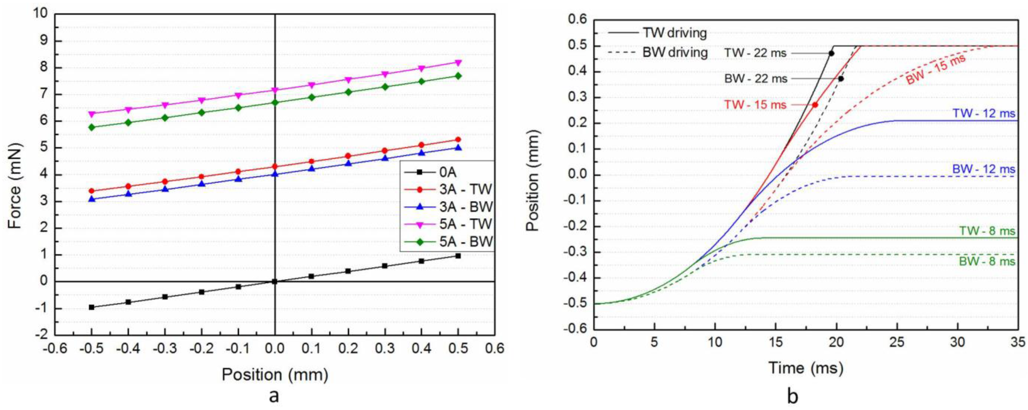
Figure 2a represents the horizontal components (
x and
y) of the total force (
FTotal) exerted on the MPM as function of its position between two discrete positions (located at ±0.5 mm) for different driving current values (0 A, 3 A, and 5 A). The forces obtained using the two wires (TW or BW) are represented. When there is no driving current (0 A), the total force exerted on the MPM is due to the magnetic holding force only. The holding force value of ±1 mN is then visible when the MPM is in discrete positions (±0.5 mm). When the MPM is in the central position (0 mm), the total force exerted on it is null because the magnetic attractions of the FPMs are perfectly equilibrated. When a driving current is used, the initial curve is upward shifted. The shift corresponds to the added electromagnetic driving force. The value of the electromagnetic forces obtained with the TW and BW are given in
Table 1. The electromagnetic force obtained with the BW is 7.1% lower than the one obtained with the TW due to the distance between the two wires (
d3 –
d2).
An important property of a digital actuator is that, under standard conditions, the mobile part should not stop in an intermediate position located between the discrete positions [
9]. For the presented actuator, if the provided energy is not enough (pulse duration too short and/or current magnitude too small), the MPM can stop between the two discrete positions due to the friction between the MPM and the fixed part. This effect is shown in
Figure 2b, where the MPM position as function of time with a 3 A driving current is represented for different pulse durations and using the TW (straight lines) and BW (dashed lines) to switch. If the pulse duration is shorter than 15 ms, the MPM does not reach the +0.5 mm discrete position. For the pulse durations of 8 ms and 12 ms, the MPM displacement is more important using the TW (0.26 mm for 8 ms and 0.71 mm for 12 ms) than using the BW (0.19 mm for 8 ms and 0.51 mm for 12 ms) because the driving force generated using the TW is higher than using the BW. With pulse duration of 22 ms, the switching time is lower than the pulse duration, the MPM velocity increases then throughout the switch. With this configuration, the energy consumption is obviously not minimal. A minimization of the energy consumption can be obtained if the pulse stops before the end of the switch and so that the MPM velocity is high enough to reach the target discrete position (see the switch obtained using the BW for a pulse duration of 15 ms). Considering this configuration, the minimal pulse duration values and the corresponding switching times have been determined and are given in
Table 2.
Figure 2.
Simulation results: (a) force exerted on the MPM as function of its position and for different driving current values, and (b) displacement curves of the MPM for different pulse durations.
Figure 2.
Simulation results: (a) force exerted on the MPM as function of its position and for different driving current values, and (b) displacement curves of the MPM for different pulse durations.
Table 2.
Minimal pulse duration and corresponding switching time.
Table 2.
Minimal pulse duration and corresponding switching time.
| Driving Current | Minimal Pulse Duration | Switching Time |
|---|
| TW | BW | TW | BW |
|---|
| 3 A | 13.2 ms | 15.0 ms | 33.3 ms | 34.6 ms |
| 4 A | 8.5 ms | 9.4 ms | 30.6 ms | 31.8 ms |
| 5 A | 6.3 ms | 6.9 ms | 29.1 ms | 30.0 ms |
| 6 A | 5.0 ms | 5.5 ms | 28.2 ms | 28.9 ms |
| 7 A | 4.2 ms | 4.5 ms | 27.2 ms | 27.9 ms |
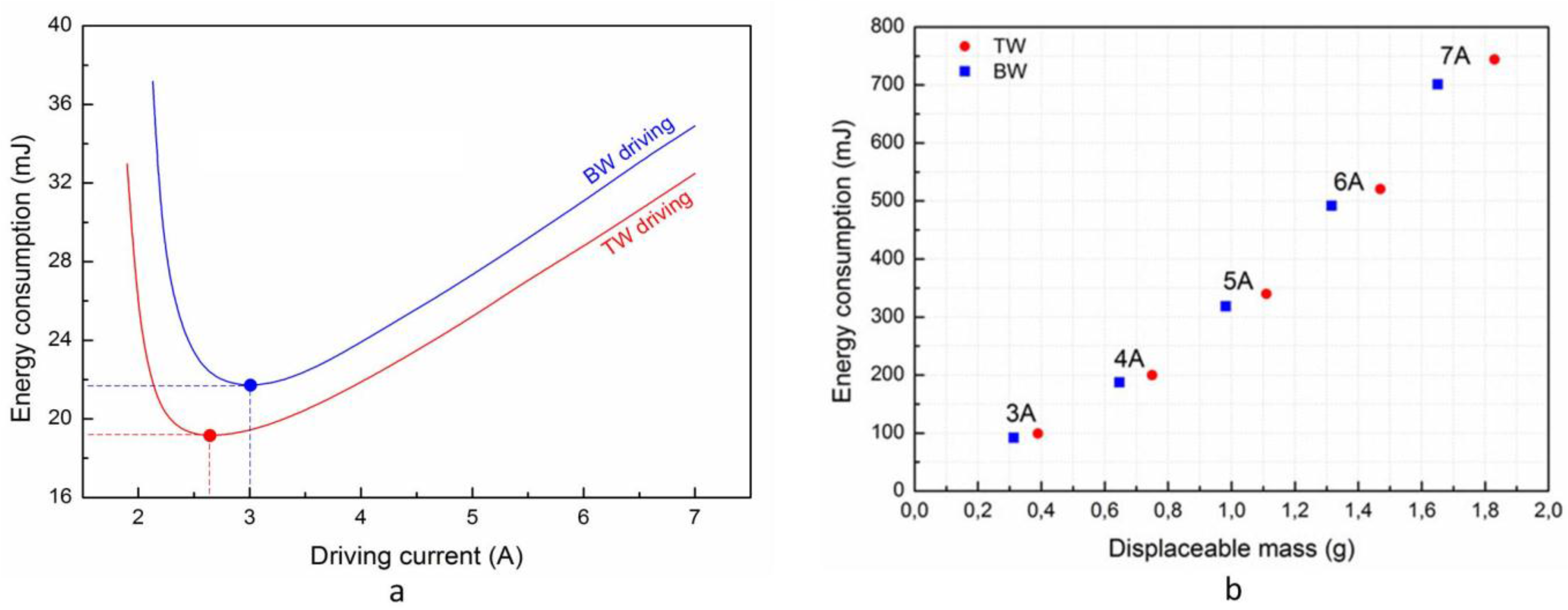
Considering the values given in
Table 2, the energy consumption of the presented digital actuator has been computed for different driving current values and for the two displacement axes (
Figure 3a). The energy consumption (
E) has been determined with Equation (7) where
UDriving is the voltage applied to the considered wire,
IDriving is the driving current through the driving wire and
Δt is the minimal pulse duration (given in
Table 2).
For a given driving current value, the energy consumption is always higher using the BW than the TW because the electromagnetic force generated is lower using the BW than the TW. The two curves present the same evolution and an optimal value is visible at 2.6 A and 3.0 A for the TW and BW, respectively. For driving current lower than these optimal values, the pulse durations increase sharply compared to the reduction of the driving current values. For driving currents higher than these optimal values, the increase of the driving current generates an increase of the energy consumption more important than the decrease due to the reduction of the pulse duration. For the optimal driving current values, the minimal energy consumption of the digital actuator is 19.1 mJ and 21.9 mJ for the x-axis (TW driving) and the y-axis (BW driving) respectively.
Figure 3.
Simulation results: (a) energy consumption as function of the driving current value and (b) energy consumption as function of the displaceable mass for different driving current values.
Figure 3.
Simulation results: (a) energy consumption as function of the driving current value and (b) energy consumption as function of the displaceable mass for different driving current values.
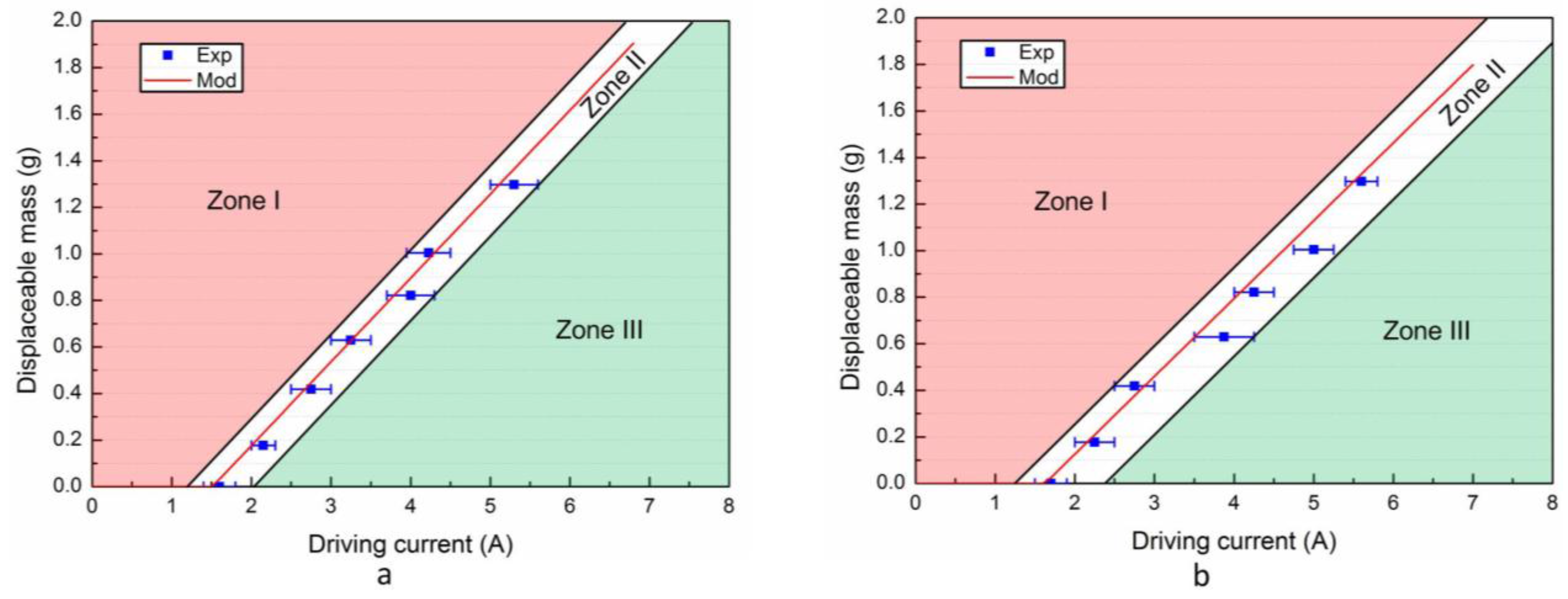
Using the model, the maximum displaceable mass has been determined for different driving current values and for the two displacement axes (
Figure 3b). The maximal displaceable mass by the MPM is obtained with the highest experimentally-available current value (7 A) and is 1.83 g and 1.65 g using the TW and BW, respectively. For each driving current value, the energy consumption has also been computed considering these added masses. For a given current value (e.g., 7 A), the pulse duration is indeed higher for the TW (95.4 ms) than for the BW (89.9 ms) because of the higher added mass (1.83 g for TW and 1.65 g for BW).
5. Application
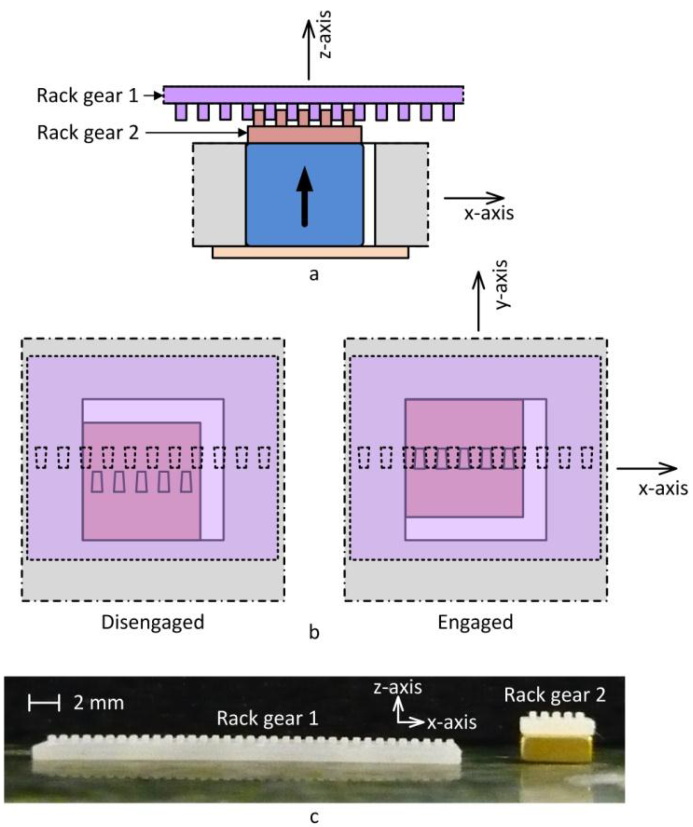
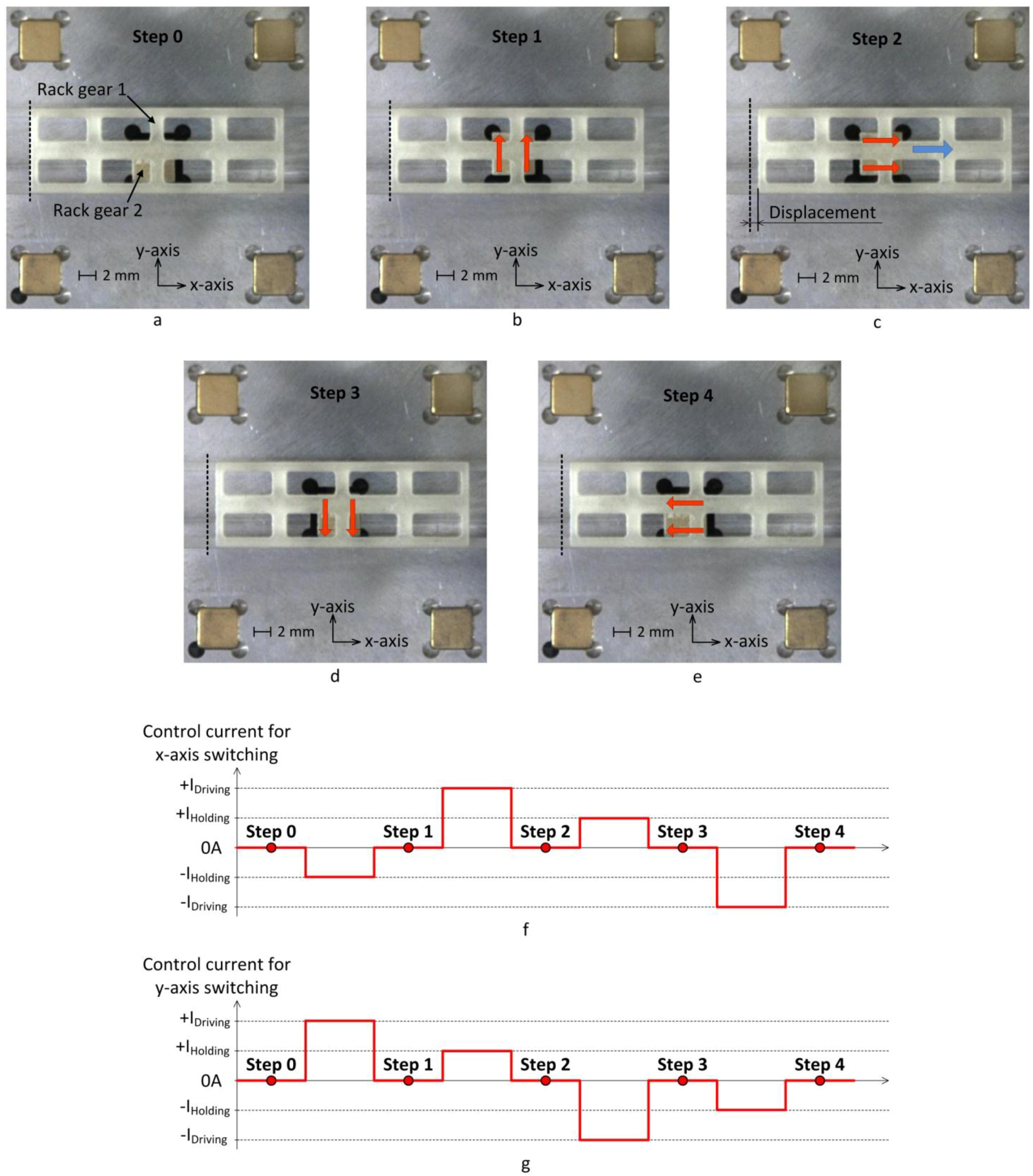
An application of the digital actuator is presented in this section. This application consists of a linear conveyor able to realize long displacement and takes advantage of the high precision and of the two displacement directions of the actuator. In this application, two rack gears are used (
Figure 10a): rack gear 1 is placed on the top side of the actuator, which corresponds to the mobile part of the conveyor, and rack gear 2 is fixed on the top side of the MPM. During the functioning of the conveyor, the two rack gears can be engaged or disengaged as represented in
Figure 10b. The high precision of the digital actuator is an important property for this application because it ensures the engaging/disengaging of the two rack gears without fail at each step. When the two rack gears are engaged, the movement of the MPM generates a displacement of the conveyor mobile part (rack gear 1). For this application, two orthogonal displacement directions are needed: one direction for the actuation and one for the engaging/disengaging of the two rack gears. With the same current value, the electromagnetic force generated with the TW (
x-axis switching) is higher than with the BW (
y-axis switching). The
x-axis has then been chosen for the actuation direction because a high actuation force can be necessary if the mass of the conveyed part is important. On the other hand, the required force during the engaging/disengaging phases is smaller so that the
y-axis (switching using the BW) has been used for this direction.
An experimental test has been realized to validate the principle of this linear conveyor. The two rack gears have been manufactured using rapid prototyping techniques and are shown in
Figure 10c. The geometrical properties of the two rack gears and teeth are given in
Table 5. In order to facilitate the engaging/disengaging phases, the teeth have a trapezoidal shape. Eight apertures have been fabricated in rack gear 1 in order to reduce its mass and to see the displacement of rack gear 2 during the functioning (visible in
Figure 11a).
The
Figure 11 represents a displacement sequence with the experimental prototype. This sequence is composed of four steps. In the initial position, the two rack gears are disengaged and the MPM is located in the (
–xMPM;
–yMPM) discrete position (
Figure 11a). At the first step, the MPM switches in the
+y direction and reaches the (
–xMPM;
+yMPM) discrete position (
Figure 11b) in order to engage the two rack gears. At the second step, the MPM switches in the
+x direction and reaches the (
+xMPM;
+yMPM) discrete position (
Figure 11c). During this step, the rack gear 1 is moved from a distance corresponding to the MPM stroke. At the third step, the two rack gears are disengaged then the MPM switches in the
–y direction and reaches the (
+xMPM;
–yMPM) discrete position (
Figure 11d). At the fourth step, the MPM reaches the initial position (
–xMPM;
–yMPM) by switching in the
–x direction (
Figure 11e) then a new sequence can be realized. A representation of the current signals for
x-axis switching (TW) and
y-axis switching (BW) used for the displacement sequence are presented in
Figure 11f,g, respectively. During the sequence, driving and holding currents are used in order to ensure properly the engaging/disengaging of the two rack gears and the displacement of the rack gear 1. Using this experimental setup, displacements of 30 mm (using the total length of rack gear 1) and a displacement velocity up to 7.5 mm/s have been achieved.
Figure 10.
Principle of a linear conveyor based on the digital actuator: (a) side view, (b) top view, (c) picture of the two rack gears.
Figure 10.
Principle of a linear conveyor based on the digital actuator: (a) side view, (b) top view, (c) picture of the two rack gears.
Table 5.
Rack gears properties.
Table 5.
Rack gears properties.
| Rack gears dimensions |
| Rack gear 1 | Rack gear 2 |
| Length (along x-axis) | 30 mm | 5 mm |
| Width (along y-axis) | 10 mm | 5 mm |
| Thickness (along z-axis) | 1.5 mm | 1.5 mm |
| Number of teeth | 35 | 5 |
| Pitch | 0.85 mm | 0.85 mm |
| Tooth dimensions |
| Length (along x-axis) | 0.33 mm to 0.36 mm (trapeze shape) |
| Width (along y-axis) | 0.5 mm |
| Thickness (along z-axis) | 0.5 mm |
Figure 11.
Displacement sequence of the linear conveyor: (a, b, c, d, and e) pictures of the prototype during the displacement sequence, (f) control signal for x-axis switching used for the sequence, (g) control signal for y-axis switching used for the sequence.
Figure 11.
Displacement sequence of the linear conveyor: (a, b, c, d, and e) pictures of the prototype during the displacement sequence, (f) control signal for x-axis switching used for the sequence, (g) control signal for y-axis switching used for the sequence.


