
Review on the Nonlinear Modeling of Hysteresis in Piezoelectric Ceramic Actuators
1
Changchun Institute of Optics, Fine Mechanics and Physics, Chinese Academy of Sciences, Changchun 130033, China
2
University of Chinese Academy of Sciences, Beijing 100049, China
*
Authors to whom correspondence should be addressed.
Actuators 2023, 12(12), 442; https://doi.org/10.3390/act12120442
Submission received: 8 October 2023
/
Revised: 18 November 2023
/
Accepted: 21 November 2023
/
Published: 28 November 2023
(This article belongs to the Special Issue Shape Memory Alloys and Piezoelectric Materials and Their Applications)
Abstract
:Piezoelectric ceramic actuators have the advantages of fast response speed and high positioning accuracy and are widely used in micro-machinery, aerospace, precision machining machinery, and other precision positioning fields. However, hysteretic nonlinearity has a great influence on the positioning accuracy of piezoelectric ceramic actuators, so it is necessary to establish a hysteretic model to solve this problem. In this paper, the principles of the Preisach model, the Prandtl Ishilinskii (PI) model, the Maxwell model, the Duhem model, the Bouc–Wen model, and the Hammerstein model and their application and development in piezoelectric hysteresis modeling are described in detail. At the same time, the classical model, the asymmetric model and the rate-dependent model of these models are described in detail, and the application of the inverse model corresponding to these models in the feedforward compensation is explained in detail. At the end of the paper, the methods of inverse model acquisition and control frequency of these models are compared. In addition, the future research trend of the hysteresis model is also prospected. The ideas and suggestions highlighted in this paper will guide the development of piezoelectric hysteresis models.
1. Introduction
Piezoelectric materials can be traced back to 1880 [1]. Under external forces, the internal lattice of a crystal undergoes deformation, causing the centers of positive and negative charges to no longer coincide, resulting in a potential difference and causing the crystal to no longer be neutral. This phenomenon, called the piezoelectric effect, was discovered by the Curie brothers (Pierre Curie and Jacques Paul Curie) and is shown in Figure 1.
In contrast, in 1881, Pierre Curie and Jacques Paul Curie soon experimentally confirmed the inverse piezoelectric effect predicted by Gabriel Lippmann [1]: when an electric field is applied to a piezoelectric material, the piezoelectric material produces a geometrical deformation, as shown in Figure 2.
The geometric deformation generated by piezoelectric materials is approximately proportional to the strength of the electric field. By using the inverse piezoelectric effect, the piezoelectric material can be used as a displacement driver.
Today, a variety of piezoelectric materials have been found, such as piezoelectric single crystals such as quartz, titanium germanate and lithium gallium oxide; organic piezoelectric polymers such as PVDF (vinylidene fluoride); and piezoelectric ceramics such as PbZrxTi1-xO3 (lead zirconate titanate for short PZT), BaTiO3 (barium titanate), and PbTiO3 (lead titanate). Among them, piezoelectric ceramics are the most-used piezoelectric materials in the field of precision positioning [2,3,4,5,6,7]. Piezoelectric ceramic actuators have the advantages of high displacement resolution, fast response speed, small size, and low noise. They have been widely used in fields such as micro-angular rate gyros [8], nondestructive testing (NDT) [9], micro/nanopositioning systems [10,11,12,13,14,15], atomic force microscopes [16,17], aerospace [18,19], medical devices [20], micro-pumps/valves [21,22,23,24,25], and imaging systems [26,27]. However, their hysteresis characteristics greatly affect their positioning accuracy. Therefore, it is necessary to model the hysteresis characteristics of piezoelectric ceramic actuators and use the model to improve the positioning accuracy of the actuator.
This paper mainly introduces some common hysteresis models of piezoelectric ceramic actuators and their development, including the Preisach model [28,29,30,31,32,33,34,35,36,37,38,39,40,41,42,43,44], the Prandtl Ishilinskii (PI) model [45,46,47,48,49,50,51,52,53,54,55,56,57,58,59,60,61,62,63,64], the Maxwell model [65,66,67,68,69,70,71,72,73,74,75,76,77], the Duhem model [78,79,80,81,82,83,84,85,86,87,88,89,90], the Bouc–Wen model [91,92,93,94,95,96,97,98,99,100,101,102,103,104,105], and the Hammerstein model [106,107,108,109,110,111]. Section 2 and Section 3 briefly introduce the microstructure of piezoelectric ceramics [2,112,113] and the hysteresis characteristics of piezoelectric ceramic actuators [114,115,116,117,118,119], Section 4 briefly introduces the inverse model and feedforward compensation [57,59], Section 5, Section 6, Section 7, Section 8, Section 9 and Section 10 provide a detailed introduction to each model, Section 11 compares each model, and Section 12 is a summary.
2. Microstructure and Poling of Piezoelectric Ceramics
From a microscopic perspective, piezoelectric ceramics can be subdivided into many grains with different lattice orientations, each of which is composed of many periodically arranged crystal cells. The crystal cell is composed of positively charged ions and negatively charged ions. Under the action of temperature changes, electric fields, or mechanical loads (stress), the relative positions of positive and negative charge centers in piezoelectric ceramic crystal cells can be changed [2,112].
Take the common BaTiO3 piezoelectric ceramic material as an example. When the material temperature T decreases from a value higher than the Curie temperature Tc (about 120 °C–130 °C) to a value lower than the Curie temperature, the internal crystal cells of the material will change from cubic cells with overlapping positive and negative charge centers to tetragonal cells with non-overlapping positive and negative charge centers, as shown in Figure 3. When the material is below the Curie temperature, the non-coincidence of the positive and negative charge centers in the crystal cell can lead to spontaneous polarization and strain. The small domains composed of adjacent crystal cells with the same spontaneous polarization direction are called Weiss domains or ferroelectric domains [112]. Due to the random polarization direction of a single ferroelectric domain, piezoelectric ceramics at this time cannot produce piezoelectric or inverse piezoelectric effects at a macroscopic level.
When BaTiO3 piezoelectric ceramics are subjected to a high-voltage electric field (about 2 kV/mm) higher than the coercive electric field intensity, the polarization direction of each ferroelectric domain will roughly align with the direction of the electric field. Then, even if the external electric field is removed, the polarization direction of the ferroelectric domain will not completely return to its initial state, but will remain a portion at the macro level. This portion of polarization that is retained is called irreversible or remanent polarization, and this process is called poling, as shown in Figure 4. The polarized piezoelectric ceramics have piezoelectric properties due to the presence of remanent polarization. The coercive electric field strength refers to the critical electric field strength that can initiate domain switching [2,113].
Similar to the coercive electric field strength, piezoelectric ceramics also have the coercive stress. That is to say, a sufficiently large mechanical load (stress) can generate residual strain, and the critical stress that can initiate domain switching is called coercive stress. Although a sufficiently large mechanical load (stress) can change the relative positions of the positive and negative charge centers of a single cell, the final polarization state of each domain is random, so mechanical loads cannot polarize piezoelectric ceramics at the macro level [113]. Piezoelectric ceramics are generally polarized through an externally strengthened DC electric field.
3. Hysteresis Characteristics of Piezoelectric Ceramic Actuators
The concept of hysteresis was first proposed by Scottish scientist Alfred Ewing in 1882 while studying ferromagnetic materials [114]. Later, more and more scholars found that the hysteresis phenomenon exists not only in ferromagnetic materials but also in many fields such as magnetic materials and ferroelectric materials [116], and piezoelectric ceramics belong to a kind of ferroelectric materials.
The hysteresis characteristics of piezoelectric ceramic actuators used for high-precision positioning are shown in Figure 5. The voltage boost curve and the voltage drop curve in the figure are not straight and do not coincide, and there is a multi-value mapping between voltage and displacement. This multi-value mapping relationship shows that the current displacement of the piezoelectric ceramic actuator is related not only to the current voltage value but also to the historical voltage value. Meanwhile, the step-up curve and step-down curve are asymmetrical about the symmetry axis of the diagram, which brings some difficulty to the establishment of hysteresis model.
On the other hand, temperature, mechanical load, and frequency of input voltage all have an impact on the piezoelectric hysteresis curve. Among them, temperature and mechanical load can affect the sensitivity of piezoelectric actuators; that is, under other unchanged conditions, the average slope of the hysteresis curve varies at different temperatures [117,118] or different mechanical loads [119], and different mechanical loads may also affect the width of the hysteresis curve, as shown in Figure 6 and Figure 7a. The frequency of the input voltage will have an impact on the width of the hysteresis curve. The higher the frequency, the wider the hysteresis curve, as shown in Figure 7b.
It is worth mentioning that the hysteresis phenomenon of piezoelectric actuators is closely related to their microstructure. As previously mentioned, temperature changes and mechanical loads can alter the relative positions of positive and negative charge centers in the crystal cells of piezoelectric ceramics, which seems to be a microscopic explanation for the influence of temperature and load on the slope of the hysteresis curve. The influence of the frequency of the input voltage on the width of the hysteresis curve is mainly related to the vibration of the piezoelectric actuator [112,122]. References [112,121,123] point out that the switching and movement of domain walls are the main reasons for hysteresis nonlinearity. The finite element method (FEM) divides an object into finite elements for numerical simulation, with each element corresponding to a grain. This method can effectively simulate the switching and movement of domain walls [121,124] and can accurately model nonlinear phenomena, including rate-independent and rate-dependent hysteresis [125,126]. The finite element method is very suitable for simulation research and can be used to simulate the physical properties of piezoelectric materials well. However, the discrete workload of this method is very large [125], and it is not widely used in the field of hysteresis nonlinear modeling of piezoelectric ceramic actuators.
In addition to hysteresis characteristics, piezoelectric ceramic actuators also exhibit creep characteristics. Creep characteristics refer to the phenomenon of slow drift that occurs when the input voltage stabilizes at a certain value after increasing or decreasing voltage, but the output displacement of a piezoelectric ceramic actuator cannot immediately stabilize in a short time. As time increases, the displacement gradually tends to stabilize. Compared with creep characteristics, hysteresis characteristics have a greater impact on the nonlinearity of the actuator. This article mainly discusses the nonlinear hysteresis modeling method of piezoelectric ceramic actuators.
4. Inverse Model
The forward model of the piezoelectric ceramic actuator generally takes voltage as input and displacement as output, and the inverse model takes expected displacement as input and voltage as output. As shown in Figure 8, represents the expected displacement, is the output voltage of the inverse model and the input voltage of the actuator, and represents the output displacement of the actuator. In a control system, the inverse model can be used for feedforward compensation [127,128,129,130] or combined with PID and other algorithms for compound control [131,132,133].
There are generally two methods for obtaining inverse models: one is to directly take the actuator output displacement data as the model input and the actuator input voltage as the model output during parameter identification so that the identified model can be directly used as the inverse model, such as the PI model based on the Stop operator [57]. The other is to first identify the parameters of the positive model, and then indirectly calculate the inverse model parameters using mathematical equations, such as the PI model based on the Play operator [52].
5. Preisach Model
5.1. Model Introduction
The classical Preisach model is a kind of weighted superposition to describe the hysteresis model based on the operator. This model was proposed by F. Preisach [34] in 1935 to describe the hysteresis of ferromagnetic materials. Later, the author of reference [35] extended the application of the model, pointing out that the Preisach model can describe not only the magnetization of ferromagnets but also the polarization of ferroelectrics. The model is formed by the weighted superposition of multiple relay operators. The mathematical expression of relay operators [28,29,30,31,32,33,37] is as follows:
where is the input of the operator (which is also the input of the model), is the output of the operator, and and represent the threshold of the operator’s rise and fall.
Figure 9a can be used to characterize Equations (1) and (2) above. When the operator input is greater than the rise threshold , the operator output rises to +1. If the operator input is less than the drop threshold , the operator output drops to −1. If is between the two thresholds, the output of the operator neither rises nor falls and only keeps the current state unchanged until changes to the rising threshold or the falling threshold , and the output of the operator changes accordingly.
Then, several relay operators are multiplied by corresponding weights for superposition, and the Preisach model can be obtained, as shown in Figure 9b.
The model expression is as follows:
where is the output of the model and is the weight.
It can be seen from the above model expression that the integral region of the double integral is the part on the plane. Meanwhile, in practical engineering applications, the input signal is bounded. Assuming that is the upper bound of the input signal and is the lower bound of the input signal, the integration region of the model is determined, as shown in the following Figure 10a.
According to the value of relay operator , the integral region can be divided into positive and negative parts, as shown in Figure 10b, the region of “+1” for is , and the region of “−1” for is . The integration region in the graph is composed of countless coordinate points, where each coordinate point represents a relay operator, its vertical coordinate represents the ascending threshold of the operator, and its horizontal coordinate represents the descending threshold of the operator, and each operator corresponds to a weight .
The output displacement corresponding to Figure 10b can be expressed as
When the voltage changes continuously from , as shown in Figure 11, the positive and negative conditions of the integral region on the Preisach plane change according to Figure 12. If all the weights are equal to 1, then the difference between the yellow and white areas in Figure 12 represents the current output displacement of the Preisach model. By observing the change in the integral region in Figure 12, the following findings can be observed. When the voltage increases, the -axis leading to the rise threshold should be mainly concerned, and the area of the yellow part gradually increases along the -axis from bottom to top. When the voltage drops, attention should mainly be paid to the -axis, which dominates the drop threshold, and the area of the yellow part gradually decreases from right to left.
5.2. Model Development
Because of the double integral in the expression, it is difficult to identify the continuous Preisach model. Therefore, it is necessary to discretize the Preisach model. The author of reference [36] proposed a numerical implementation method of the discrete Preisach model, which avoided the process of second-order derivative weight evaluation and the subsequent double integral output displacement calculation in the process of model identification, thus reducing the difficulty of modeling.
The author of reference [38] changed the output of the relay operator in Equation (1) from “+1” and “−1” to “+1” and “0” according to the polarization characteristics of the piezoelectric ceramic actuator, which made the integral region change from the original first, second, and third quadrants to the first quadrant, as shown in Figure 13b. Since the operator output of the “T−“ part of the integral region is “0”, which makes Equation (4) become , the model is further simplified.
The numerical implementation method of the Preisach model is also given in the literature [38].
As shown in Figure 14a, represents the displacement change caused by the voltage increasing from bottom to top ; as in Figure 14b, represents the displacement change caused by the voltage decreasing from the right to the left . Therefore, each change corresponds to the corresponding triangle area in the figure. The final integral region consists of three parts, , and , so the total displacement at this time can be expressed by Equation (5) or (6):
The meanings of the parameters in Equations (5) and (6) are the same as before. Consider the more general case, ; then, the total displacement of the actuator is the sum of the double integral of the region , which can be expressed by Equation (7).
Consider the opposite of Figure 14e, where the voltage is perpendicular to the β axis instead of the α axis, and the total displacement has another expression:
Equations (7) and (8) are the numerical implementation methods of the discrete Preisach model, in which the value of in the Preisach function is measured experimentally.
The author of reference [40] provided a value table of a piezoelectric actuator through experiments, as shown in Figure 15. If the voltage is not in the table, the corresponding Preisach function value can be obtained through linear interpolation.
The author of reference [42] proposed a diagonally weighted Preisach model for the problem that linear interpolation cannot obtain accurate values, in which the basic elements constituting the Preisach triangle are considered to have weights along their diagonal lines. The continuity of the discrete Preisach model is improved.
On the other hand, due to the poor rate-dependent description ability of the Preisach model, the author of reference [39] introduced the derivative of voltage with respect to time into the weight of the double integral and then combined it with the neural network to establish a dynamic model of a piezoelectric actuator. The maximum error between the output of the model and the actual displacement was less than 5% after testing the input signal at a maximum of 32 Hz. The author of reference [43] proposed a modified Preisach model to improve the rate-dependent description ability by using a HOFODE (hysteresis operator of a first-order differential equation) instead of the relay operator in the Preisach model. They also implemented a rate-dependent model of piezoelectric ceramic actuators using the MDRNN (modified diagonal recurrent neural networks) with a similar structure to the modified Preisach model. Unlike references [39,43], which use neural networks to replace the Preisach model, the author of reference [44] added a frequency weight to the classical Preisach model formula and used Fast Fourier Transform (FFT) to approximate the values of the frequency weight and density function, establishing a rate-dependent hysteresis model for piezoelectric actuators.
In terms of the inverse model, inspired by the study [57], the author of reference [60] proposed a Preisach inverse model, as shown in Figure 16b. The hysteresis curve of the piezoelectric ceramic actuator is counterclockwise. To compensate for this clockwise hysteresis, the hysteresis curve of the inverse model should be clockwise, as shown in Figure 16a. However, the hysteresis loop of the relay operator is counterclockwise and is not suitable for direct use as an inverse model. The author of reference [60] defined a clockwise relay operator that is complementary to the original relay operator, as shown in Equations (9) and (10), which can be used to construct inverse Preisach models.
where represents the clockwise relay operator that can be used to construct the Preisach inverse model, and the meanings of other parameters are consistent with those in Equations (1) and (2).
6. PI (Prandtl Ishilinskii) Model
The PI model is improved using the Preisach model. The output displacement of the piezoelectric ceramic actuator is obtained through the linear superposition of each operator output. The classical PI model has two basic operators: the Play operator and the Stop operator [51,53,55].
6.1. Classical PI Model Based on the Play Operator
6.1.1. Basic Principles of the Play Operator
The Play operator is also known as the Backlash operator [51]. Figure 17 describes its principle, where the displacement of car A is the input u of the operator, the displacement of car B is the output v of the operator, and the threshold r of the operator is the gap between cars A and B. If the absolute value of the operator input u is less than or equal to the threshold r, then the operator output v is 0; if the input u is greater than r, then the output v is u − r; if the input u is less than −r, then the output v is u + r; the Play operator of the PI model simulates the hysteresis characteristics of piezoelectric ceramics in this way.
The continuous input signal is divided into M cells in the time domain , where . On each cell , is monotonically continuous and M is a positive integer (); then, the i-th Play operator [45,47,48,49,50] expression can be expressed by Equation (11).
where ; is the number of operators; is the output of the i-th operator; is the input for the operator at time t; is the output of the previous sampling period of the i-th operator; T is the sampling period; , which is the initial value of the i-th operator; is the threshold calculation equation; and indicates the maximum input.
Finally, the output displacement of the model is obtained by summing the outputs of each operator multiplied by the corresponding weights. The discrete mathematical expression of the PI model based on the Play operator can be expressed by Equation (12):
where is the model output displacement; are the weights corresponding to each operator, and the weights of each operator are obtained from the experimental data through parameter identification.
The model diagram corresponding to Equation (12) is shown in Figure 18:
6.1.2. Illustrate Play Operator Superposition Process
The superposition process of the Play operator is shown in Figure 19. The displacement of car is still used as the model input; the displacements of cars represent the output of each operator; and the gaps between cars represent the operator thresholds. Finally, as shown in Equation (12), the final output displacement can be obtained by multiplying each operator output with its corresponding weight . Among them, the displacement of car is equivalent to the input voltage of piezoelectric ceramics, and the output displacement obtained through superposition is equivalent to the output displacement of piezoelectric ceramics.
As shown in Figure 20, the green output displacement curve in the figure is formed from the superposition of each weighting operator’s outputs .
Combined with Figure 19, it can be found that the rising stage of the model output displacement can be seen in Figure 20. As input gradually increases and exceeds the threshold of each operator, each operator is activated in turn, and the output value of the operator starts to change in turn. When the input signal reaches , the absolute value of the output of each operator also reaches a peak.
In the decreasing stage of the model output displacement, except for the operator with a threshold value of “0”, the output of other operators will remain unchanged in a certain period of time, which is due to the existence of reverse gap, as shown in Figure 19. At this time, the reverse gap of each operator is , so the output value of the corresponding operator will start to change only when . In other words, the absolute value of the output of each operator in Figure 20 will only start to decrease to zero after being constant for a short time. Of course, the output of some other operators will remain unchanged if they fail to meet the conditions due to the large threshold value. The above is the more detailed working process of the Play operator.
6.2. A Classical PI Model Based on Stop Operator
The classical PI model based on the Stop operator can be explained using the spring slider shown in Figure 21. Similarly, the displacement of point A is taken as the operator input, and the spring force of slider B is taken as the operator output . When the spring force does not exceed the breakaway force , the operator output , where is the spring stiffness. When the spring force exceeds the breakaway force , the operator outputs . The shift of this segment at point can be regarded as the threshold value in the Play operator; thus, the difference between the Stop operator and the Play operator can be found. The Play operator means that when the input reaches the threshold, the output begins to increase. The Stop operator means that after the input is increased to the threshold, the output will no longer increase, so the Stop operator is called the Stop operator; that is, the output will stop increasing after reaching the threshold. Similar to the Play operator, the PI model based on the Stop operator [45,46] can be expressed as follows:
where is input the operator at time t; is the threshold of the i-th operator; is the output of the i-th operator; is the output of the previous sampling period of the i-th operator; T is the sampling period; , which is the initial value of the i-th operator; and is the weight of the i-th operator.
6.3. The Complementary Relationship between the Play Operator and the Stop Operator
The Play operator and the Stop operator are complementary, the sum of the output of the two operators is equal to the input signal , and the Play operator is represented by :
where ; represents operator output; represents the output of the operator in the previous period. The meanings of other symbols are the same as in Equation (11).
The Stop operator is represented by :
where ; represents the operator output; and represents the output of the operator in the previous period. The meanings of other symbols are the same as in Equation (13).
Therefore, the complementary relationship between the two operators [116] can be expressed as
This complementary relationship is manifested in different hysteresis directions on the input and output graphs of operators. As shown in Figure 22, the clockwise cycle characteristic of the Stop operator in the graph is an important reason why the PI model based on the Stop operator can be directly used as the inverse model.
6.4. Different Expressions of Classical PI Models
In practical applications, both the Play operator and the Stop operator generally use the discrete form shown in Equation (18) [61]:
where is the model output displacement; is the output of the i-th operator; is the number of operators; values are the weights corresponding to the i-th operator; and the weights of each operator are obtained from the experimental data through parameter identification. The corresponding continuous form of Equation (18) is [61]
where is the model output; is a weight function; is the operator output; and is the threshold value; The upper limit R is usually infinity.
In many studies [53,56,58,116,135], the discrete PI model is also expressed as
where is the model output; is the input for the model; is the initial load curve constant greater than zero; is the same as , which represents the weight of the i-th operator; is the same as , which represents the output of the i-th operator; the threshold in this case , [58]; and the Play operator output in Equation (20) can also be replaced by the Stop operator output .
Equations (18) and (20) are not fundamentally different, and both describe hysteresis through basic operator superposition. The additional term is equivalent to the product of an operator with a zero threshold and its weight, as shown in Figure 19; is equivalent to an operator with a zero threshold, and is equivalent to the weight of the operator. The corresponding continuous form of the above equation can be expressed as [53,56,58,116,135]
where is the model output; is the input for the model; is a constant greater than zero; is the same as , which represents the weight function; is the same as , which represents the output of operator. Similarly, the Play operator can also be replaced by the Stop operator .
6.5. The Development of the PI Model
For both the classical PI model based on the Play operator and the PI model based on the Stop operator, the hysteresis curves fitted by them are symmetric and cannot describe the asymmetric hysteresis characteristics of piezoelectric ceramic actuators. Therefore, many scholars have proposed asymmetric PI models.
The author of reference [55] proposed an asymmetric generalized Play operator using and , two different envelope functions to represent the falling and rising segments of the Play operator, respectively, as shown in Figure 23.
The input and output of the operator are represented in the figure. The generalized Play operator can be expressed as
The superposition summation equation based on the generalized Play operator is the same as the classical PI model shown in Equation (21), which will not be repeated here. The envelope functions and of the generalized Play operator can be selected according to the actual hysteresis curve of the actuator, such as the exponential function, the polynomial function, and the trigonometric function.
The author of reference [56] et al. divided the classical Play operator into two parts: the right Play operator and the left Play operator.
Right Play operator equation:
Left Play operator equation:
In the equation,
where and , respectively, represent the maximum value and minimum value of each lifting period input by the operator, and and , respectively, represent the maximum value and minimum value of each lifting period output by the operator. The expression of the asymmetric PI model is
where is the weight of the initial load curve; is the number of operators; and and are the weights of the right Play operator and the left Play operator, respectively. The basic idea of the asymmetric PI model [56] is similar to that of the generalized Play operator in the literature [55], both of which separately represent the rising and falling segments of the hysteresis curve, but the mathematical expressions of the two are more complex than the literature in [61].
The author of reference [61] proposed a PI model of the Asymmetric Unilateral Backlash operator based on the classical Backlash operator (i.e., the Play operator). The expression of the operator is relatively simple:
where is the operator output, is the operator input, is the threshold value, is the asymmetric correction coefficient, is the operator output of the previous period, is the model output of each operator after multiplication by the corresponding weight, and is the corresponding weight of each operator output. From the perspective of the expression, the main difference between Equation (27) and the classical PI model based on Play operator is that the first term of the function min changes from “” to “”, which makes the ascending and descending segments of the operator no longer symmetric and thus can describe the asymmetric hysteresis characteristics.
In addition, the classical PI model is a static model, which cannot describe the hysteresis of the actuator under high-frequency input. Therefore, the author of reference [53] proposed a frequency-dependent PI model to describe the dynamic hysteresis curve of the actuator. The main idea of this model is to take the operator threshold in the classical PI model as a function of the input frequency so that the model can describe the response of the actuator under different input frequencies. The expression of the operator threshold is as follows:
In the equation, , , , , and they are constants. The order of the threshold is determined by , and is the derivative of the input signal.
Accordingly, the rate-dependent Play operator is expressed as
The rate-dependent PI model is expressed as follows:
where is the input signal discrete according to the sampling period , and the input signal is continuous in ( ); represent the model output; is the weight of the dynamic threshold ; and is the output of the rate-dependent Play operator;
where , are positive constants identified by experimental data, and their values are related to the material type of the actuator.
The author of reference [62] pointed out that hysteresis is independent of rate, but as the driving frequency approaches the resonant frequency, structural vibration increases. Reference [62] considers the combination effect of hysteresis and vibration from a phenomenological perspective. The dead zone operator is weighted and stacked together with the Play operator to obtain a modified PI operator, and a function related to the slope of the hysteresis curve is introduced into the weight of the modified PI operator. The final experiment shows that this method can perform rate-dependent modeling on the hysteresis phenomenon of a 40 Hz driving frequency.
Unlike the authors of references [53,62], the authors of reference [63] did not use operator thresholds related to input frequency or introduce slope-related functions in operator weights. Instead, they first proposed an MPI model composed of a one-side Play (OSP) operator, and then introduced two envelope functions related to input voltage derivatives in the one-side Play (OSP) operator to obtain an MRPI model. Finally, precise open-loop control under high-frequency input was achieved using the MRPI inverse model.
The author of reference [64] used the Gaussian Process (GP) to model piezoelectric actuators and compared the proposed GP hysteresis model with the MPI model in reference [63]. The results showed that the proposed GP hysteresis model had better rate-dependent description ability.
In terms of the inverse model, the author of reference [57] proved that the PI model based on the Stop operator can be used as inverse model. The hysteresis direction of the Stop operator (clockwise) is opposite to the direction of the actual piezoelectric hysteresis curve (counterclockwise), which is a key reason why the PI model based on the Stop operator can be used as an inverse model.
The direction of the Play operator is the same as that of the actual piezoelectric curve, so the PI model based on the Play operator is not suitable for direct use as an inverse model [60] and can be indirectly solved using mathematical equations. In addition, the inverse model and the original model are both PI models, but the threshold and weight of the inverse model are different from the original model. The equation based on the PI inverse model of the Play operator is given in the literature [52], as shown in Equations (34) and (35):
where is the output voltage of the inverse model; represents the weights of each operator in the inverse model; is the expected displacement of the input; is the weight of each operator of the inverse model; is the sampling period; and is the output voltage of the inverse model in the previous period.
7. Maxwell Model
7.1. Generalized Maxwell-Slip Model
The Maxwell model was proposed by physicist and mathematician James C. Maxwell et al. in 1868 to describe viscoelastic phenomena [65,66]. The Maxwell model itself is a physical model that describes the relationship between displacement and force [65,66], and each parameter has a relatively clear physical meaning. Similar to the classical PI model based on the Stop operator, the Maxwell model [73,74,75,76,77] can be interpreted as a system composed of multiple massless Elasto-Slide elements in parallel. A single Elasto-Slide element is shown in Figure 24.
The output equation for a single Elasto-Slide element is
Each parameter in the equation corresponds to Figure 24, represents the output force of the i-th Elasto-Slide element; represents the stiffness of the i-th spring; represents input displacement; represents the displacement of the i-th slider; indicates the friction force to be overcome by the movement of the i-th slider.
In simple terms, when the absolute value of the spring force is less than the friction force , which is needed to be overcome by the slider movement, the output force is equal to the spring force; the output force is equal to the maximum friction force in all cases except when the rate of change in the input is 0. The relationship between input displacement and output force of the basic element of the model is shown in Figure 25 below.
Finally, the n massless Elasto-Slide elements are summed in parallel to obtain the total output force, which is also the model output force, as follows:
When the number of elements (operators) n approaches infinity, the above model consisting of n Elasto-Slide elements is called the generalized Maxwell-Slip model. The n parallel elements corresponding to Equation (37) are shown in Figure 26.
It is worth mentioning that the generalized Maxwell-Slip model is not only limited to describing the hysteresis relationship between displacement and force but also can describe many rate-independent hysteresis phenomena, such as the hysteresis between charge and voltage, entropy and temperature, and magnetic flux and magnetomotive force [65].
7.2. Development of the Generalized Maxwell-Slip Model
The hysteresis described by generalized Maxwell is centrosymmetric, but the actual hysteresis curve of piezoelectric ceramic actuators is asymmetric. Therefore, the author of reference [67] considered the actual stiffness of the actuator and the equivalent stiffness generated by the actuator capacitance on the basis of the original model, and connected and in series and then in parallel with the original model to improve the model’s accuracy. Then, a nonlinear spring unit is connected in parallel to describe the asymmetric hysteresis curve of the actuator. In reference [67], the inverse model equation for compensation control is further given.
The accuracy of the generalized Maxwell model increases with the increase in the number of Elasto-Slide elements. However, increasing the number of elements to improve the accuracy will also increase the number of parameters that need to be identified, making it difficult for the model to balance the accuracy and complexity. The author of reference [70] pointed out that the PI model based on the Play operator could be represented by the Elasto-Slide elements in series or the Elasto-Slide elements with negative stiffness in parallel, while the PI model based on the Stop operator could be represented by the Elasto-Slide elements with positive stiffness in parallel, indicating that the generalized Maxwell-Slip model and the classical PI model are mathematically equivalent. However, the Maxwell model has better interpretability. At the same time, it [70] replaces the Elasto-Slide elements in the generalized Maxwell model with elastic and sliding elements and proposes a distributed parameter Maxwell-Slip model (DPMS), which takes into account the accuracy and complexity of the model as much as possible.
7.3. Maxwell Resistor Capacitor Model (MRC Model)
Maxwell models can be represented by multiple Elasto-Slide elements in parallel. It can also be expressed by the nonlinear MRC resistive capacitor proposed by the author of reference [65,66]. The Maxwell-Slip model represents the lag between displacement and force, and the MRC resistance capacitance model (hereinafter referred to as the MRC model) represents the lag between charge and voltage. The MRC model, which consists of a nonlinear resistor and a nonlinear capacitor in series, can be used in conjunction with electromechanical models of piezoelectric ceramic actuators. The mathematical expression of the MRC model is as follows:
where is the amount of charge accumulated by the nonlinear capacitance , and is the output voltage of MRC model. The remaining parameters are the electrical simulations of each parameter in Equations (36) and (37) [65].
The explanation given by the literature [65] for the parameters in Equations (38) and (39) may not be easy to understand, but a more understandable explanation is given below. The MRC model in the literature [65], which consists of a nonlinear resistor and a nonlinear capacitor in series, is disassembled into MRC elements composed of several linear resistors and capacitors, and then these elements are simply superimposed to better explain the physical meaning of the parameters in Equations (38) and (39). It should be noted that the “superimposed” here does not refer to the MRC elements in series or in parallel but still regards each element as an independent individual, but it needs to assume that the input charge of each element is the same, and then the output voltage of each element is superimposed and summed. In combination with Figure 27, the parameters in Equations (38) and (39) can be explained as follows: is the voltage of the i-th capacitor; is the input charge of the capacitor in the MRC element; and is the amount of overflow charge consumed by the resistor after the capacitor is fully charged. is the capacity of the i-th capacitor; represents the voltage value when the i-th capacitor is fully charged; is the current in the series circuit; and is the output of the total voltage to the model.
The electromechanical model of the piezoelectric ceramic actuator combined with the MRC module is shown below.
In Figure 28, the electrical part on the left to the mechanical part on the right can be associated with the inverse piezoelectric effect of the piezoelectric ceramic actuator; that is, the output displacement can be controlled through the input voltage of the piezoelectric ceramic. The mechanical part on the right to the electrical part on the left can be linked to the positive piezoelectric effect; that is, the displacement caused by the external force can change the voltage. That is to say, the displacement is not only related to the input voltage of the electrical part but also to the external force suffered by the mechanical part, and there is electromechanical coupling between the two parts. The mathematical expression of the electromechanical model of the actuator is composed of four parts, mechanical, electrical, and electromechanical conversion and nonlinear hysteresis, as follows:
- (1)
- Linear second-order dynamic equation of the mechanical part:where are the mass, damping, and stiffness of the actuator, respectively; represents actuator displacement; is the output force of the actuator; and represents the load from the outside. The dynamic equation here describes the vibration of the system, and the rate-dependent description ability of the entire model mainly comes from this.
- (2)
- The total voltage u and total charge q of the input electrical part arewhere is the voltage at both ends of MRC module in Figure 28 and Figure 27; is the voltage at both ends of the transducer in the electrical part of the model; is the capacitor in parallel with the transducer; and is the charge of the transducer.
- (3)
- Electromechanical conversion relationship:where and represent the electromechanical conversion ratios of actuator voltage to force and displacement to charge, respectively. and can also be uniformly represented by T [65,66,67], but in reality, they have different physical interpretations, and it is best to use different symbols to represent them [68,72].
- (4)
- The nonlinear hysteresis part:is the nonlinear hysteresis part of the actuator, represented by the MRC model described in Equations (38) and (39). In addition to using the MRC model, the nonlinear hysteresis part can also use models such as the Preisach model and the PI model.
The biggest advantage of the above electromechanical model of the actuator using the MRC module is that the physical meaning of each parameter is relatively clear, each parameter is relatively interpretable, and the dynamic equation contains first-order terms and second-order terms, so the rate-dependent control is realized in the literature [65] to a certain extent. However, the disadvantages of this model are that there are more model parameters and more complex model expressions. Meanwhile, MRC model is not fundamentally different from the generalized Maxwell model. Like the classical PI model, it can only describe symmetrical hysteresis.
7.4. Development of MRC Model
The author of reference [68] combined the molecular dipole with the Weiss domain theory and used an ideal capacitor and a voltage-limiting capacitor to further explain the hysteresis characteristics of piezoelectric ceramics and the MRC model. Then, by removing the first- and second-order terms of the dynamic equation, a modified MRC model is obtained, which only describes the low-frequency behavior of the piezoelectric ceramics. Finally, considering the hysteresis and creep characteristics of the actuator, fractional-order dynamics is integrated into the modified MRC model, and a fractional-order MRC model (FOMRC) is proposed to describe the hysteresis and creep phenomena at the same time, and its inverse model is established for compensation control.
8. Duhem Model
The Duhem model was proposed by physicist P. Duhem in 1897 as a differential equation model to describe hysteresis phenomena [78,82,85]. Coleman and Hodgdon [79] proposed a simplified Duhem model based on the hysteresis characteristics of ferromagnetic materials, called the Coleman–Hodgdon (C-H) model [81,82,88,89,90] or the classical Duhem model [86]. The model expression is as follows:
where is the output displacement, is the input voltage, is a normal number, and and are the function selected according to different types of hysteresis curves.
The most difficult part of the model is to find the function of and , which are suitable for describing the hysteresis characteristics of the actuator [83]. The author of reference [83] selected polynomial functions to approximate and according to the famous Weierstrass first approximation theorem and used recursive least squares to identify parameters and coefficients of polynomials.
In addition, because the classical Duhem model is a differential-equation-based model, it is not easy to construct its inverse model [81,82]. Taking the sliding-mode control as an example, the author of reference [81] proposed a method to reduce unknown hysteresis without constructing an inverse model. The author of reference [84] identified the parameters of the Duhem model using a method similar to [83] and directly applied the identification results to the Duhem inverse model, eliminating the complicated inverse process.
In order to further improve the accuracy of the model, the author of reference [85] proposed an improved Duhem model, whose equation is as follows:
where is the output displacement of the actuator, is the linear displacement component, is the hysteresis displacement component, is the input voltage, and , , , and are the shape parameters of the hysteresis curve.
On the other hand, the Duhem model shown in Equation (46) cannot accurately describe the hysteresis characteristics under high-frequency input signals, so the author of reference [87] introduced a fractional-order operator on the basis of Equation (46). A fractional-order Duhem model is proposed to improve the rate-dependent description ability.
9. Bouc–Wen Model
9.1. Model Introduction
The Bouc–Wen model was proposed by Robert Bouc in 1967 to describe hysteretic nonlinear systems, and Yi-kwei Wen extended it in 1976 [93,98,135], thus establishing the classical Bouc–Wen model. The Bouc–Wen model can be regarded as a variant of the Duhem model [80]. The model equation is as follows [100,101,102,103,104,105]:
where represents model output displacement; is the model input voltage; is the linear term coefficient; represents nonlinear term; and can be regarded as a differential equation transformed from the “” transformation in the Duhem model [80]. , , and determine the width and shape of the hysteresis curve, and these four parameters are introduced in detail using hysteresis curves in literature [91,96,98].
9.2. Model Development
The classical Bouc–Wen model’s ability to describe the asymmetric rate dependence of hysteresis loops is also not perfect. Therefore, many scholars have also proposed asymmetric and rate-dependent Bouc–Wen models.
The author of reference [91] combined the differential equation of piezoelectric dynamics with the Bouc–Wen model to establish a hysteresis dynamic model of a three-layer piezoelectric bimorph beam. The author of reference [96] applied the improved Bouc–Wen model proposed in reference [91] to the rate-dependent modeling of piezoelectric actuators. Moreover, by comparing the error between the model output and experimental data, it was found that the model has good accuracy in the frequency range of 10–120 kHz.
The author of reference [94] introduced an asymmetric term into the nonlinear differential equation of the classical Bouc–Wen model to enhance the ability of the model to capture asymmetric hysteresis. The model equation is as follows:
where is the asymmetric factor; the meanings of other parameters are consistent with Equation (48).
Based on the literature [94], the author of reference [95] introduced the frequency factor into the dynamic differential equation to make the generalized Bouc–Wen model proposed by them have both asymmetric and rate-dependent description capabilities. The model equation is as follows:
where is the model output displacement; is the initial displacement of actuator; and represent velocity and acceleration, respectively; , , and are, respectively, the mass, damping and stiffness of the actuator; is the piezoelectric coefficient; is the frequency factor; t is time; is the input voltage; is nonlinear hysteretic force; is similar to impulse; the meanings of the corresponding , , , and parameters are consistent with those in Equation (48); is the derivative of the input voltage with respect to time; and is the asymmetric factor.
The author of reference [97] combined the classical Bouc–Wen model with a fractional-order creep model in the form of a transfer function, and simultaneously described the hysteretic and creep behavior of piezoelectric actuators below 1 Hz.
In terms of inverse models, the author of reference [93] proposed an inverse multiplication structure, which can be used to obtain the inverse model of Bouc–Wen. By writing the nonlinear term “” in Equation (47) as , Equation (47) can be transformed into , represents the expected displacement, and represents the input voltage of the actuator, which is the inverse multiplication structure in literature [93]. However, the sum in the inverse multiplication structure is difficult to determine with and at the same time, which leads to the problem of algebraic loops. Although the introduction of time delay and the low-pass filter can solve the algebraic cycle problem, it will also bring certain errors [60].
In order to solve the algebraic cycle problem of the inverse model, the author of reference [99] modified the last two terms of in the classical Bouc–Wen model and proposed a modified Bouc–Wen(MBW) model:
where is the output of the MBW hysteresis operator modified from ; , , are positive constants that determine the shape of the hysteresis curve; and represents the input voltage of the piezoelectric actuator. Then, on the basis of Equation (52), a series of weighted polynomial (WP) functions are used to describe the asymmetric hysteresis:
where and , respectively, represent the weight and order of the weighted polynomial function . Finally, in order to capture rate-dependent hysteresis, a dynamic linear model is connected after the WPMBW model formed by Equations (52) and (53), as shown in Figure 29.
The equation for the dynamic linear model is as follows:
where represents the output and and represent the coefficient of the derivative of and the coefficient of the derivative of , respectively.
The Inverse WPMBW model corresponding to Equations (52)–(54) are shown in Equation (55) and Figure 30 (the order of the weighted polynomial function in reference [99] is taken as L = 2):
For more details on the WPMBW model, see reference [99].
10. Hammerstein Model
The Hammerstein model was proposed by mathematician A. Hammerstein in 1930 to describe dynamic nonlinear systems [106]. The Hammerstein model is more like a framework, as shown in Figure 31. It is composed of the static nonlinear part and the dynamic linear part in series, which are used to describe the rate-independent and rate-dependent characteristics of the piezoelectric actuator, respectively. In the figure, and represent the input voltage and output displacement, respectively. The static nonlinear part can use the classical PI model [109], the modified PI model [106], and the Bouc–Wen model [108], as well as other forms such as least square support vector machine, neural network, and polynomial [106]. The dynamic linear part can use the ARX (auto-regressive model with exogenous input) model as shown in Equations (56) and (57) [108].
where represents the unit delay operator. Combined with Figure 31, where is the error term caused by the random disturbance , the discrete transfer function between exogenous input and output of the ARX model can be expressed as
In fact, as shown in Figure 29, the WPMBW model and dynamic linear model in reference [99] have already used the framework of the Hammerstein model in series. In addition, the Hammerstein model has been used by many researchers because of its excellent rate-dependent hysteresis ability to describe piezoelectric actuators. The author of reference [106] used the Hammerstein model in series with the Modified PI model and the ARX model to describe the rate-dependent hysteresis characteristics of the actuator. The author of reference [107] proposed an additive cascaded model based on the Hammerstein model. In the static nonlinear part, the PI model based on the Play operator was used to describe the hysteresis of the actuator, and the transfer function of the dynamic linear part was divided into two parts: low frequency and high frequency, used to describe creep and vibration, respectively. The author of reference [108] used the Hammerstein model composed of the Bouc–Wen model and the ARX model to establish the rate-dependent hysteresis model for piezoelectric ceramic actuators. In order to describe the rate-dependent hysteretic and creep behavior of actuators, the author of reference [109] combined the Hammerstein model with a fractional-order model for describing creep, in which the Hammerstein model was formed by connecting the classical PI model with the ARX model. The author of reference [110] superimposed a butterfly hysteresis operator based on exponential function with the asymmetric Bouc–Wen model to form a hybrid static hysteresis model, which was used as the static nonlinear part of Hammerstein model to improve the modeling accuracy of the static part, while the dynamic linear part still used the second-order transfer function. Compared with integer-order systems, fractional-order systems can capture the dynamic characteristics of actuators more effectively [111]. Therefore, the author of reference [111] proposed a fractional-order Hammerstein model to better describe the rate-dependent characteristics of the actuator, in which the fractional-order transfer function was used for the dynamic linear part and the Bouc–Wen model was used for the static linear part.
11. Model Comparison
The double integral in the Preisach model needs to be discretized in practical applications, and the accuracy of the discretized model largely depends on the number of operators. However, increasing the number of operators will inevitably lead to an increase in the computational complexity of the model. At the same time, this method of improving model accuracy by increasing the number of operators has an upper limit. When the number of operators increases to a certain number, the model accuracy will no longer be improved. The Preisach model cannot accurately describe the hysteresis phenomenon of piezoelectric ceramic actuators under high-frequency input signals, but its static performance is good and can describe the rate-independent hysteresis phenomenon.
Due to the complexity of the Preisach model, the classical PI model simplifies the Preisach model, making it easier to establish, but it is unable to describe the asymmetric rate-dependent hysteresis curve of the actuator. As a result, many asymmetric PI models [55,56,59,61] and rate-dependent PI models [53,59] have emerged one after another. On the other hand, the classical PI model still describes hysteresis phenomena through operator superposition, so the model accuracy is also closely related to the number of operators.
There is essentially no difference between the Elasto-Slide Element of the Maxwell model and the two basic operators of the PI model [70]. So, similar to the PI model, the Maxwell model is not as capable of describing high-frequency input signals as the Duhem model, the Bouc–Wen model, and other models mentioned later. However, the parameters of the Maxwell model have a clearer physical meaning and better interpretability than the PI model.
The Duhem model does not use operator superposition to describe hysteresis characteristics but instead uses differential equations, which makes the model accuracy not limited by the number of operators. As long as suitable functions can be found, different types of hysteresis can be described, but finding such functions is not easy, and polynomial functions can usually be used [83].
Compared with the aforementioned operator class models such as the Preisach model, the PI model, the Maxwell model, etc., as one of the branches of the Duhem model, the Bouc–Wen model only needs to select reasonable parameter values in the model to describe the hysteresis characteristics of piezoelectric ceramic actuators in various situations, without increasing the number of operators. The number of model parameters are relatively small, so the Bouc–Wen model appears simpler.
Finally, as a block-oriented model, the Hammerstein model can simultaneously model the asymmetric hysteresis, rate-dependent hysteresis, and creep of piezoelectric actuators by combining various basic models in series, but it is also more complex than other basic models.
Based on the literature we have reviewed, the approximate frequency range that can maintain good performance and the inverse model acquisition methods of the several basic models in this article has been showed in Table 1. As the Hammerstein model is composed of basic models in series, it will not be included in the table.
12. Summary
This article first briefly introduces the piezoelectric effect and inverse piezoelectric effect of piezoelectric materials and points out the importance of establishing an actuator hysteresis model. Then, a brief introduction was given to the microstructure of piezoelectric ceramics and the hysteresis characteristics of actuators. The effects of temperature, load, and input voltage frequency on the slope and width of the hysteresis curve were discussed, and two methods for obtaining the inverse model were introduced.
Subsequently, a detailed introduction was given to some common hysteresis models: firstly, operator class models were introduced, which are not inherently complex but gradually become more complex as the number of operators increases. Among the three models of the Preisach, the PI and the Maxwell, the Preisach model should be more complex than the other two models, but it has good static description ability. The PI model is simpler than the Preisach model, and its complementary the Play operator and the Stop operator provide inspiration for the inverse models of many other models. The Maxwell model is similar to the PI model, but the parameters of the Maxwell model have clear physical meanings. Then, two differential class models were introduced, whose model accuracy does not depend on the number of operators, so, to some extent, differential class models are simpler than operator class models. The subsequent Hammerstein model concatenates various basic hysteresis models with dynamic transfer functions, giving the model better dynamic description ability.
Finally, the above basic hysteresis models were compared, and it was found that the Bouc–Wen model may have better rate-dependent description ability than other basic models in the text. In addition, the fractional-order Hammerstein model can simultaneously describe hysteresis and creep, which may become a focus of future research. The main contribution of this article is to summarize the nonlinear modeling methods for the hysteresis of piezoelectric ceramics, which can help researchers and engineers choose appropriate models for their own applications.
Author Contributions
Conceptualization Y.D. and D.L.; Search and analysis of the related literature, Y.D. and D.L.; Writing—original draft preparation, Y.D. and D.L.; Project administration, D.W. All authors have read and agreed to the published version of the manuscript.
Funding
This work is supported by the Natural Science Foundation of Jilin Province (Grant No. 20230101066JC), National Natural Science Foundation of China (Grant No. 12103052) and civil aerospace pre-research project of China (Grant No. D050101).
Data Availability Statement
No new data were created or analyzed in this study. Data sharing is not applicable to this article.
Conflicts of Interest
The authors declare no conflict of interest. The funders had no role in the design of the study; in the collection, analyses, or interpretation of data; in the writing of the manuscript; or in the decision to publish the results.
References
- Arnau, A.; Soares, D. Fundamentals of Piezoelectricity. In Piezoelectric Transducers and Applications; Vives, A.A., Ed.; Springer: Berlin/Heidelberg, Germany, 2008; pp. 1–38. [Google Scholar]
- Kaltenbacher, M. Piezoelectric Systems. In Numerical Simulation of Mechatronic Sensors and Actuators; Springer: Berlin/Heidelberg, Germany, 2007; pp. 243–266. [Google Scholar]
- Jaffe, B.; Cook, W.R.; Jaffe, H. Chapter 12—Applications of Piezoelectric Ceramics. In Piezoelectric Ceramics; Jaffe, B., Cook, W.R., Jaffe, H., Eds.; Academic Press: Cambridge, MA, USA, 1971; pp. 271–280. [Google Scholar]
- Lai, Z.L.; Liu, X.D.; Geng, J.; Li, L. Sliding mode control of hysteresis of piezoceramic actuator based on inverse Preisach compensation. Opt. Precis. Eng. 2011, 19, 1281–1290. [Google Scholar] [CrossRef]
- Uchino, K. Antiferroelectric Shape Memory Ceramics. Actuators 2016, 5, 11. [Google Scholar] [CrossRef]
- Liu, Y.; Zhang, S.; Yan, P.; Li, H. Finite Element Modeling and Test of Piezo Disk with Local Ring Electrodes for Micro Displacement. Micromachines 2022, 13, 951. [Google Scholar] [CrossRef] [PubMed]
- Chen, Y. Hysteresis Modeling and Nonlinear Control of Piezoelectric Actuators. Ph.D. Thesis, Nanjing University of Aeronautics and Astronautics, Nanjing, China, 2013. [Google Scholar]
- Wu-fa, L.; Zhen-bang, G.; Zhen, J. Design of micro piezoelectric ceramic rod angular rate gyro. Opt. Precis. Eng. 2006, 14, 439–442. [Google Scholar]
- Xu, C.; Xie, J.; Zhang, W.; Kong, Q.; Chen, G.; Song, G. Experimental Investigation on the Detection of Multiple Surface Cracks Using Vibrothermography with a Low-Power Piezoceramic Actuator. Sensors 2017, 17, 2705. [Google Scholar] [CrossRef] [PubMed]
- Cao, X.-T.; Li, D.-Q.; Li, H.-W.; Lin, G.-Y.; Yang, W.-F. Precision drive and position control of non-resonance piezoelectric stack linear motor. Opt. Precis. Eng. 2017, 25, 2139–2148. [Google Scholar] [CrossRef]
- Xu, S.A.; Xie, M.; Sun, J.; Chen, L.; Wang, G.R. Long range nano-positioning system based on optoelectronic phase-shift for piezoelectric actuator. Opt. Precis. Eng. 2014, 22, 2773–2778. [Google Scholar] [CrossRef]
- Hu, Y.; Zhang, H.; Ni, K. Mini-piezo-element drive microactuator based on triangular amplification. Opt. Precis. Eng. 2022, 30, 2094–2099. [Google Scholar] [CrossRef]
- Li, J.; Deng, J.; Liu, Y.; Yu, H.; Tian, X.; Li, K. A Linear Piezoelectric Actuator Based on Working Principle of Three-Petal Mouth of a Rabbit. IEEE Trans. Ind. Electron. 2022, 69, 5091–5099. [Google Scholar] [CrossRef]
- Gao, X.; Deng, J.; Zhang, S.; Jing, L.; Liu, Y. A Compact 2-DOF Micro/Nano Manipulator Using Single Miniature Piezoelectric Tube Actuator. IEEE Trans. Ind. Electron. 2022, 69, 3928–3937. [Google Scholar] [CrossRef]
- Deng, J.; Liu, Y.; Zhang, S.; Li, J. Development of a Nanopositioning Platform With Large Travel Range Based on Bionic Quadruped Piezoelectric Actuator. IEEE/ASME Trans. Mechatron. 2021, 26, 2059–2070. [Google Scholar] [CrossRef]
- Fairbairn, M.W.; Moheimani, S.O.R.; Fleming, A.J. Q Control of an Atomic Force Microscope Microcantilever: A Sensorless Approach. J. Microelectromechanical Syst. 2011, 20, 1372–1381. [Google Scholar] [CrossRef]
- Eslami, B.; Solares, S.D. Experimental approach for selecting the excitation frequency for maximum compositional contrast in viscous environments for piezo-driven bimodal atomic force microscopy. J. Appl. Phys. 2016, 119, 084901. [Google Scholar] [CrossRef]
- Li, M.; Yuan, J.; Guan, D.; Chen, W. Application of piezoelectric fiber composite actuator to aircraft wing for aerodynamic performance improvement. Sci. China Technol. Sci. 2011, 54, 395–402. [Google Scholar] [CrossRef]
- Yu, Z.; Wang, Y.; Cao, K.; Chen, H. Hysteresis compensation and composite control for Piezoelectric actuator. Opt. Precis. Eng. 2017, 25, 2113–2120. [Google Scholar] [CrossRef]
- Yang, J.; Zhang, Q.; Xu, T. A Novel Piezoelectric Ceramic Actuator with Scissoring Composite Vibration for Medical Applications. Appl. Sci. 2019, 9, 4637. [Google Scholar] [CrossRef]
- Mohith, S.; Karanth, P.N.; Kulkarni, S.M. Experimental investigation on performance of disposable micropump with retrofit piezo stack actuator for biomedical application. Microsyst. Technol. 2019, 25, 4741–4752. [Google Scholar] [CrossRef]
- Hirooka, D.; Yamaguchi, T.; Furushiro, N.; Suzumori, K.; Kanda, T. Highly responsive and stable flow control valve using a PZT transducer. In Proceedings of the 2016 IEEE International Ultrasonics Symposium (IUS), Tours, France, 18–21 September 2016; pp. 1–3. [Google Scholar]
- Li, H.; Liu, J.; Li, K.; Deng, J.; Liu, Y. Development of a High-Pressure Self-Priming Valve-Based Piezoelectric Pump Using Bending Transducers. IEEE Trans. Ind. Electron. 2022, 69, 2759–2768. [Google Scholar] [CrossRef]
- Li, H.; Liu, J.; Feng, Y.; Deng, J.; Liu, Y. A Broadband, High-Power Resonant Piezoelectric Active-Valve Pump Driven By Sandwich Bending Transducers. IEEE Trans. Ind. Electron. 2023, 70, 9336–9345. [Google Scholar] [CrossRef]
- Li, H.; Liu, Y.; Li, K.; Deng, J.; Feng, Y.; Liu, J. A resonant piezoelectric proportional valve for high-flowrate regulation operated by a bending sandwich actuator. Sens. Actuators A Phys. 2021, 331, 112971. [Google Scholar] [CrossRef]
- Yuan, G.; Wang, D.H.; Li, S.D. Single piezoelectric ceramic stack actuator based fast steering mirror with fixed rotation axis and large excursion angle. Sens. Actuators A Phys. 2015, 235, 292–299. [Google Scholar] [CrossRef]
- Dai, M.; Ding, H.; Huang, C.; Zhu, Y.; Wang, M. Design of a Panoramic Scanning Device Based on a Piezoelectric Ceramic Stack Actuator and Friction Transmission. Actuators 2022, 11, 159. [Google Scholar] [CrossRef]
- Chen, Y.; Huang, Q.; Wang, H.; Qiu, J. Hysteresis modeling and tracking control for piezoelectric stack actuators using neural-Preisach model. Int. J. Appl. Electromagn. Mech. 2019, 61, 445–459. [Google Scholar] [CrossRef]
- Yu, Y.; Xiao, Z.; Naganathan, N.G.; Dukkipati, R.V. Dynamic Preisach modelling of hysteresis for the piezoceramic actuator system. Inst. Mech. Eng. Part C J. Mech. Eng. Sci. 2001, 215, 511–521. [Google Scholar] [CrossRef]
- Yu, Y.H.; Xiao, Z.H.; Naganathan, N.; Dukkipati, R.V. Preisach modeling of hysteresis for piezoceramic actuator system. Proc. Int. J. Ser. C-Mech. Syst. Mach. Elem. Manuf. 2001, 44, 553–560. [Google Scholar] [CrossRef]
- Zhou, X.; Zhao, J.; Song, G.; De Abreu-Garcia, J. Preisach modeling of hysteresis and tracking control of a Thunder actuator system. In Proceedings of the Smart Structures and Materials 2003: Modeling, Signal Processing, and Control, San Diego, CA, USA, 25 September 2003; pp. 112–125. [Google Scholar]
- Li, L.I.; Liu, X.; Wei, W.; Huo, C. Generalized nonlinear Preisach model for hysteresis nonlinearity of piezoceramic actuator and its numerical implementation. Opt. Precis. Eng. 2007, 15, 706–712. [Google Scholar]
- Gao, X.; Ren, X.; Gong, X.a.; Huang, J.; IEEE. The Identification of Preisach Hysteresis Model Based on Piecewise identification method. In Proceedings of the 2013 32nd Chinese Control Conference (CCC), Xi’an, China, 26–28 July 2013; pp. 1680–1685. [Google Scholar]
- Preisach, F. Über die magnetische Nachwirkung. Z. Für Phys. 1935, 94, 277–302. [Google Scholar] [CrossRef]
- Everett, D.H.; Whitton, W.I. A general approach to hysteresis. Trans. Faraday Soc. 1952, 48, 749–757. [Google Scholar] [CrossRef]
- Mayergoyz, I. Mathematical models of hysteresis. IEEE Trans. Magn. 1986, 22, 603–608. [Google Scholar] [CrossRef]
- Mayergoyz, I.D. The Classical Preisach Model of Hysteresis. In Mathematical Models of Hysteresis; Mayergoyz, I.D., Ed.; Springer New York: New York, NY, USA, 1991; pp. 1–63. [Google Scholar]
- Ge, P.; Jouaneh, M. Modeling hysteresis in piezoceramic actuators. Precis. Eng. 1995, 17, 211–221. [Google Scholar] [CrossRef]
- Song, D.; Li, C.J. Modeling of piezo actuator’s nonlinear and frequency dependent dynamics. Mechatronics 1999, 9, 391–410. [Google Scholar] [CrossRef]
- Lv, Y.; Wei, Y. Study on open-loop precision positioning control of a micropositioning platform using a piezoelectric actuator. In Proceedings of the Fifth World Congress on Intelligent Control and Automation (IEEE Cat. No.04EX788), Hangzhou, China, 15–19 June 2004; Volume 1252. pp. 1255–1259. [Google Scholar]
- Zhou, X.; Yang, S.; Qi, G.; Hu, X. Tracking control of piezoceramic actuators by using preisach model. In Proceedings of the ICMIT 2005: Control Systems and Robotics, Chongqing, China, 29 September 2006; p. 604248. [Google Scholar]
- Nguyen, P.-B.; Choi, S.-B.; Song, B.-K. A new approach to hysteresis modelling for a piezoelectric actuator using Preisach model and recursive method with an application to open-loop position tracking control. Sens. Actuators A Phys. 2018, 270, 136–152. [Google Scholar] [CrossRef]
- Dang, X.; Tan, Y. Neural networks dynamic hysteresis model for piezoceramic actuator based on hysteresis operator of first-order differential equation. Phys. B Condens. Matter 2005, 365, 173–184. [Google Scholar] [CrossRef]
- Xiao, S.; Li, Y. Modeling and High Dynamic Compensating the Rate-Dependent Hysteresis of Piezoelectric Actuators via a Novel Modified Inverse Preisach Model. IEEE Trans. Control. Syst. Technol. 2013, 21, 1549–1557. [Google Scholar] [CrossRef]
- Fang, C.; Guo, J.; Xu, X.; Jiang, Z.; Wang, T. Compensating controller for hysteresis nonlinerity of piezoelectric ceramics. Opt. Precis. Eng. 2016, 24, 2217–2223. [Google Scholar] [CrossRef]
- Hassani, V.; Tjahjowidodo, T. A hysteresis model for a stacked-type piezoelectric actuator. Mech. Adv. Mater. Struct. 2017, 24, 73–87. [Google Scholar] [CrossRef]
- Fan, Y.; Tan, U.-X. A Feedforward Controller With Neural-Network Based Rate-Dependent Model For Piezoelectric-Driven Mechanism. In Proceedings of the 2016 Ieee International Conference on Robotics and Biomimetics (ROBIO), Qingdao, China, 3–7 December 2016; pp. 1558–1563. [Google Scholar]
- Al Janaideh, M.; Tan, X.; IEEE. Adaptive Estimation of Threshold Parameters for a Prandtl-Ishlinskii Hysteresis Operator. In Proceedings of the 2019 American Control Conference (ACC), Philadelphia, PA, USA, 10–12 July 2019; pp. 3770–3775. [Google Scholar]
- Zuo, S.; Wang, H.; Zhou, D.; Gao, J. Solution of Parameters for PI Inverse Model Based on Geometric Method. Electron. Opt. Control. 2019, 26, 47–50, 60. [Google Scholar]
- Janaideh, M.A.; Xu, R.; Tan, X. Adaptive Estimation of Play Radii for a Prandtl-Ishlinskii Hysteresis Operator. IEEE Trans. Control. Syst. Technol. 2021, 29, 2687–2695. [Google Scholar] [CrossRef]
- Krasnosel’skiǐ, M.A.; Pokrovskiǐ, A.V. Front Matter. In Systems with Hysteresis; Krasnosel’skiǐ, M.A., Pokrovskiǐ, A.V., Eds.; Springer: Berlin/Heidelberg, Germany, 1989; pp. I–XVIII. [Google Scholar]
- Kuhnen, K. Modeling, Identification and Compensation of Complex Hysteretic Nonlinearities: A Modified Prandtl-Ishlinskii Approach. Eur. J. Control. 2003, 9, 407–418. [Google Scholar] [CrossRef]
- Janaideh, M.A.; Rakheja, S.; Su, C.Y. Characterization of Rate Dependent Hysteresis of Piezoceramic Actuators. In Proceedings of the 2007 International Conference on Mechatronics and Automation, Harbin, China, 5–8 August 2007; pp. 550–555. [Google Scholar]
- Chen, X.; Hisayama, T. Adaptive Sliding-Mode Position Control for Piezo-Actuated Stage. IEEE Trans. Ind. Electron. 2008, 55, 3927–3934. [Google Scholar] [CrossRef]
- Janaideh, M.A.; Su, C.Y.; Rakehja, S. Modeling hysteresis of smart actuators. In Proceedings of the 2008 5th International Symposium on Mechatronics and Its Applications, Amman, Jordan, 27–29 May 2008; pp. 1–4. [Google Scholar]
- Jiang, H.; Ji, H.L.; Qiu, J.H.; Chen, Y.S. A Modified Prandtl-Ishlinskii Model for Modeling Asymmetric Hysteresis of Piezoelectric Actuators. IEEE Trans. Ultrason. Ferroelectr. Freq. Control. 2010, 57, 1200–1210. [Google Scholar] [CrossRef] [PubMed]
- Li, Z.; Farhan, O.; Rakheja, S.; Su, C.-Y.; Janaideh, M. Compensation of play operator-based Prandtl-Ishlinskii hysteresis model using a stop operator with application to piezoelectric actuators. Int. J. Adv. Mechatron. Syst. 2012, 4, 25–31. [Google Scholar] [CrossRef]
- Nie, Z.; Fu, C.; Liu, R.; Guo, D.; Ma, Y. Asymmetric Prandtl–Ishlinskii Hysteresis Model for Giant Magnetostrictive Actuator. J. Adv. Comput. Intell. Intell. Inform. 2016, 20, 223–230. [Google Scholar] [CrossRef]
- Yu, Z.; Wu, Y.; Fang, Z.; Sun, H. Modeling and compensation of hysteresis in piezoelectric actuators. Heliyon 2020, 6, e03999. [Google Scholar] [CrossRef] [PubMed]
- Li, Z.; Shan, J.; Gabbert, U. A Direct Inverse Model for Hysteresis Compensation. IEEE Trans. Ind. Electron. 2021, 68, 4173–4181. [Google Scholar] [CrossRef]
- Ang, W.T.; Garmon, F.A.; Pradeep, K. Khosla Modeling on Rate-Dependent Hysteresis Nonlinear Characteristics ofPiezoelectric Stack Actuators. Piezoelectrics Acoustooptics 2022, 44, 907–912. [Google Scholar] [CrossRef]
- Ang, W.T.; Khosla, P.K.; Riviere, C.N. Feedforward Controller With Inverse Rate-Dependent Model for Piezoelectric Actuators in Trajectory-Tracking Applications. IEEE/ASME Trans. Mechatron. 2007, 12, 134–142. [Google Scholar] [CrossRef]
- Yang, M.-J.; Li, C.-X.; Gu, G.-Y.; Zhu, L.-M. Modeling and compensating the dynamic hysteresis of piezoelectric actuators via a modified rate-dependent Prandtl–Ishlinskii model. Smart Mater. Struct. 2015, 24, 125006. [Google Scholar] [CrossRef]
- Tao, Y.-D.; Li, H.-X.; Zhu, L.-M. Rate-dependent hysteresis modeling and compensation of piezoelectric actuators using Gaussian process. Sens. Actuators A Phys. 2019, 295, 357–365. [Google Scholar] [CrossRef]
- Goldfarb, M.; Celanovic, N. Modeling piezoelectric stack actuators for control of micromanipulation. IEEE Control. Syst. Mag. 1997, 17, 69–79. [Google Scholar] [CrossRef]
- Goldfarb, M.; Celanovic, N. A lumped parameter electromechanical model for describing the nonlinear behavior of piezoelectric actuators. J. Dyn. Syst. Meas. Control. Trans. Asme 1997, 119, 478–485. [Google Scholar] [CrossRef]
- Yeh, T.-J.; Lu, S.-W.; Wu, T.-Y. Modeling and Identification of Hysteresis in Piezoelectric Actuators. J. Dyn. Syst. Meas. Control 2005, 128, 189–196. [Google Scholar] [CrossRef]
- Liu, Y.; Shan, J.; Gabbert, U.; Qi, N. Hysteresis and creep modeling and compensation for a piezoelectric actuator using a fractional-order Maxwell resistive capacitor approach. Smart Mater. Struct. 2013, 22, 115020. [Google Scholar] [CrossRef]
- Liu, Y.; Shan, J.; Gabbert, U. Feedback/feedforward control of hysteresis-compensated piezoelectric actuators for high-speed scanning applications. Smart Mater. Struct. 2015, 24, 015012. [Google Scholar] [CrossRef]
- Liu, Y.; Du, D.; Qi, N.; Zhao, J. A Distributed Parameter Maxwell-Slip Model for the Hysteresis in Piezoelectric Actuators. IEEE Trans. Ind. Electron. 2019, 66, 7150–7158. [Google Scholar] [CrossRef]
- Joel, S.; Edward, K. Modeling of Piezoceramic Actuators for Control. In Piezoelectric Actuators; Hu, H., Jianping, L., Eds.; IntechOpen: Rijeka, Balkans, 2021; p. Ch. 5. [Google Scholar]
- Georgiou, H.M.S.; Mrad, R.B. Electromechanical Modeling of Piezoceramic Actuators for Dynamic Loading Applications. J. Dyn. Syst. Meas. Control. 2005, 128, 558–567. [Google Scholar] [CrossRef]
- Dong, W.J.; Sun, B.Y. Observer-based piezoelectric self-sensing actuator. In Proceedings of the International Conference on Sensor Technology (ISTC 2001), Proceedings, Wuhan, China, 10–12 October 2001; pp. 472–475. [Google Scholar]
- Choi, G.S.; Lim, Y.A.; Choi, G.H. Tracking position control of piezoelectric actuators for periodic reference inputs. MECHATRONICS 2002, 12, 669–684. [Google Scholar] [CrossRef]
- Dong, W.; Sun, B.; Cui, Y.; Yang, Z. Study on observer based piezoelectric self-sensing actuator. Chin. J. Mech. Eng. 2002, 38, 80–83. [Google Scholar] [CrossRef]
- Miri, N.; Mohammadzaheri, M.; Chen, L. A comparative study of different physics-based approaches to modelling of piezoelectric actuators. In Proceedings of the 2013 IEEE/ASME International Conference on Advanced Intelligent Mechatronics, Wollongong, NSW, Australia, 9–12 July 2013; pp. 1211–1216. [Google Scholar]
- Xie, S.; Ni, C.; Duan, H.; Liu, Y.; Qi, N.; IEEE. Hybrid Model Based on the Maxwell-Slip Model and a Support Vector Machine for Hysteresis in Piezoelectric Actuators. In Proceedings of the 2020 IEEE/ASME International Conference on Advanced Intelligent Mechatronics (AIM), Boston, MA, USA, 6–9 July 2020; pp. 36–41. [Google Scholar]
- Duhem, P. Die dauernden Aenderungen und die Thermodynamik. I. Z. Für Phys. Chem. 1897, 22U, 545–589. [Google Scholar] [CrossRef]
- Coleman, B.D.; Hodgdon, M.L. A Constitutive Relation For Rate-Independent Hysteresis In Ferromagnetically Soft Materials. Int. J. Eng. Sci. 1986, 24, 897–919. [Google Scholar] [CrossRef]
- Oh, J.; Bernstein, D.S. Semilinear Duhem model for rate-independent and rate-dependent hysteresis. IEEE Trans. Autom. Control. 2005, 50, 631–645. [Google Scholar] [CrossRef]
- Du, J.; Feng, Y.; Su, C.Y.; Hu, Y.M. On the robust control of systems preceded by Coleman-Hodgdon hysteresis. In Proceedings of the 2009 IEEE International Conference on Control and Automation, Christchurch, New Zealand, 9–11 December 2009; pp. 685–689. [Google Scholar]
- Ying, F.; Rabbath, C.A.; Chai, T.; Su, C.Y. Robust adaptive control of systems with hysteretic nonlinearities: A Duhem hysteresis modelling approach. In Proceedings of the AFRICON 2009, Nairobi, Kenya, 23–25 September 2009; pp. 1–6. [Google Scholar]
- Chen, H.; Tan, Y.; Zhou, X.; Dong, R.; Zhang, Y. Identification of Dynamic Hysteresis Based on Duhem Model. In Proceedings of the 2011 Fourth International Conference on Intelligent Computation Technology and Automation, Shenzhen, China, 28–29 March 2011; pp. 810–814. [Google Scholar]
- Chen, H.; Tan, Y.; Zhou, X.; Zhang, Y.; Dong, R. Identification and control of dynamic modeling for piezoceramic actuator. Opt. Precis. Eng. 2012, 20, 88–95. [Google Scholar] [CrossRef]
- He, Y. Research on Improved Duhem Hysteresis Modeling and Control of Piezoelectric Actuator. Master’s Thesis, Taiyuan University of Science and Technology, Taiyuan, China, 2021. [Google Scholar]
- He, Y.; Wang, Z.; He, Y.; Liu, H. Improved Duhem Hysteresis Modeling of Piezoelectric Actuators. Piezoelectrics Acoustooptics 2021, 43, 431–434. [Google Scholar]
- Yang, L.; Zhong, R.; Li, D.; Li, Z. A fractional-order Duhem model of rate-dependent hysteresis for piezoelectric actuators. Meas. Control. 2022, 55, 974–982. [Google Scholar] [CrossRef]
- Xu, Q.; Li, Y.; IEEE. Modeling and Control of Rate-Dependent Hysteresis for a Piezo-Driven Micropositioning Stage. In Proceedings of the 2011 IEEE International Conference On Robotics And Automation (ICRA), Shanghai, China, 9–13 May 2011; pp. 1670–1675. [Google Scholar]
- Irakoze, R.Z. Modeling and Identification of Piezoelectric Actuators Using Evolutionary Algorithms. Ph.D. Thesis, Universite de Moncton (Canada), New Brunswick, Canada, 2015. [Google Scholar]
- Tayouri, S.; Izadi, I.; Ghaisari, J.; IEEE. Modeling and Parameter Identification of Piezoelectric Actuator in Micropositioning Systems. In Proceedings of the 2019 27th Iranian Conference On Electrical Engineering (ICEE 2019), Yazd, Iran, 30 April 2019–2 May 2019; pp. 1193–1198. [Google Scholar]
- Low, T.S.; Guo, W. Modeling of a three-layer piezoelectric bimorph beam with hysteresis. J. Microelectromechanical Syst. 1995, 4, 230–237. [Google Scholar] [CrossRef]
- Ismail, M.; Ikhouane, F.; Rodellar, J. The Hysteresis Bouc-Wen Model, a Survey. Arch. Comput. Methods Eng. 2009, 16, 161–188. [Google Scholar] [CrossRef]
- Rakotondrabe, M. Bouc–Wen Modeling and Inverse Multiplicative Structure to Compensate Hysteresis Nonlinearity in Piezoelectric Actuators. IEEE Trans. Autom. Sci. Eng. 2011, 8, 428–431. [Google Scholar] [CrossRef]
- Zhu, W.; Wang, D.-h. Non-symmetrical Bouc–Wen model for piezoelectric ceramic actuators. Sens. Actuators A Phys. 2012, 181, 51–60. [Google Scholar] [CrossRef]
- Zhu, W.; Rui, X.-T. Hysteresis modeling and displacement control of piezoelectric actuators with the frequency-dependent behavior using a generalized Bouc–Wen model. Precis. Eng. 2016, 43, 299–307. [Google Scholar] [CrossRef]
- Kedra, R.; Rucka, M. Modelling of Mechanical Behaviour of High-Frequency Piezoelectric Actuators Using Bouc-Wen Model. Metrol. Meas. Syst. 2017, 24, 413–424. [Google Scholar] [CrossRef]
- Liu, L.; Yun, H.; Li, Q.; Ma, X.; Chen, S.L.; Shen, J. Fractional Order Based Modeling and Identification of Coupled Creep and Hysteresis Effects in Piezoelectric Actuators. IEEE/ASME Trans. Mechatron. 2020, 25, 1036–1044. [Google Scholar] [CrossRef]
- Cai, J.; Dong, W.; Nagamune, R. A survey of Bouc-Wen hysteretic models applied to piezo-actuated mechanical systems: Modeling, identification, and control. J. Intell. Mater. Syst. Struct. 2023, 34, 1045389X231157361. [Google Scholar] [CrossRef]
- Lu, J.; Wang, J.; Bo, Y.; Zhang, X. Hysteresis Modeling and Compensation for a Fast Piezo-Driven Scanner in the UAV Image Stabilization System. Drones 2023, 7, 392. [Google Scholar] [CrossRef]
- Huang, Y.C.; Lin, D.Y. Ultra-fine tracking control on piezoelectric actuated motion stage using piezoelectric hysteretic model. Asian J. Control. 2004, 6, 208–216. [Google Scholar] [CrossRef]
- Gwo-Ruey, Y.; Chun-Sheng, Y.; Rong-Jun, H.; IEEE. Self-tuning fuzzy control of a piezoelectric actuator system. In Proceedings of the 2006 IEEE International Conference on Systems, Man, and Cybernetics, VOLS 1-6, Proceedings, Taipei, Taiwan, 8–11 October 2006; pp. 1108–1113. [Google Scholar]
- Ha, J.-L.; Kung, Y.-S.; Fung, R.-F.; Hsien, S.-C. A comparison of fitness functions for the identification of a piezoelectric hysteretic actuator based on the real-coded genetic algorithm. Sens. Actuators A-Phys. 2006, 132, 643–650. [Google Scholar] [CrossRef]
- Ha, J.L.; Fung, R.F.; Han, C.F.; Chang, J.R. Effects of frictional models on the dynamic response of the impact drive mechanism. J. Vib. Acoust. -Trans. Asme 2006, 128, 88–96. [Google Scholar] [CrossRef]
- Saghafi, M.; Jalili, N.; Meghdari, A. Nonlinear Modeling of piezoelectric layered beams. In Proceedings of the Active And Passive Smart Structuresa Integrated Systems, San Diego, CA, USA, 27 April 2007. [Google Scholar]
- Yuan, H.; Li, D.; Sun, H. Hysteretic Property of Rare Earth Giant Magnetostrictive Actuator. J. Rare Earths 2007, 25, 236–239. [Google Scholar]
- Guo, Y.; Sun, G.; Wang, Y.; Mao, J. Modeling and Control of Rate-Dependent Hysteresis for PEA with MPI Model-Based Hammerstein System. In Proceedings of the 2012 International Conference on Control Engineering and Communication Technology, Shenyang, China, 7–9 December 2012; pp. 523–526. [Google Scholar]
- Qi, C.K.; Gao, F.; Zhao, X.C.; Yue, Y.; Dong, Y. Additive Cascaded Model Identification of Linear and Nonlinear Dynamics of Piezoelectric Actuator. In Proceedings of the 2015 34th Chinese Control Conference (CCC), Hangzhou, China, 28–30 July 2015; pp. 2112–2117. [Google Scholar]
- Jian, Y.; Huang, D.; Liu, J.; Min, D. High-Precision Tracking of Piezoelectric Actuator Using Iterative Learning Control and Direct Inverse Compensation of Hysteresis. IEEE Trans. Ind. Electron. 2019, 66, 368–377. [Google Scholar] [CrossRef]
- Li, L.; Zhang, S.-X.; Wen, S.-J. Coupling Modeling and Adaptive Control for Piezoelectric-Actuated Positioning Stage. Model. Simul. Eng. 2022, 2022, 2534439. [Google Scholar] [CrossRef]
- Li, W.; Liu, K.; Yang, Z.; Wang, W. Dynamic modeling and disturbance rejection compensation for hysteresis nonlinearity of high voltage piezoelectric stack actuators. Smart Mater. Struct. 2023, 32, 025007. [Google Scholar] [CrossRef]
- Yang, L.; Zhao, Z.; Li, D. Fractional order neural sliding mode control based on the FO-Hammerstein model of piezoelectric actuator. ISA Trans. 2023, 142, 515–526. [Google Scholar] [CrossRef] [PubMed]
- Peng, J.; Chen, X. A Survey of Modeling and Control of Piezoelectric Actuators. Mod. Mech. Eng. 2013, 3, 1–20. [Google Scholar] [CrossRef]
- Kamlah, M. Ferroelectric and ferroelastic piezoceramics—modeling of electromechanical hysteresis phenomena. Contin. Mech. Thermodyn. 2001, 13, 219–268. [Google Scholar] [CrossRef]
- Ewing, J.A.; Jenkin, H.C.F. VII. On the production of transient electric currents in iron and steel conductors by twisting them when magnetised or by magnetising them when twisted. Proc. R. Soc. Lond. 1997, 33, 21–23. [Google Scholar] [CrossRef]
- Zhe, Z. Research on hysteresis characteristics of piezoelectric ceramic stage based on neural network. Master’s Thesis, Kunming University of Science and Technology, Kunming, China, 2021. [Google Scholar]
- Hassani, V.; Tjahjowidodo, T.; Do, T.N. A survey on hysteresis modeling, identification and control. Mech. Syst. Signal Process. 2014, 49, 209–233. [Google Scholar] [CrossRef]
- Al Janaideh, M.; Al Saaideh, M.; Rakotondrabe, M. On hysteresis modeling of a piezoelectric precise positioning system under variable temperature. Mech. Syst. Signal Process. 2020, 145, 106880. [Google Scholar] [CrossRef]
- Liu, Y.; Qi, N.; Li, Z. Modeling and Identification of Temperature-Dependent Hysteresis in Piezoelectric Materials Considering Parameter Sensitivity. IEEE Access 2020, 8, 40901–40908. [Google Scholar] [CrossRef]
- Dong, Y.; Hu, H.; Wang, H. Identification and experimental assessment of two-input Preisach model for coupling hysteresis in piezoelectric stack actuators. Sens. Actuators A Phys. 2014, 220, 92–100. [Google Scholar] [CrossRef]
- Barber, P.; Balasubramanian, S.; Anguchamy, Y.; Gong, S.; Wibowo, A.; Gao, H.; Ploehn, H.J.; Zur Loye, H.-C. Polymer Composite and Nanocomposite Dielectric Materials for Pulse Power Energy Storage. Materials 2009, 2, 1697–1733. [Google Scholar] [CrossRef]
- Arockiarajan, A.; Delibas, B.; Menzel, A.; Seemann, W. Studies on rate-dependent switching effects of piezoelectric materials using a finite element model. Comput. Mater. Sci. 2006, 37, 306–317. [Google Scholar] [CrossRef]
- Kanchan, M.; Santhya, M.; Bhat, R.; Naik, N. Application of Modeling and Control Approaches of Piezoelectric Actuators: A Review. Technologies 2023, 11, 155. [Google Scholar] [CrossRef]
- Damjanovic, D. Chapter 4—Hysteresis in Piezoelectric and Ferroelectric Materials. In The Science of Hysteresis; Bertotti, G., Mayergoyz, I.D., Eds.; Academic Press: Oxford, UK, 2006; pp. 337–465. [Google Scholar]
- Hwang, S.C.; Waser, R. Study of electrical and mechanical contribution to switching in ferroelectric/ferroelastic polycrystals. Acta Mater. 2000, 48, 3271–3282. [Google Scholar] [CrossRef]
- Kaltenbacher, M. The Finite Element (FE) Method. In Numerical Simulation of Mechatronic Sensors and Actuators; Springer: Berlin/Heidelberg, Germany, 2007; pp. 7–49. [Google Scholar]
- Kim, S.-J.; Jiang, Q. A finite element model for rate-dependent behavior of ferroelectric ceramics. Int. J. Solids Struct. 2002, 39, 1015–1030. [Google Scholar] [CrossRef]
- Jung, S.B.; Kim, S.W. Improvement of scanning accuracy of pzt piezoelectric actuators by feedforward model-reference control. Precis. Eng. -J. Am. Soc. Precis. Eng. 1994, 16, 49–55. [Google Scholar] [CrossRef]
- Ge, P.; Jouaneh, M. Tracking control of a piezoceramic actuator. IEEE Trans. Control. Syst. Technol. 1996, 4, 209–216. [Google Scholar] [CrossRef]
- Kwan, C.M.; Xu, R.; Lang, J.; Lin, C.; Stevenson, M.; Lin, Y.; Ren, Z.; Haynes, L. Intelligent control of piezoelectric actuators for precision manufacturing. In Proceedings of the Intelligent Systems in Design And Manufacturing II, Boston, MA, USA, 20 August 1999; pp. 2–11. [Google Scholar]
- Li, P.; Yan, F.; Ge, C.; Li, P.; Sui, Y.; Yang, H. Open-closed loop iterative learning control of piezoelectric actuators. Opt. Precis. Eng. 2014, 22, 414–419. [Google Scholar]
- Yuguo, C.U.I.; Weijie, D.; Baoyuan, S.U.N.; Zhixin, Y. Displacement Compounding Control of Piezoelectric Micro-Motion Worktable. Chin. J. Mech. Eng. 2006, 42, 156–161. [Google Scholar]
- Yun, S.; Ham, Y.-B.; Kim, C.-Y.; Park, J.-H. Hysteresis nonlinearity compensator for piezoelectric actuator. J. Electroceramics 2006, 17, 573–576. [Google Scholar] [CrossRef]
- Nguyen, P.-B.; Choi, S.-B. Compensator design for hysteresis of a stacked PZT actuator using a congruency-based hysteresis model. Smart Mater. Struct. 2012, 21, 015009. [Google Scholar] [CrossRef]
- Mayergoyz, I.D. CHAPTER 1—The Classical Preisach Model of Hysteresis. In Mathematical Models of Hysteresis and Their Applications; Mayergoyz, I.D., Ed.; Elsevier Science: New York, NY, USA, 2003; pp. 1–63. [Google Scholar]
- Gan, J.; Zhang, X. A review of nonlinear hysteresis modeling and control of piezoelectric actuators. AIP Adv. 2019, 9, 040702. [Google Scholar] [CrossRef]
Figure 1.
Piezoelectric effect.
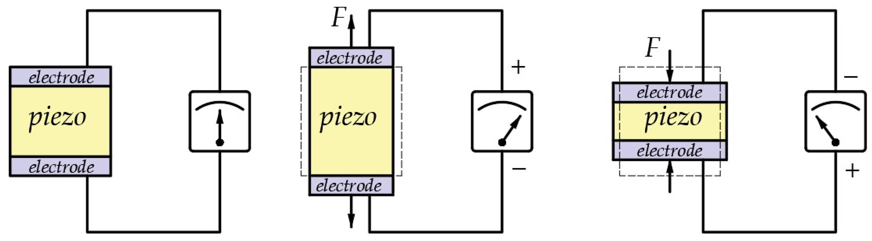
Figure 2.
Inverse piezoelectric effect.
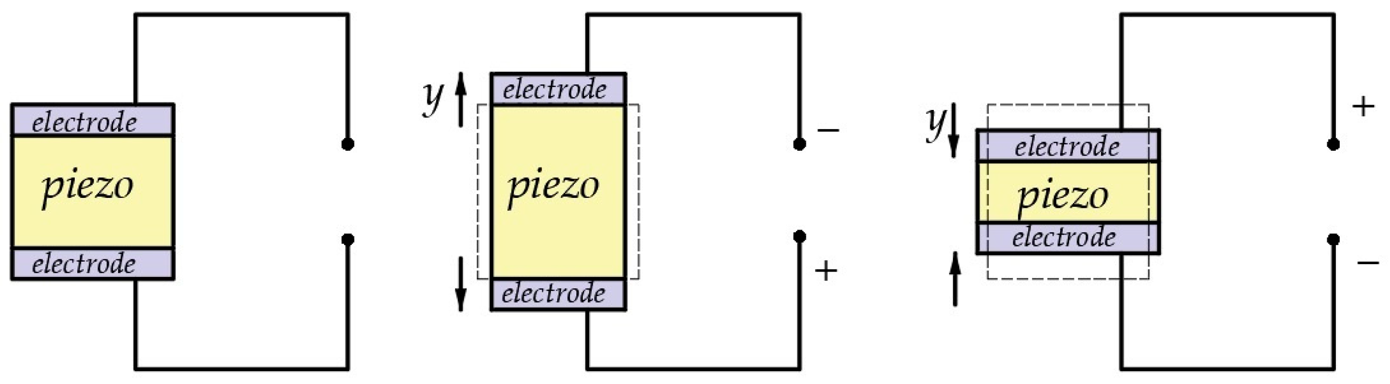
Figure 3.
The crystal structure of BaTiO3 [120].
Figure 3.
The crystal structure of BaTiO3 [120].

Figure 4.
(a) Ferroelectric domains before poling; (b) ferroelectric domains after poling [121].
Figure 4.
(a) Ferroelectric domains before poling; (b) ferroelectric domains after poling [121].

Figure 5.
Piezoelectric hysteresis curve.
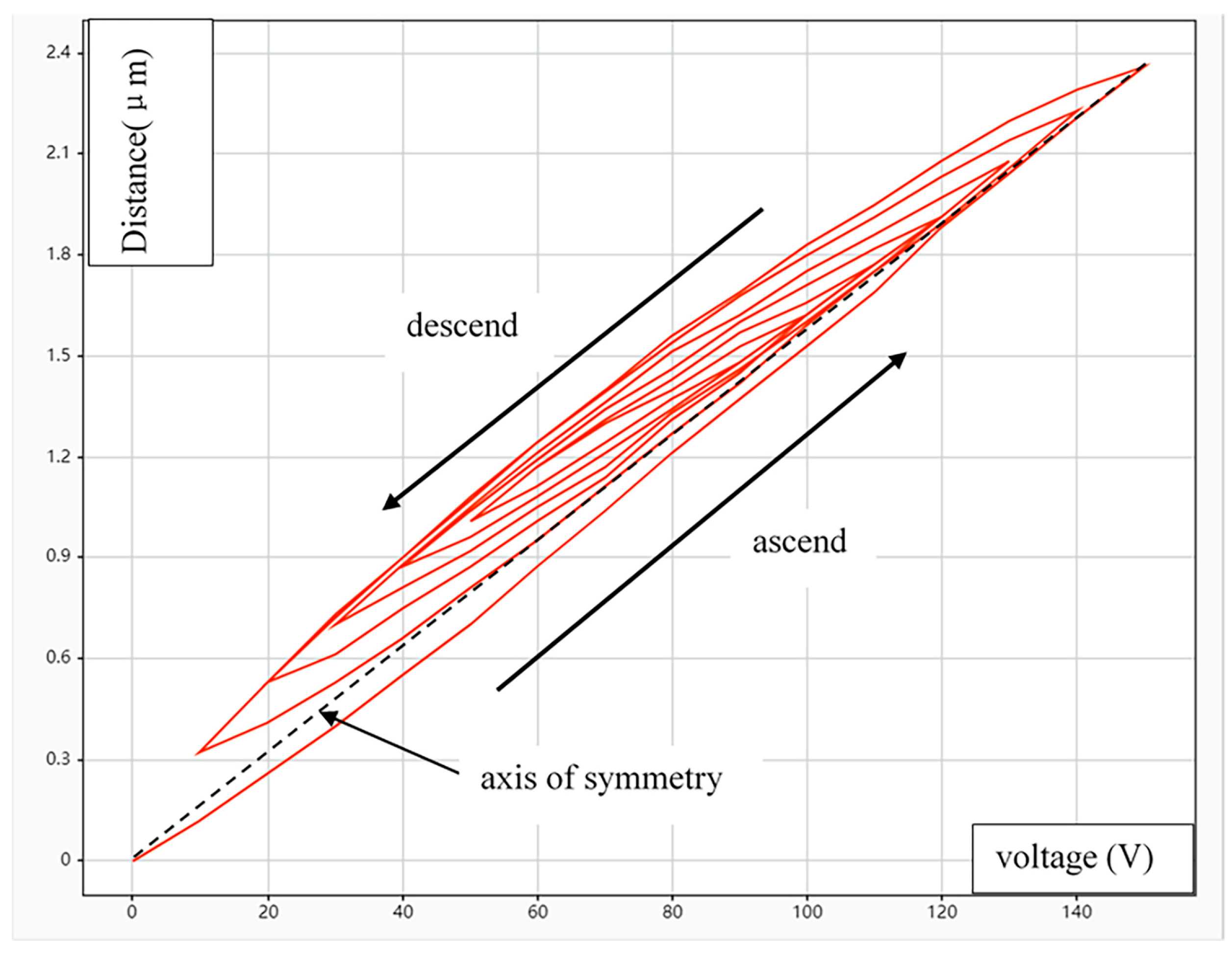
Figure 6.
Piezoelectric hysteresis curves at different temperatures [117].
Figure 6.
Piezoelectric hysteresis curves at different temperatures [117].
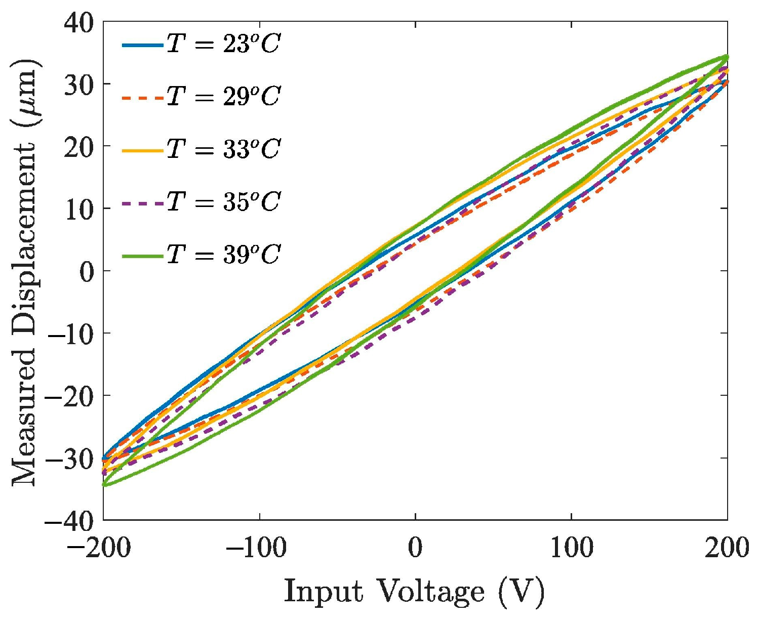
Figure 7.
(a) Piezoelectric hysteresis curves under different loads; (b) piezoelectric hysteresis curves at different voltage frequencies [119].
Figure 7.
(a) Piezoelectric hysteresis curves under different loads; (b) piezoelectric hysteresis curves at different voltage frequencies [119].
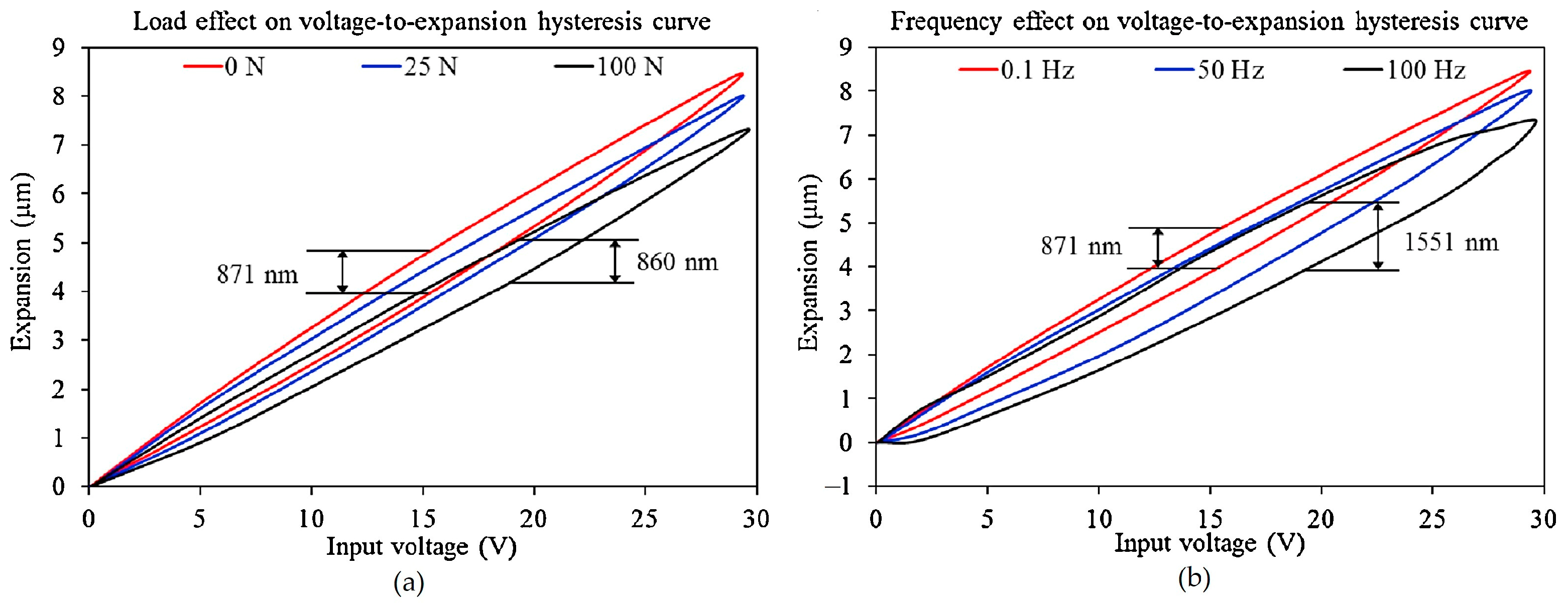
Figure 8.
Inverse model feedforward compensation.

Figure 9.
(a) The input–output relationship diagram of the Relay operator; (b) Preisach model diagram [134].
Figure 9.
(a) The input–output relationship diagram of the Relay operator; (b) Preisach model diagram [134].
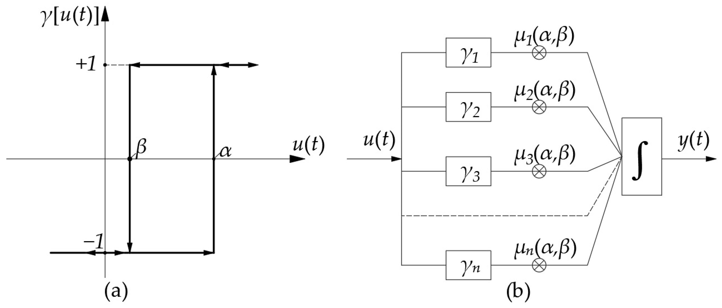
Figure 10.
(a) The integral region of double integrals on the Preisach plane; (b) dividing the integration region based on the relay operator.
Figure 10.
(a) The integral region of double integrals on the Preisach plane; (b) dividing the integration region based on the relay operator.
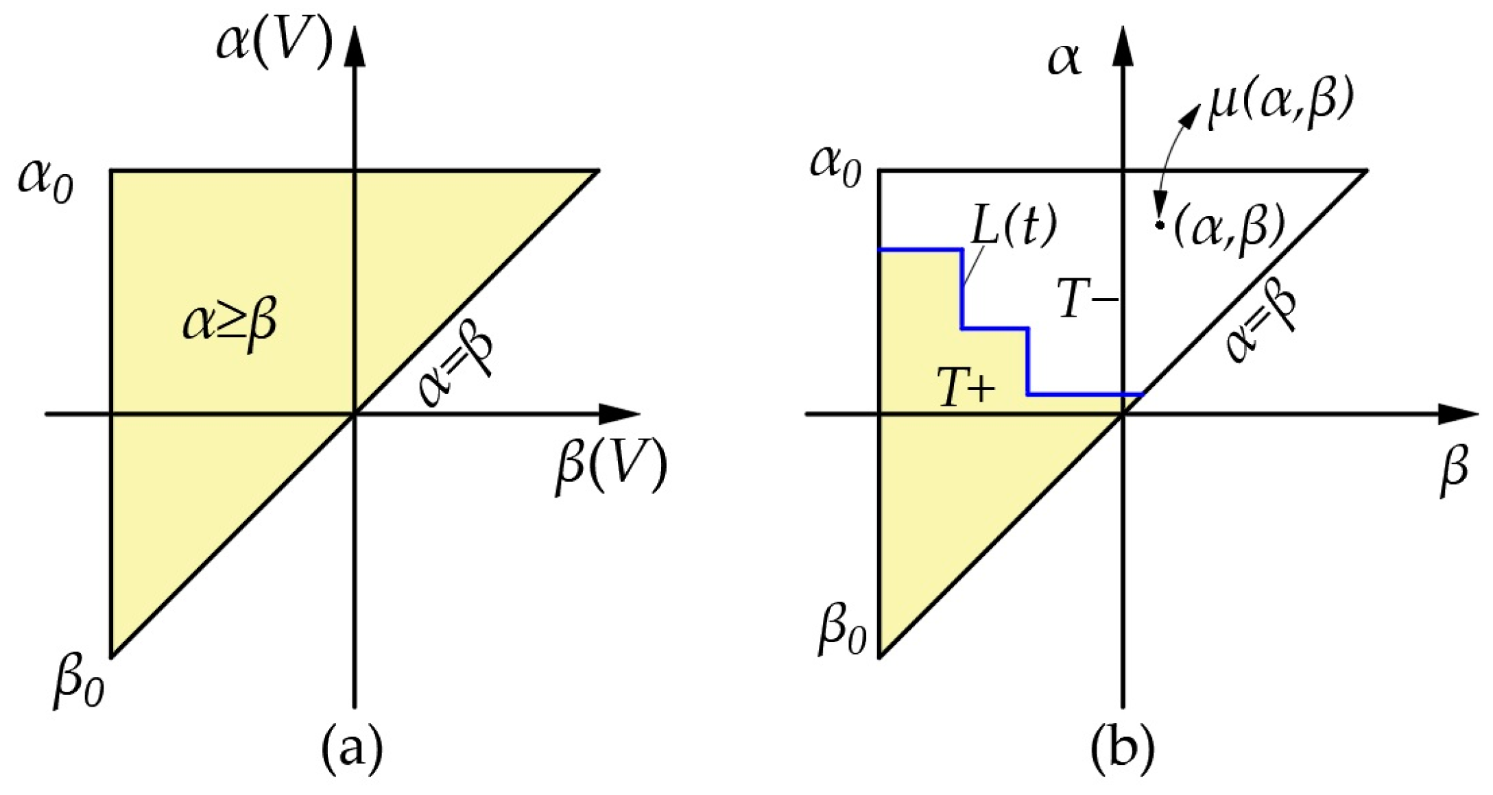
Figure 11.
(a) Voltage–time diagram; (b) displacement–voltage diagram.
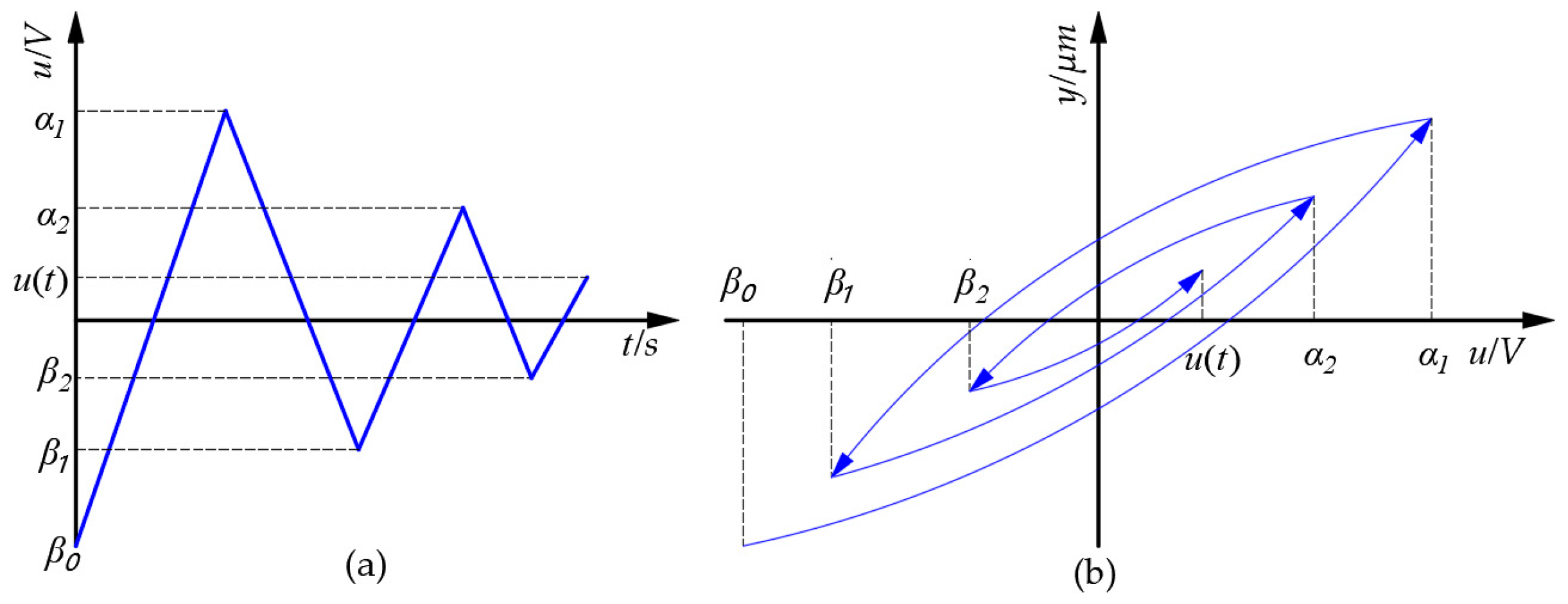
Figure 12.
The variation process of the integration region with voltage: (a) β0 increase to α1; (b) α1 decline to β1; (c) β1 increase to α2; (d) α2 decline to β2; (e) β2 increase to u(t).
Figure 12.
The variation process of the integration region with voltage: (a) β0 increase to α1; (b) α1 decline to β1; (c) β1 increase to α2; (d) α2 decline to β2; (e) β2 increase to u(t).

Figure 13.
(a) y-u diagram; (b) integration region [38].
Figure 13.
(a) y-u diagram; (b) integration region [38].

Figure 14.
Integral region change processes based on the Preisach model of the 1-0 relay operator: (a) β0 increase to α1; (b) α1 decline to β1; (c) β1 increase to α2; (d) α2 decline to β2; (e) β2 increase to u(t).
Figure 14.
Integral region change processes based on the Preisach model of the 1-0 relay operator: (a) β0 increase to α1; (b) α1 decline to β1; (c) β1 increase to α2; (d) α2 decline to β2; (e) β2 increase to u(t).
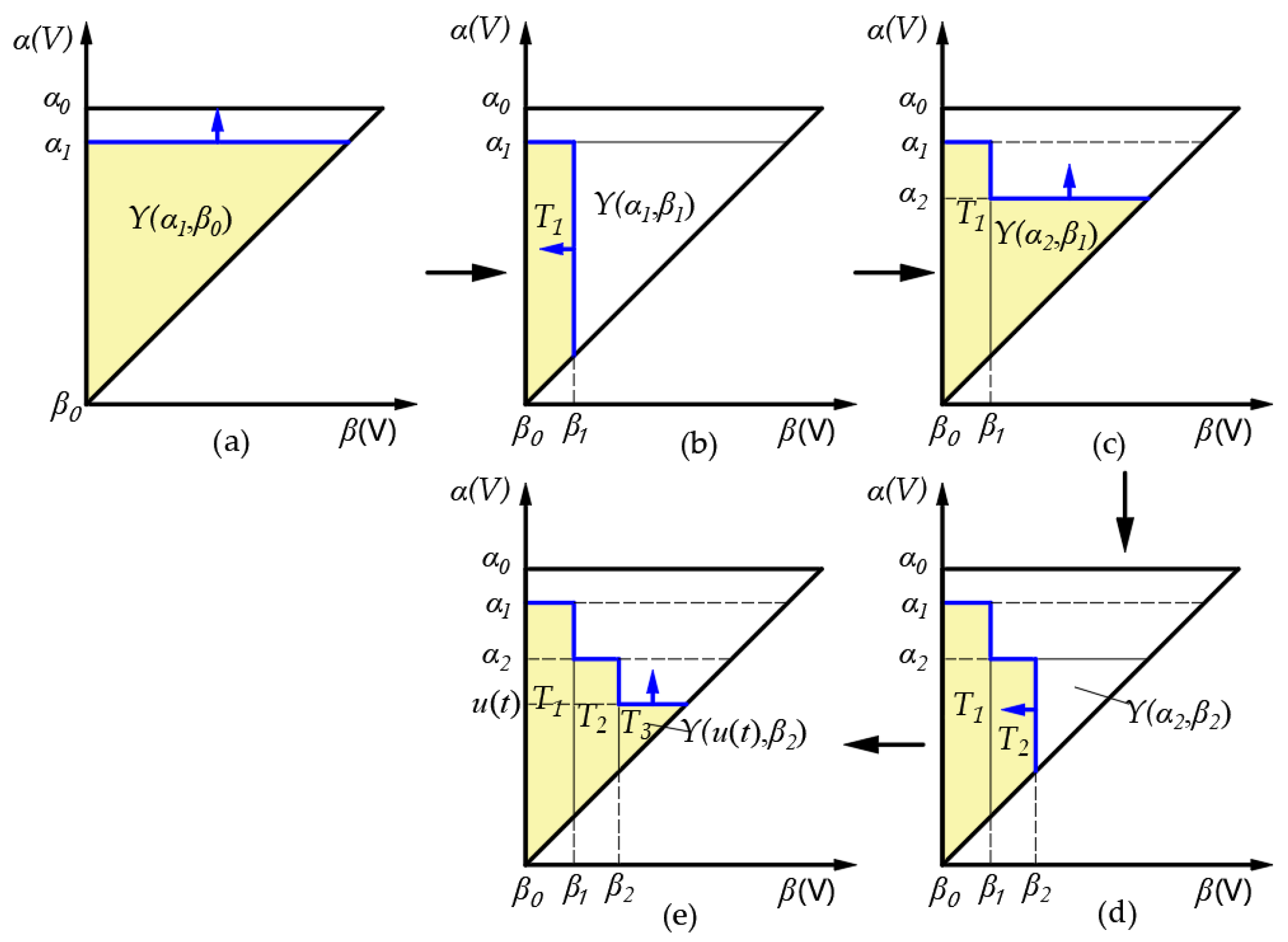
Figure 15.
The value of the Preisach function Y(α,β) (μm) [116].
Figure 15.
The value of the Preisach function Y(α,β) (μm) [116].
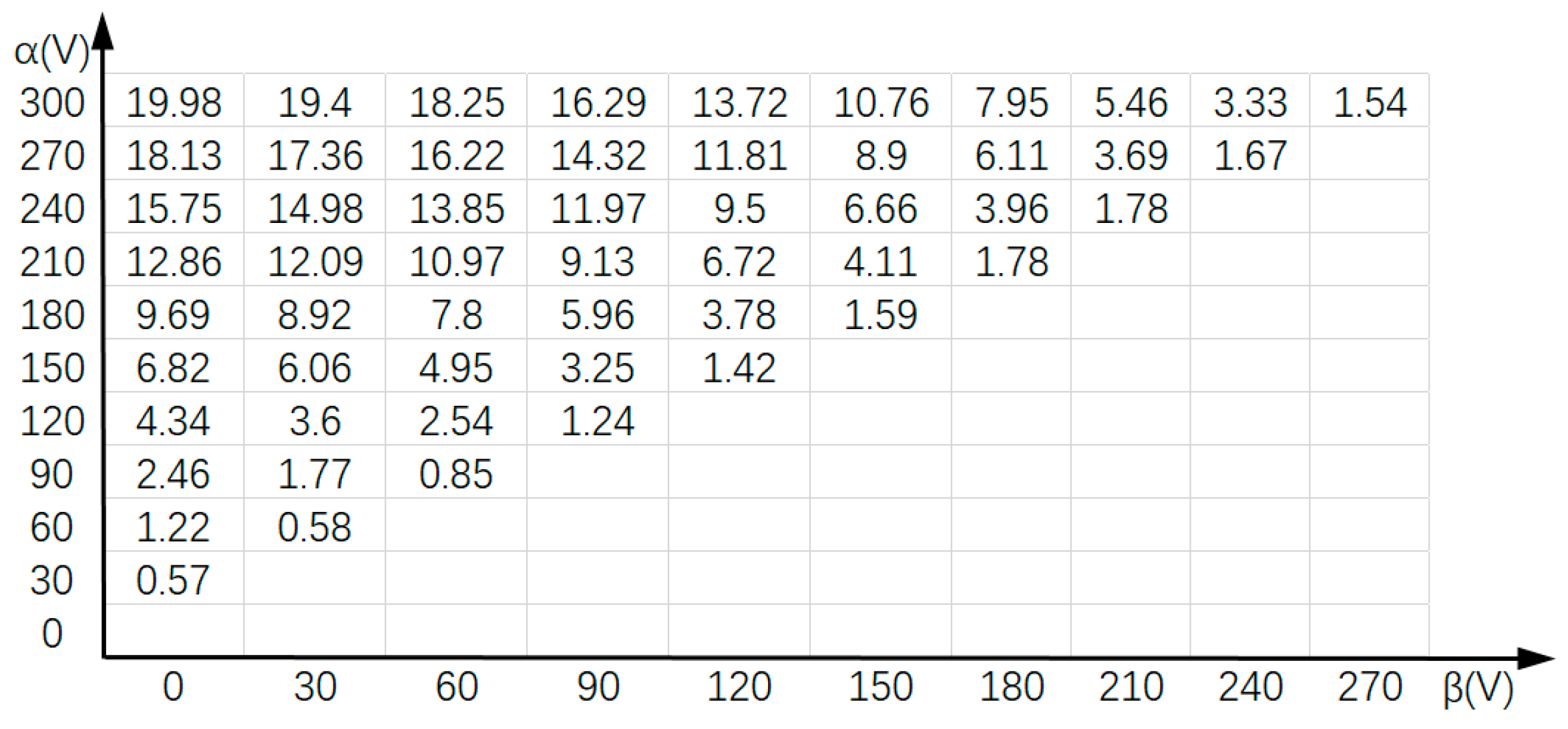
Figure 16.
Principle of inverse model feedforward compensation: (a) an inverse model with a clockwise hysteresis direction; (b) a piezoelectric actuator with a counterclockwise hysteresis direction; (c) the expected displacement yd after compensation is approximately linear with the output displacement y.

Figure 17.
(a) Use two small cars A and B to represent the linear Play operator; (b) the input–output curve of the linear Play operator.
Figure 17.
(a) Use two small cars A and B to represent the linear Play operator; (b) the input–output curve of the linear Play operator.
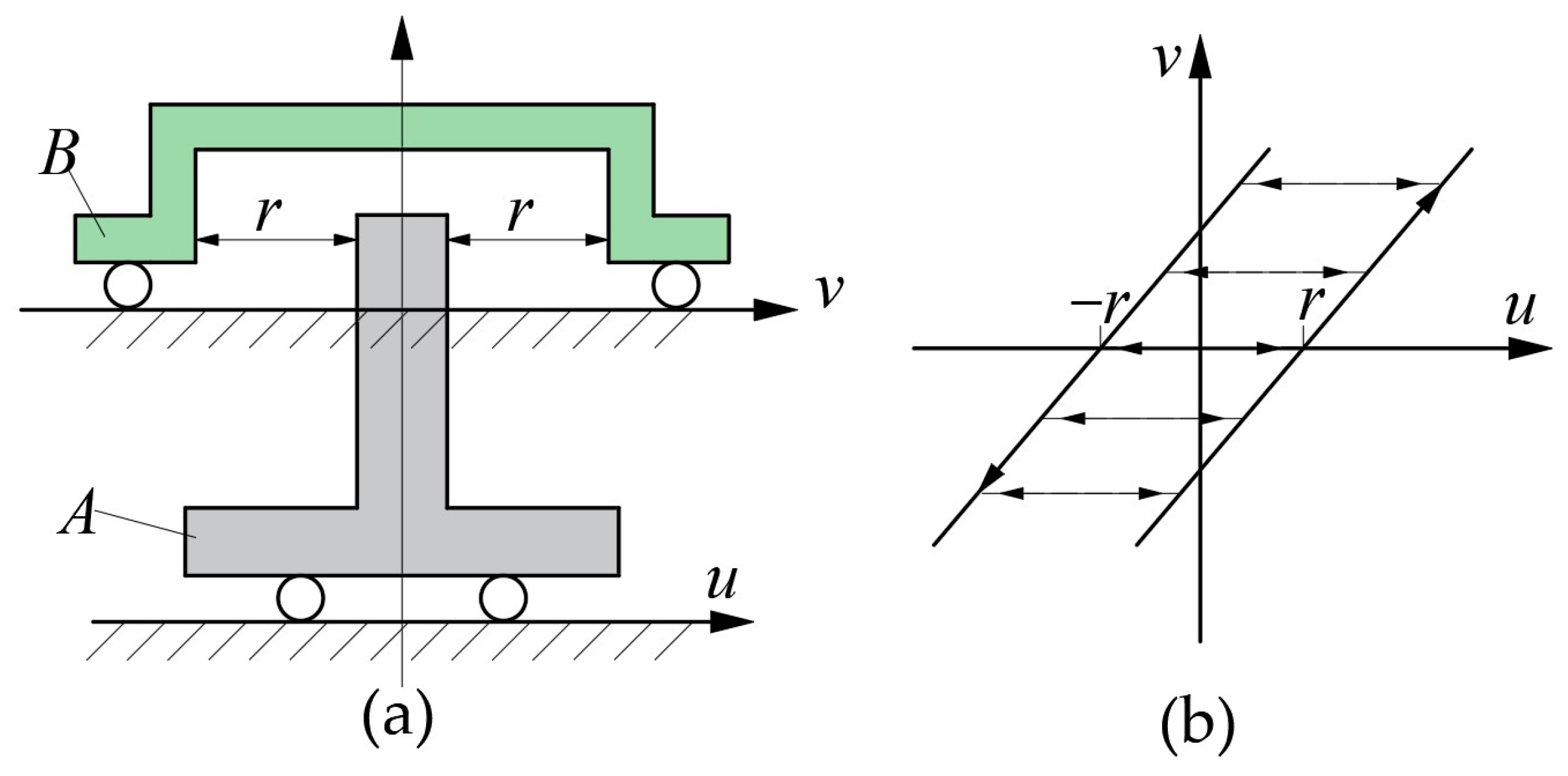
Figure 18.
PI model based on the Play operator.
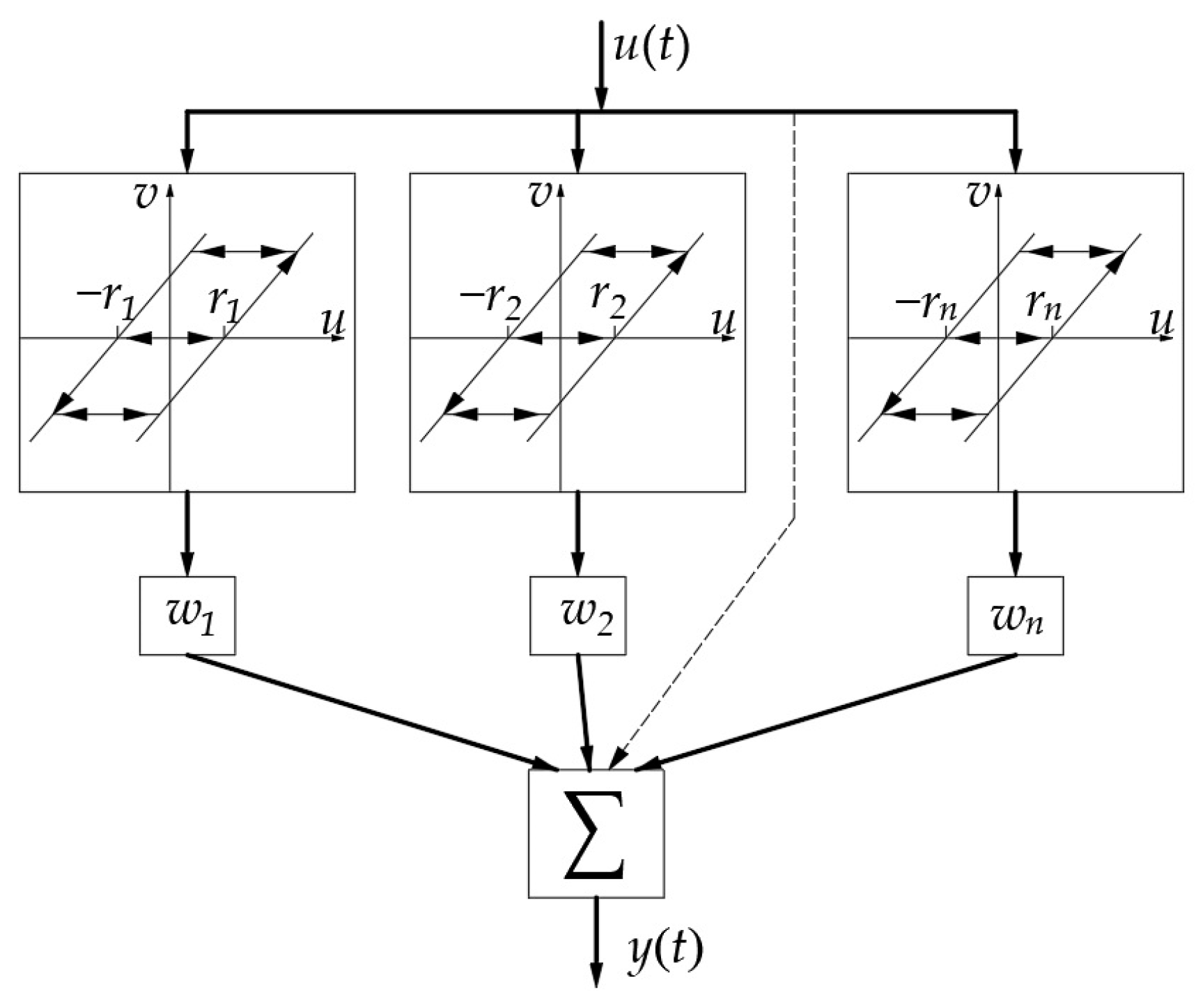
Figure 19.
Schematic diagram of the Play operator superposition.

Figure 20.
Operator weighted superposition composite output displacement.

Figure 21.
(a) Use a spring slider to represent the linear Stop operator; (b) linear Stop operator input–output curve.
Figure 21.
(a) Use a spring slider to represent the linear Stop operator; (b) linear Stop operator input–output curve.
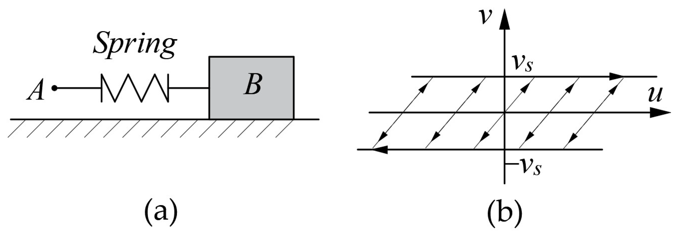
Figure 22.
I/O responses of the (a) Play operator and the (b) Stop operator [116].
Figure 22.
I/O responses of the (a) Play operator and the (b) Stop operator [116].

Figure 23.
I/O relationship of a generalized Play operator [116].
Figure 23.
I/O relationship of a generalized Play operator [116].

Figure 24.
Elasto-Slide element [66].
Figure 24.
Elasto-Slide element [66].
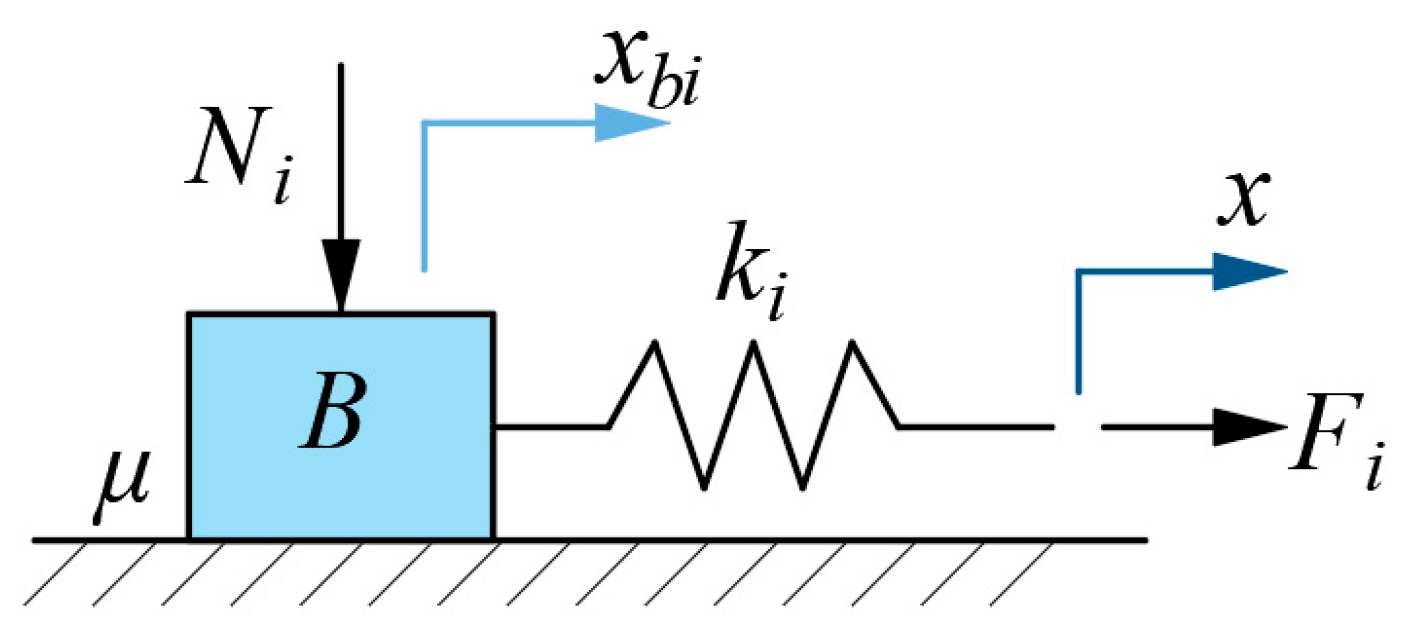
Figure 25.
The input displacement and output force of the massless Elasto-Slide element.
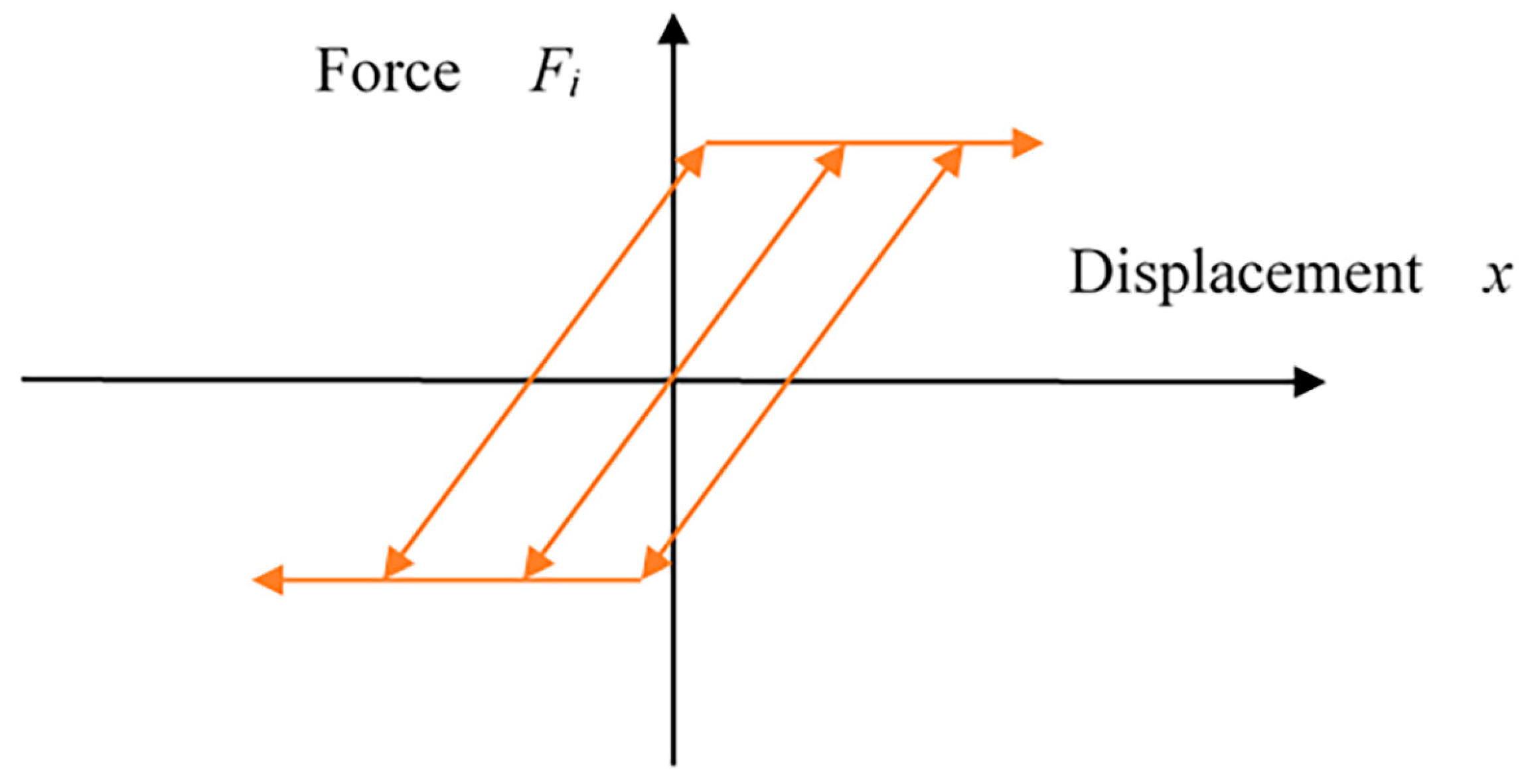
Figure 26.
The generalized Maxwell-Slip model [68].
Figure 26.
The generalized Maxwell-Slip model [68].
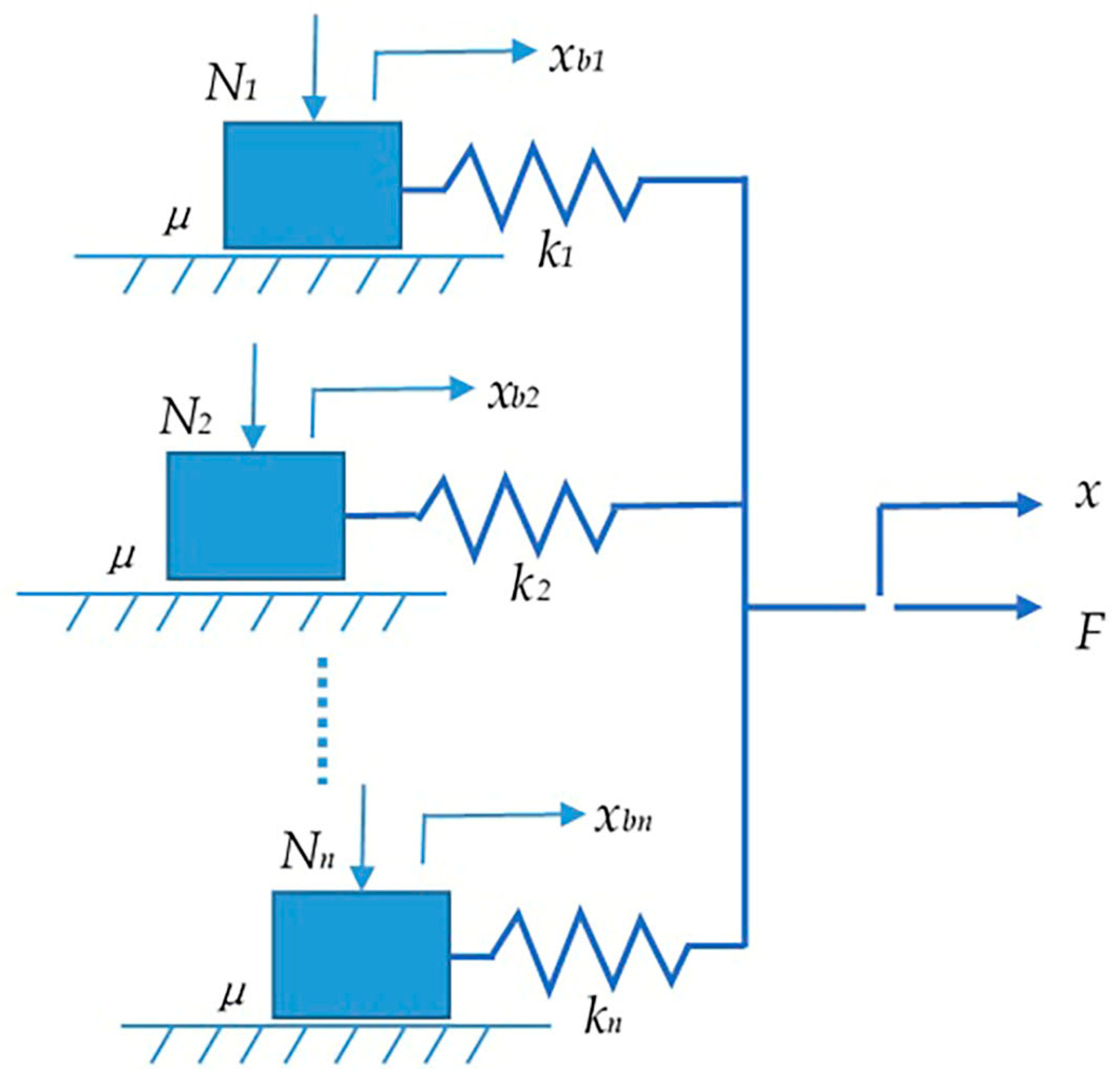
Figure 27.
Maxwell resistive capacitor element.

Figure 28.
Electromechanical model of the piezoelectric ceramic actuator using the MRC module [68].
Figure 28.
Electromechanical model of the piezoelectric ceramic actuator using the MRC module [68].

Figure 29.
Cascading WPMBW Model with a dynamic linear model [99].
Figure 29.
Cascading WPMBW Model with a dynamic linear model [99].

Figure 30.
Schematic diagram of the Inverse WPMBW model [99].
Figure 30.
Schematic diagram of the Inverse WPMBW model [99].

Figure 31.
The structure of the Hammerstein model [111].
Figure 31.
The structure of the Hammerstein model [111].


Table 1.
Comparisons of some basic models *.
| Models | Operator-Based | Differential-Based | |||
|---|---|---|---|---|---|
| Preisach | PI | Maxwell | Duhem | Bouc–Wen | |
| Frequency range(Hz) | ≤32 [39] | ≤100 [61] | ≤100 [68] | ≤100 [87] | ≤120 k [91,96] |
| Inverse model acquisition method | Direct [60] | Direct [57] Indirect [52] | Direct [70] | Direct [84] | Direct [99] |
* Due to the inconsistent evaluation criteria for models in different articles, it is difficult for the data in the table to be very accurate, but they have certain reference value.
Disclaimer/Publisher’s Note: The statements, opinions and data contained in all publications are solely those of the individual author(s) and contributor(s) and not of MDPI and/or the editor(s). MDPI and/or the editor(s) disclaim responsibility for any injury to people or property resulting from any ideas, methods, instructions or products referred to in the content. |
© 2023 by the authors. Licensee MDPI, Basel, Switzerland. This article is an open access article distributed under the terms and conditions of the Creative Commons Attribution (CC BY) license (https://creativecommons.org/licenses/by/4.0/).
Share and Cite
MDPI and ACS Style
Dai, Y.; Li, D.; Wang, D. Review on the Nonlinear Modeling of Hysteresis in Piezoelectric Ceramic Actuators. Actuators 2023, 12, 442. https://doi.org/10.3390/act12120442
AMA Style
Dai Y, Li D, Wang D. Review on the Nonlinear Modeling of Hysteresis in Piezoelectric Ceramic Actuators. Actuators. 2023; 12(12):442. https://doi.org/10.3390/act12120442
Chicago/Turabian StyleDai, Yingli, Dequan Li, and Dong Wang. 2023. "Review on the Nonlinear Modeling of Hysteresis in Piezoelectric Ceramic Actuators" Actuators 12, no. 12: 442. https://doi.org/10.3390/act12120442
Note that from the first issue of 2016, this journal uses article numbers instead of page numbers. See further details here.