
Design of a 2T1R-Type Parallel Mechanism: Performance Analysis and Size Optimization
1
College of Mechanical and Vehicle Engineering, Taiyuan University of Technology, Taiyuan 030024, China
2
Shanxi Province Engineering Technology Research Center for Mine Fluid Control, Taiyuan 030024, China
3
National-Local Joint Engineering Laboratory of Mining Fluid Control, Taiyuan 030024, China
4
School of Mechatronics Engineering, Harbin Institute of Technology, Harbin 150001, China
*
Author to whom correspondence should be addressed.
Actuators 2022, 11(9), 262; https://doi.org/10.3390/act11090262
Submission received: 10 August 2022
/
Revised: 2 September 2022
/
Accepted: 8 September 2022
/
Published: 11 September 2022
(This article belongs to the Section Actuators for Robotics)
Abstract
:The planar three-degree-of-freedom (DoF) parallel mechanism plays a significant role in the fields of automobiles and electronics due to its advantages such as high stiffness, large carrying capability, and stable operation. In this paper, a planar 3-DoF (2T1R) parallel mechanism is derived by structural evolution from the parallelogram by means of Grassmann line geometry and the Atlas method. First, the position equation of the mechanism is established and the inverse kinematics and Jacobian matrix are investigated. The maximum deviation between the theory and simulation results of the inverse kinematics and Jacobian matrix is 0.48%, which verifies the accuracy of the theoretical model. Then, the constraint conditions of the mechanism are defined. Based on the inverse position solution, the numerical method is used to solve the workspace of the mechanism. It is concluded that the ratio of the workspace to the entire triangular space is about 15% higher than that of the 3-PRR parallel mechanism. Next, based on the Jacobian matrix, the performance indexes are established to evaluate stiffness and dexterity. Finally, the size of the mechanism is optimized by means of the genetic algorithm to improve the comprehensive performance.
1. Introduction
Heavy-duty transfer robots have important applications for automotive electronics, ship metal, and dock railway industries, among others. Heavy-duty transfer robots are mainly composed of the robot body, the end-effector, and the root travel mechanism [1,2]. Most heavy-duty transfer robots only have a single-degree-of-freedom rotation mechanism at the root. To increase the transfer range of the robot and improve the stiffness of the mechanism, a planar 3-DOF (2T1R) (T: translational DoF, R: rotational DoF) parallel mechanism is considered for the base of the transfer robot. At present, the design of parallel mechanisms with a large workspace, high precision, high dexterity, and low energy consumption has been in active research. Qu Haibo et al. [3] analyzed a planar 3-DOF parallel mechanism with kinematic redundancy and closed-loop limbs. Furthermore, the workspace of the mechanism was expanded by means of the adjustment of structural redundant branches. Li Xiang et al. [4] studied a single-drive 3-RRR planar parallel mechanism. It was constrained as a single-drive parallel mechanism through a parallelogram to achieve the purpose of easy control and low energy consumption. M. Ganesh et al. [5] classified the shape of the workspace as a function of geometric parameters and proposed an optimization procedure to optimize the workspace of a planar 3-DoF mechanism. This paper aims to design a planar 3-DoF (2T1R) parallel mechanism to realize high stiffness and large carrying capacity.
Type synthesis is a sub-phase of the design phase of the robot. At present, many methods or theories of type synthesis have been proposed, for example, the methods based on topological kinematic chains, Grassmann line geometry and Atlas, the theories based on screws, Lie groups [6,7,8,9], etc. Among them, the Grassmann line geometry and Atlas methods can intuitively analyze the motion and constraints of the mechanism qualitatively. Meanwhile, stiffness and dexterity are also important indicators for analyzing the mechanism. For the performance evaluation of parallel mechanisms, many scholars have presented some standards. For the stiffness of the mechanism, Liu Xinjun et al. [10] regarded the extreme value of the deformation of the end-effector as the stiffness evaluation index. Xu Tianrui et al. [11] took the norm of the robot stiffness matrix under a certain type as the evaluation index. For the dexterity of the mechanism, Zhao Fuqun et al. [12] took the Jacobian condition number as the index of dexterity.
It is also a vital part of the mechanism’s design to optimize the size of the mechanism. Kong Minxiu et al. [13] solved the multi-objective optimization problem based on the NSGA-II algorithm. Zhang Dan et al. [14] optimized the global stiffness of the hybrid mechanism based on the genetic algorithm by taking the rod size as the design variable. Huang Guanyu et al. [15] used the genetic algorithm to perform multi-objective optimization with workspace, stiffness, and dexterity as performance indicators.
In this paper, a planar 3-DOF parallel mechanism is designed by structural evolution from the parallelogram by means of Grassmann line geometry and the Atlas method. The mechanism has the advantages of high rigidity and large carrying capacity. In the same triangular area, the workspace is about 15% larger than that of the 3-PRR mechanism. The mechanism can be envisaged for handling, packaging, etc. In Section 2, the planar 3-DoF (2T1R) mechanism is synthesized. In Section 3, the mechanism description is presented and the DOF is calculated. The kinematic analysis is investigated and the Jacobian matrix is solved in Section 4. Then, the theory and simulation data are compared to verify the correctness of the results. Based on the Jacobian matrix, the workspace, stiffness, and dexterity of the mechanism are analyzed in Section 5. Finally, the sizes of the mechanism are optimized in Section 6.
2. Type Synthesis and Structural Evolution
For the 2T1R-type parallel mechanism with the rotation direction perpendicular to the translation plane, based on Grassmann line geometry and the Atlas method [16], the DoFs and constraints are visually represented by line graphs in Table 1. Based on the generalized Blanding rule [17], the constraint space is a three-dimensional space with a one-dimensional force constraint and a two-dimensional couple constraint. The constraint space of the mechanism is decomposed into three one-dimensional spaces and assigned to three limbs. The specific types of synthesis processes are shown in Table 1. The three limbs can be assigned one-dimensional force constraint and two-dimensional couple constraint, respectively, and each limb can derive a 3-DOF space with two-dimensional translation and one-dimensional rotation. The limb can be realized through branches such as RPR, CR, PRR, etc. (P: prismatic pair; R: revolute pair; and C: cylindrical pair).
It is well known that the motion of each limb in the parallelogram mechanism is equivalent to one translation and one rotation . The kinematic branches obtained by analyzing the DoF space are series branches such as RRR and PRR. Compared to series branches, parallelogram branches have the advantages of strong load-bearing capacity and high stiffness. As shown in Figure 1a, the motion form of a single branch is 1T1R. Inspired by the parallelogram, the motion form of the branch chain in Figure 1a is converted into a parallelogram mechanism. As shown in Figure 1b, a prismatic pair is added to the w-direction of one of the rods of the parallelogram to achieve the same motion form as the branch in Figure 1a. Combined with Figure 1, the equivalence of the two motion forms is proved by the Lie group theory [18]:
where denotes prismatic pair in the direction of the unit vector v; denotes revolute pair with axis vector u and crossing point N. denotes the planar motion of a normal line u, i.e., the two-dimensional motion of a plane and the rotation around the normal line.
In Table 1, the three branched chains have the same DoF space. According to the physical meaning of the line graph, the first two branches of the three branches restrict the two-dimensional rotations in the plane o-xy, and the third branch restricts the translation along the z-axis. Hence, the parallel mechanism can realize two-dimensional translations of the x-axes and y-axes and one-dimensional rotation about the z-axis. During the transportation of the platform, a heavy-duty sensitive ball-type universal wheel [19] is installed at the bottom of the platform, which increases the bearing capacity of the moving platform and enhances the flexibility of transportation.
The mechanism is composed of three limbs. As shown in Table 1, the red line denotes constraint force, the black line denotes rotational DoF and the black line with a double arrow denotes translational DoF. According to Blanding dual line graph rule, the DoF-line graph can be determined when the constraint line graph is known. The corresponding kinematic chain of the mechanism can be identified when the DoF-line graph is given. Note that, neither the decomposition of the constraint-line graph nor the constitution of kinematic chains is unique to the type of synthesis process. In order to increase the transfer range of the platform and ensure the stability of the mechanism, the structural evolution of the PRR branch chain is considered for the first limb and the second limb of the mechanism. Furthermore, the third limb uses a linear drive.
3. Mechanism Description and DoF Calculation
The three limbs can constitute a 3-DOF parallel mechanism as shown in Figure 2a. The simplified diagram of the parallel mechanism is illustrated in Figure 2b. The origin of the static coordinate system is located at O, A1 and A2 are located on the x-axis and A11 is located on the y-axis. The moving platform D1D2D3 is an equilateral triangle. The origin of the moving coordinate system is located at P, the positive direction of tx′-axis is parallel to the direction of the vector D1D2 and D3 is on the y′-axis. The angle formed with the horizontal axis is the rotation angle of the moving platform, C1 is the midpoint of B1B11 and C2 is the midpoint of B2B22. The inclination angle of the frames on both sides of the mechanism is , the value of which is 60°. The following parameters define the details of the simplified schematic diagram:
- l1: the length of the connecting rod A1B1, l2: the length of the vertical rod B1B11, l3: the length of the vertical rod C1D1.
- h1: the moving distance of the prismatic pair A11B11, h2: the moving distance of the prismatic pair A22B22, h3: the moving distance of the prismatic pair A3D3.
- c: the distance from the moving platform P to D1.
- a: the distance of OA1, i.e., the abscissa of A1 in the static coordinate system.
- d: the distance of OA2, i.e., the abscissa of A2 in the static coordinate system.
- e: the abscissa of A3 in the static coordinate system.
- f: the ordinate of A3 in the static coordinate system.
As shown in Figure 2, it is defined that the branch of A1B1D1 is the first branch, the branch of A2B2D2 is the second branch, and the branch of A3D3 is the third branch. In the first branch, the A1B1 rod is the actuating rod, and A1B1B11A11 constitutes a parallelogram linkage, where A11B11 is the prismatic pair. In the second branch, the A2B2 rod is the actuating rod and A2B2B22A22 constitutes a parallelogram linkage, where A22B22 is the prismatic pair. In the third branch, the A3D3 rod is the actuating rod. When the first branch is disassembled alone, there are two degrees of freedom. However, from the analysis of the overall mechanism, the C1D1 rod is restricted by the moving platform. Since the moving distance of the rod A11B11 can be expressed by the rotation angle of A1B1, the actuating link of the first branch is 1. In the whole mechanism, the number of links including the frame is 12, the number of kinematic pairs is 15, and the order of the mechanism is 3.
Therefore, the DoF can be calculated as follows:
where F represents the degree of freedom of the mechanism, λ represents the order of the mechanism, n represents the number of links, g represents the number of kinematic pairs and represents the degrees of the i-th kinematic pair.
4. Kinematics Analysis and Numerical Simulation Verification
4.1. Inverse Kinematics
The inverse position solution is to calculate the rotation angle of the active arm based on the pose of the moving platform. As shown in Figure 2, the output parameters of the mechanism are the position parameters x, and rotation angle of the moving platform. The input parameters are the angle parameters and of the drive pair and the movement parameter of . The key to solving the inverse position solution is to obtain the coordinates of each point of the moving platform D1D2D3. The solution process is as follows:
The origin of the moving coordinate system is located at P, which is denoted as . The rotation matrix of the moving coordinate system relative to the static coordinate system is .
According to the rotation matrix transformation formula, the coordinate of in the moving coordinate system can be denoted as , which can also be expressed as . The coordinate of in the static coordinate system is denoted as , i = 1, 2, 3. Then, the coordinate transformation equation is as follows:
The mathematical model equation of inverse position solution can be obtained by analyzing the geometrical relationship.
Equation (4) is solved and the input parameters φ, and can be expressed as:
where:
4.2. Jacobian Matrix
The Jacobian matrix represents the transmission relationship of the velocity and force between the operating space and the joint space, which is the basis for the performance analysis and evaluation of the parallel mechanism [20].
In the process of solving the inverse position solution, the position constraint equations of first limb, second limb and third limb are obtained. Equation (4) is expressed as:
where the input speed of the driving rod are , and ; the derivation of the output parameters of the moving platform are , and .
Equation (7) is derived from time to obtain the velocity constraint equations as follows:
Therefore, Equation (8) can be guided:
where Ji is denoted as the input-quantity, and Jo is denoted as the output-quantity, ; and .
Hence, the Jacobian matrix of the mechanism is the following:
4.3. The Verification of Inverse Kinematics and Jacobian Matrix
The correctness of the inverse kinematics and the Jacobian matrix is verified by the ADAMS dynamic simulation software. The trajectory equations are the coordinates of the point in the moving platform and the angle of rotation around the z-axis. The trajectory equations of the moving platform are as follows:
where t represents the duration of the movement (the unit is second).
The simulation model of the mechanism in ADAMS software is presented in Figure 3. In the first limb, A1, A11, B1, B11 and D1 are set as revolute joints and h1 is set as a prismatic joint. In the second limb, A2, A22, B2, B22 and D2 are set as revolute joints and h2 is set as the prismatic joint. In the third limb, A3 and D3 are set as revolute joints and h3 is set as the prismatic joint. To ensure the uniqueness of the solution, the center P of the moving platform is set to the revolute joint. The elementary parameters for each component of the mechanism are given in Table 2.
The comparisons between the theory and simulation results of inverse kinematics are shown in Figure 4, and the comparisons between the theory and simulation results of the input velocity of the rods are shown in Figure 5. The solver of the ADAMS software establishes the dynamic equation of the mechanical system through Lagrange’s equation of the first kind. The result of its solution is accurate.
In the process of verifying the inverse kinematics, due to the counterclockwise rotation of the moving platform, the motion amplitude of the first branch of the mechanism is greater than that of the second and third branches, resulting the larger errors in Figure 4a than those in Figure 4b,c. It can be concluded that the theoretical data obtained from the inverse kinematics solution and the Jacobian matrix of the mechanism are basically consistent with the simulation data, and the maximum deviation is 0.48%. Thus, the correctness of the results is verified, which provides a theoretical basis for the subsequent solution of the workspace and the performance analysis of the mechanism.
5. Performance Analysis
5.1. Workspace
- (1)
- Constraint
The workspace of the mechanism is the working area that the end-effector can reach. It is an important basis for evaluating the performance of the mechanism. In this paper, the workspace is considered as the maximum active range of the center P point of the end-effector. The main constraints that restrict the workspace include link length constraint, the constraint of the angle of actuating rod, travel constraint of the prismatic pair, the interference of adjacent rods, etc. The above constraints are defined as follows:
- (a)
- Constraint of link-length
- (b)
- Constraint of the angle of actuating rod
In the simplified diagram of the parallel mechanism, the actuating rods of the revolute pair are the rod A1B1 and the rod A2B2. Due to the existence of the prismatic pair A11B11 and A22B22, the rotation angles of the revolute pair are limited. Due to the differences between the length of the rod and the position of the frame, the rotation angles of the revolute pair are also different. Let the maximum rotation angles of the revolute pair be and , and let the minimum rotation angles be and . Then, the constraint conditions of rotation angle are
- (c)
- Travel constraint of the prismatic pair
The travel of the prismatic pairs is also an important factor to restrict the workspace of the mechanism. Among them, let the maximum displacement of the prismatic pair A3D3 and the auxiliary prismatic pairs A11B11 and A22B22 be , and let the minimum displacement be . Then, the travel constraints of the prismatic pair are:
- (d)
- The interference of adjacent rods
Since the moving platform and frame are connected by connecting rods, and there may be some interference between the connecting rods when the mechanism works. Let
where is the shortest distance between two adjacent rods; is the diameter of the cylindrical rod.
The numerical method is used to solve the workspace of the parallel mechanism [21]. According to the extreme value theory and optimization method, as many joint variables as possible are selected, and the inverse position solution and the constraint conditions between the rods are defined. The position coordinates of as many output points as possible are obtained by MATLAB. The coordinate points form the workspace of the parallel mechanism. The more coordinates are solved, the better the workspace of the mechanism can be reflected.
The workspace of the end-effector is shown in Figure 6, and the relevant data obtained in the diagram are shown in Table 3. The boundaries of the workspace are x [177.75 mm, 341.22 mm], y [−6.51 mm, 201.37 mm]. By analyzing the data in Figure 6, it can be concluded that the workspace of the mechanism is symmetrical about x = 260 mm, and the value of the y-coordinate largely depends on the range of the prismatic pair h3. It can be further concluded that the workspace area of the mechanism accounts for 28% of the whole triangle area, which meets the transport requirements of the transport platform.
- (2)
- Comparison to 3-PRR workspace
Due to the different rod sizes and frame positions of the mechanism, the comparisons of the workspace are also different. The method used in this paper to compare the workspace is the proportion method, that is, the ratio of the workspace obtained by the mechanism to the space occupied by the entire mechanism. The optimized workspace obtained by the 3-PRR mechanism accounts for about 13% of the entire area [22], while the workspace of the mechanism accounts for 28% of the entire area. It is noted that the workspace performance of the mechanism can be further improved after the optimized design.
5.2. Stiffness Modeling
When the force F0 acts on the moving platform, the maximum deformation of the moving platform can be used as an index to evaluate stiffness [10]. The stiffness of the parallel mechanism mainly relies on the following factors, such as the length and material of the rods, the orientation and position of the moving platform, etc.
It is supposed that the stiffness of the i-th chain is expressed as ki. Hence, the relationship between the joint torque and the deformation of the branch chain is
where is the joint torque and is the deformation of the branched chain.
Equation (16) is derived in matrix form as:
where is the deflection of the force transmission system, is the spring matrix of the mechanism, , = ,.
The relationship between and is
where is the deflection of the moving platform.
Based on the duality of kinematics and statics, the forces and moments applied at the end-effector under static conditions are related to the forces or moments required at the actuators to maintain the equilibrium by transposing the Jacobian matrix J [23]. Then
Combining Equations (17)–(19) guides to:
where is the stiffness matrix.
To obtain the maximum value of terminal deformation, the Lagrange function is constructed.
where is the Lagrangian multiplier.
The conditions for the conditional extremum are:
Then:
From Equation (23), is the eigenvalue of .
Therefore, the following equation can be guided:
From Equation (24), the limit value of is equal to the maximum or minimum eigenvalue of . Let be the unit matrix and , then:
When the moving platform of the mechanism rotates at 10°, the distribution of local stiffness index (LSI) in the workspace is shown in Figure 7. The ranges of the x-axis and y-axis are (195, 265) and (80, 190), respectively. The minimum deformation value in the workspace is taken as the evaluation index. The smaller the minimum deformation of a mechanism, the better the stiffness performance. When the singular value of the mechanism is removed, it can be obtained that the maximum value of is 0.09, which is smaller than 0.14 for 3-RRR and 0.35 for 2-RRR [23]. Therefore, the stiffness of the mechanism is higher than that of the 2-RRR mechanism and the 3-RRR mechanism.
It can be concluded from Figure 7 that the maximum stiffness is near (240, 170) and the minimum stiffness is in the workspace area. Two high points appear near (240, 170) and (215, 40), while the value tends to be stable in other areas. The reason is that when the two links l1 and l2 are in the collinear position (that is, the singular position of the mechanism), the stiffness of the mechanism tends to be infinite. Compared to the singular positions of the first type of the 3-RRR mechanism [24], it can be found that it is similar to the positions of the highest stiffness in this paper. The stiffness increases rapidly when the mechanism is singular. In addition, the analysis of stiffness provides a basis for the parameter design, working area selection and stiffness control of the mechanism.
5.3. Dexterity Analysis
At present, there are two main indexes for measuring robot dexterity: one is the Jacobian condition number, and the other is manipulability. The manipulability can directly identify the type of singularity, but it has defects in the evaluation of the dexterity index [25]. In this paper, the Jacobian condition number is used to evaluate the dexterity of the parallel mechanism.
The Jacobian condition number can be calculated by means of spectrum norm as follows:
where .
Square both sides of Equation (26) and then
Therefore, the maximum singular value of matrix is the spectrum norm of matrix J, which is expressed as . Similarly, the reciprocal of the minimum singular value of matrix is the spectrum norm of , which is expressed as . Then
To understand the dexterity values of the mechanism in the workspace, when the end-effector rotates at 30°, the local dexterity index distribution in the workspace is shown in Figure 8. The ranges of the x-axis and y-axis in Figure 8 are [200, 260] and [60, 145], respectively. The value of ranges from approximately 0 to 1, and the higher the value, the better the overall kinematic performance of the mechanism in the workspace. In Figure 8, the maximum and minimum dexterity values in the workspace are 0.91 and 0.16. The dexterity values are mostly in the range of 0.3~0.65.
As shown in Figure 8, the value of in the dark purple area is small and the kinematics performance is slightly poor. The reason is that the first limb and the second limb of the mechanism adopt a parallelogram structure. The shorter side of the parallelogram is relatively close to the edge of the workspace, which limits the activity space of the mechanism. Therefore, the value of here is small and the kinematics performance is slightly worse. The kinematics performance of the mechanism can be further improved after optimized design.
6. Size Optimization
6.1. Evaluation Standard
The essence of optimization is to adjust the geometric dimensions of the mechanism in order to achieve better performance [15]. In order to evaluate the characteristics of the mechanism, a comprehensive evaluation standard is proposed.
The mechanism’s workspace is the result of the superposition of each discrete point. The workspace can be measured by the area composed of the obtained points. Therefore, the workspace (W) is defined as:
For the mechanism’s stiffness, the concept of global stiffness index (GSI) [26] is proposed. The GSI refers to the average stiffness of points in the workspace, which is denoted as follows:
The mechanism’s dexterity is also an effective factor that involves the performance of the mechanism. The global dexterity index (GDI) can be used as an index to evaluate dexterity, which is defined as the average dexterity in the workspace. Hence, it can be expressed as:
Based on the above criteria, the size parameters of the parallel mechanism are optimized to obtain optimal performance. It is required to maximize the workspace on the premise of better dexterity and stiffness performance of the mechanism.
6.2. Optimization Process
The genetic algorithm (GA) draws on Darwin’s theory of evolution and Mendel’s theory of genetics, which simulates the process of inheritance and evolution of organisms in the natural environment, and forms an adaptive global optimization search algorithm. It has the advantages of good convergence and robustness [27].
The genetic algorithm is utilized to optimize the size of the parallel mechanism. In the optimization process, the optimization variables are , , , . The variable constraints are shown in Table 4. Then, the optimization parameters are set as follows: population = 30, crossover probability = 0.8, mutation probability = 0.05, evolutional generation = 300. The optimization results of the optimized design variables are shown in Table 5. Furthermore, Table 6 shows the 30 sets of objective functions. Furthermore, the orders of the relevant objective function values are consistent with the orders of the optimization design variables.
In order to select the best size scheme, a comprehensive index is proposed to evaluate 30 groups of design variables. According to the data, GSI is mostly in the scale, GDI is in the scale, and the workspace is in the scale. Therefore, the appropriate weights can be selected to reflect the overall performance of the mechanism, so the objective function value is
where the weights of different objective functions are defined . By comparing the objective function values in Table 6, it can be concluded that the sixth group of solutions is the optimal solution. In the sixth group of data, the corresponding workspace of the mechanism is 4443.18, the stiffness is 5.72, and the dexterity is 0.88. It is concluded that the performance of the optimized mechanism is improved. Furthermore, the sixth group of convergence diagrams based on the optimization process is shown in Figure 9.
7. Conclusions
- (1)
- A planar 3-DoF (2T1R) parallel mechanism is derived by structural evolution from the parallelogram by means of Grassmann line geometry and the Atlas method. The key property of the mechanism is that the two branches are designed as parallel closed-loop structures. The overall mechanism has the characteristics of high stiffness and large carrying capacity.
- (2)
- The position equation of the mechanism is established and the inverse kinematics and Jacobian matrix are investigated. The maximum deviation between the theory and simulation results of the inverse kinematics and Jacobian matrix is 0.48%, which verifies the accuracy of the theoretical model. Based on the results of inverse kinematics, the workspaces of the mechanism can be produced. The ratio of the workspace to the entire triangle space is about 15% higher than that of the 3-PRR parallel mechanism.
- (3)
- Based on the Jacobian matrix, the performance indexes are established to evaluate the stiffness and dexterity of the mechanism. Finally, the genetic algorithm is used to optimize the size of the rods to improve the comprehensive performance of the mechanism.
In addition, future work will focus on the position deployment of the frame and the branches, the singularity of the mechanism and the development of the prototype to enhance the practicability of the research.
Author Contributions
Conceptualization, D.W. and J.Z.; Data curation, H.G. and R.L.; Funding acquisition, J.Z.; Project administration, J.Z.; Software, Z.K.; Supervision, J.Z.; Writing—Original draft, D.W.; Writing—review and editing, D.W. and J.Z. All authors have read and agreed to the published version of the manuscript.
Funding
This research was funded by National Key R&D Program of China (Project No. 2018YFB1307900), National Natural Science Foundation of China (Project No. 51835002), Natural Science Foundation of Shanxi Province (Project No. 201901D211010) and Technology Innovation Foundation of Shanxi University (Project No. 2019L0177).
Institutional Review Board Statement
Not applicable.
Informed Consent Statement
Not applicable.
Data Availability Statement
Not applicable.
Acknowledgments
The authors would like to thank Taiyuan University of Technology and Harbin Institute of Technology for their support. The authors are sincerely grateful to the reviewers for their valuable review comments, which substantially improved the paper.
Conflicts of Interest
The authors declare no conflict of interest.
References
- Zhang, Q.X.; Chen, W.H. A review of the research progress of heavy-duty handling robots. Sci. Technol. Innov. 2021, 100–101, 105. [Google Scholar]
- Jin, X.; Fang, Y.; Zhang, D.; Gong, J. Design of dexterous hands based on parallel finger structures. Mech. Mach. Theory 2020, 152, 103952. [Google Scholar] [CrossRef]
- Qu, H.; Hu, L.; Guo, S.; Li, S. Statics analysis of a planar parallel mechanism with kinematic redundancy and closed-loop limb. J. Cent. South Univ. (Sci. Technol.) 2020, 51, 2758–2771. [Google Scholar]
- Li, X.; Li, R.Q.; Li, H.; Ning, F.P. A numerical solution of coupler curve and orientation for reconfigurable single-driven 3-RRR planar parallel mechanism. Acta Armamentarii 2021, 42, 1074–1082. [Google Scholar]
- Ganesh, M.; Bihari, B.; Rathore, V.S.; Kumar, D.; Kumar, C.; Sree, A.R.; Sowmya, K.N.; Dash, A. Determination of the closed-form workspace area expression and dimensional optimization of planar parallel manipulators. Robotica 2017, 35, 2056–2075. [Google Scholar] [CrossRef]
- Yang, H.; Guo, H.; Wang, Y.; Liu, R.; Deng, Z. Configuration synthesis of planar folded and common overconstrained spatial rectangular pyramid deployable truss units. Chin. J. Aeronaut. 2019, 32, 1772–1787. [Google Scholar] [CrossRef]
- Liu, W.; Liu, H. Synthesis of asymmetric parallel mechanism with multiple 3-DOF motion modes. Adv. Mech. Eng. 2022, 14. [Google Scholar] [CrossRef]
- Li, L.; Fang, Y.; Yao, J.; Wang, L. Type synthesis of a family of novel parallel leg mechanisms driven by a 3-DOF drive system. Mech. Mach. Theory 2022, 167, 104572. [Google Scholar] [CrossRef]
- Xie, F.; Li, T.; Liu, X. Type synthesis of 4-DOF parallel kinematic mechanisms based on Grassmann line geometry and Atlas method. Chin. J. Mech. Eng. 2013, 26, 1073–1081. [Google Scholar] [CrossRef]
- Liu, X.J. The Relationships between the Performance Criteria and Link Lengths of the Parallel Manipulators and Their Design Theory. Ph.D. Thesis, Yanshan University, Qinhuangdao, China, 1999. [Google Scholar]
- Xu, T.; Wu, J.; Zhang, B. Optimization design of a novel 4-DOF parallel manipulator. In Proceedings of the 2019 IEEE 9th Annual International Conference on CYBER Technology in Automation, Control, and Intelligent Systems (CYBER), Suzhou, China, 29 July–2 August 2019; pp. 963–968. [Google Scholar]
- Zhao, F.Q.; Guo, S.; Xu, Z.C.; Dian, L. Design and analysis of high performance machine tool based on redundant parallel mechanism. J. Cent. South Univ. (Sci. Technol.) 2019, 50, 67–74. [Google Scholar]
- Kong, M.; Chen, L.; Du, Z.; Sun, L. Multi-objective optimization on dynamic performance for a planar parallel mechanism with NSGA-II Algorithm. Robot 2010, 32, 271–277. [Google Scholar] [CrossRef]
- Zhang, D.; Wei, B. Stiffness Analysis and Optimization for a Bio-Inspired 3-DOF Hybrid Manipulator; Springer International Publishing: Berlin/Heidelberg, Germany, 2017. [Google Scholar]
- Huang, G.; Guo, S.; Zhang, D.; Qu, H.; Tang, H. Kinematic analysis and multi-objective optimization of a new reconfigurable parallel mechanism with high stiffness. Robotica 2017, 36, 1–17. [Google Scholar] [CrossRef]
- Xie, F.; Liu, X.J.; Wang, C. Design of a novel 3-DoF parallel kinematic mechanism: Type synthesis and kinematic optimization. Robotica 2015, 33, 622–637. [Google Scholar] [CrossRef]
- Yu, J.; Li, S.; Su, H.-J.; Culpepper, M.L. Screw theory based methodology for the deterministic type synthesis of flexure mechanisms. ASME.J. Mech. Robotics. 2011, 3, 031008. [Google Scholar] [CrossRef]
- Liang, D.; Zhang, Z.J.; Chang, B.Y. A novel SCARA parallel mechanism with double parallelogram branches. Trans. Chin. Soc. Agric. Mach. 2022, 53, 422–434. [Google Scholar]
- Li, Y.Q. A Heavy-Duty Sensitive Ball-Type Universal Wheel. CN202011232266.0, 5 February 2021. [Google Scholar]
- Zhao, Y.Z.; Cao, Y.C.; Liang, B.W.; Zhao, T.S. Determination and synthesis of translational parallel mechanism with constant Jacobian Matrix. J. Mech. Eng. 2017, 53, 101. [Google Scholar] [CrossRef]
- Agheli, M.; Nestinger, S.S. Comprehensive closed-form solution for the reachable workspace of 2-RPR planar parallel mechanisms. Mech. Mach. Theory 2014, 74, 102–116. [Google Scholar] [CrossRef]
- Min, S.; Hong, Y.L.; Dong, J.-J.L. Workspace and dexterity optimization of 3-PRR planar parallel manipulator. In Proceedings of the 12th International Conference of European Society for Precision Engineering and Nanotechnology, Stocholm, Sweden, 4 June 2012; pp. 360–363. [Google Scholar]
- Wu, J.; Wang, R.; Wang, R. A comparison study of two planar 2-DOF parallel mechanisms: One with 2-RRR and the other with 3-RRR structures. Robotica 2010, 28, 937–942. [Google Scholar] [CrossRef]
- Rybak, L.A.; Gaponenko, E.V.; Malyshev, D.I.; Behera, L. Determination of the working area and singularity zones of the 3-RRR robot based on the non-uniform coverings’ method. J. Phys. Conf. Ser. 2019, 1353, 012057. [Google Scholar] [CrossRef]
- Yu, J.J.; Liu, X.J.; Ding, X.L.; Dai, J.S. Foundation of Mathematics of Robot Mechanism, 2nd ed.; China Machine Press: Beijing, China, 2008; pp. 203–219. [Google Scholar]
- Gao, Z.; Zhang, D. Performance analysis, mapping, and multi-objective optimization of a hybrid robotic machine tool. Ind. Electron. IEEE Trans. 2015, 62, 423–433. [Google Scholar] [CrossRef]
- Zhang, C.; Wang, C.; Miao, Q. Two-Stage optimization of a reconfigurable asymmetric 6-DOF haptic robot for task-specific workspace. In Proceedings of the 2021 IEEE/RSJ International Conference on Intelligent Robots and Systems (IROS), Prague, Czech Republic, 27 September 2021–1 October 2021; pp. 8345–8351. [Google Scholar]
Figure 1.
Configuration evolution (a) single-branch PR mechanism (b) RR-RPR mechanism with parallelogram branches.
Figure 1.
Configuration evolution (a) single-branch PR mechanism (b) RR-RPR mechanism with parallelogram branches.
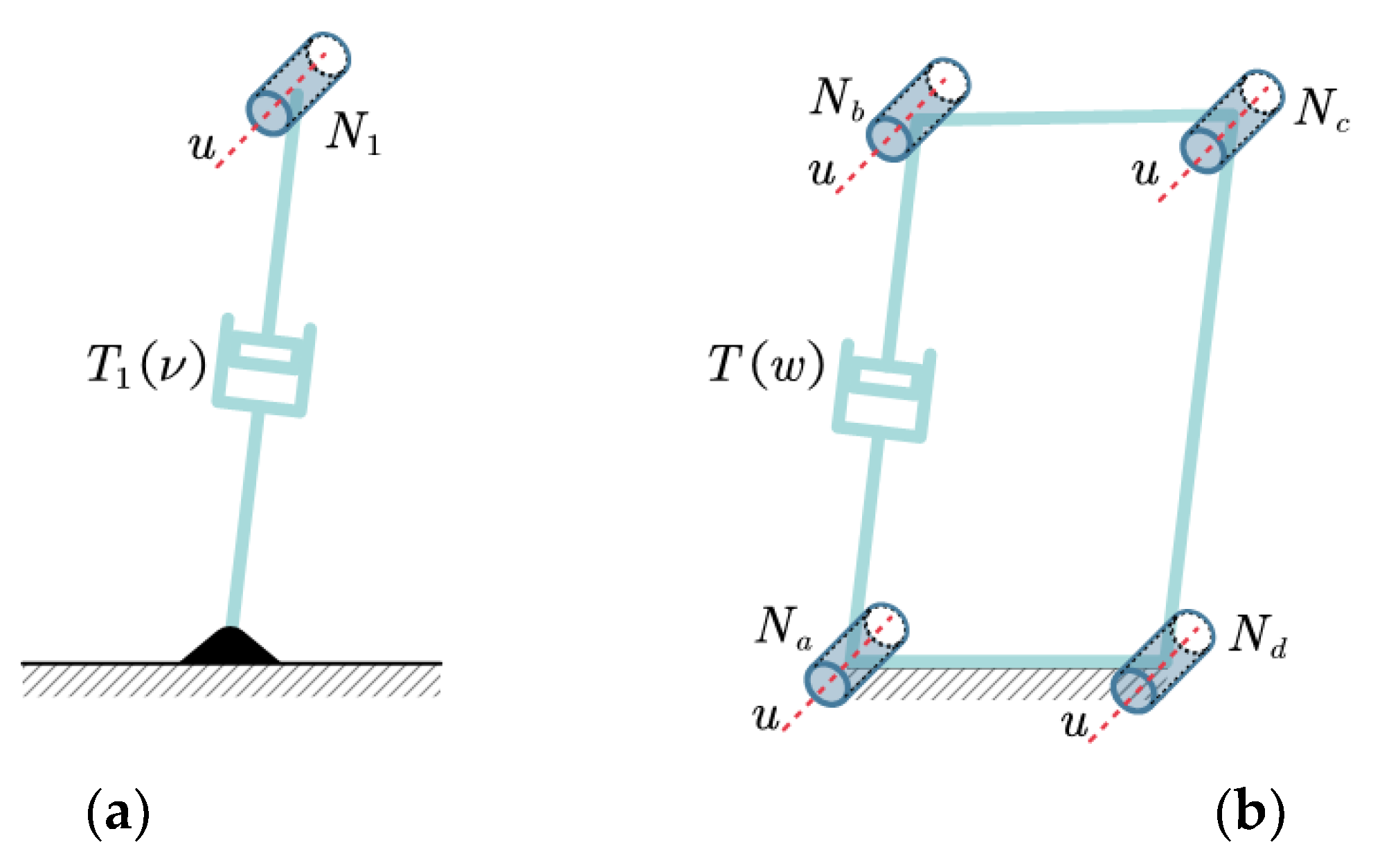
Figure 2.
A 2T1R-type parallel mechanism (a) three-dimensional physical model. (b) Simplified diagram of the mechanism.
Figure 2.
A 2T1R-type parallel mechanism (a) three-dimensional physical model. (b) Simplified diagram of the mechanism.
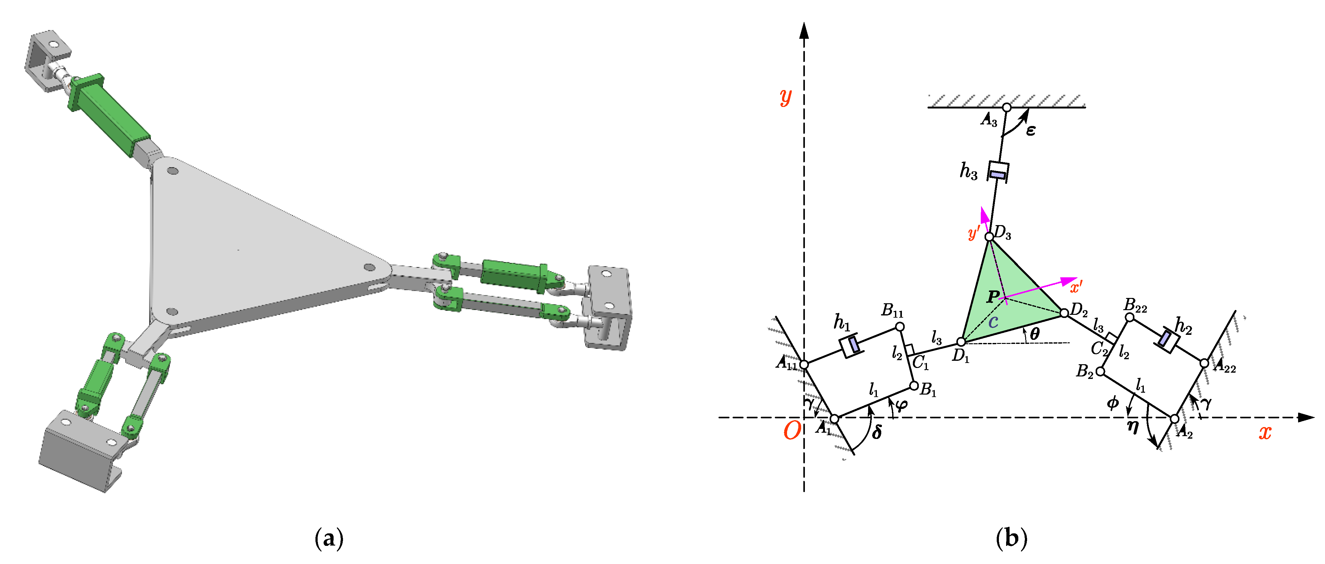
Figure 3.
Simulation model of the mechanism in ADAMS.

Figure 4.
Comparisons of inverse kinematics theory and simulation results: (a) ; (b) ; (c) .

Figure 5.
Comparisons of input velocity curves theory and simulation results: (a) ; (b) ; (c) .
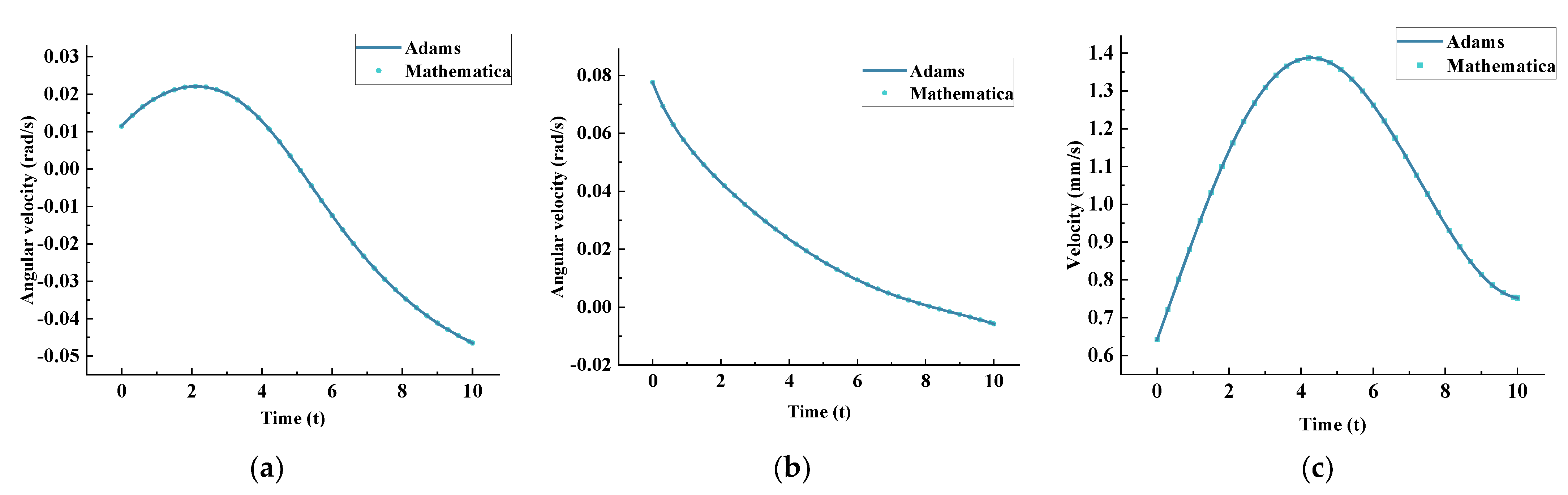
Figure 6.
End-effector workspace.
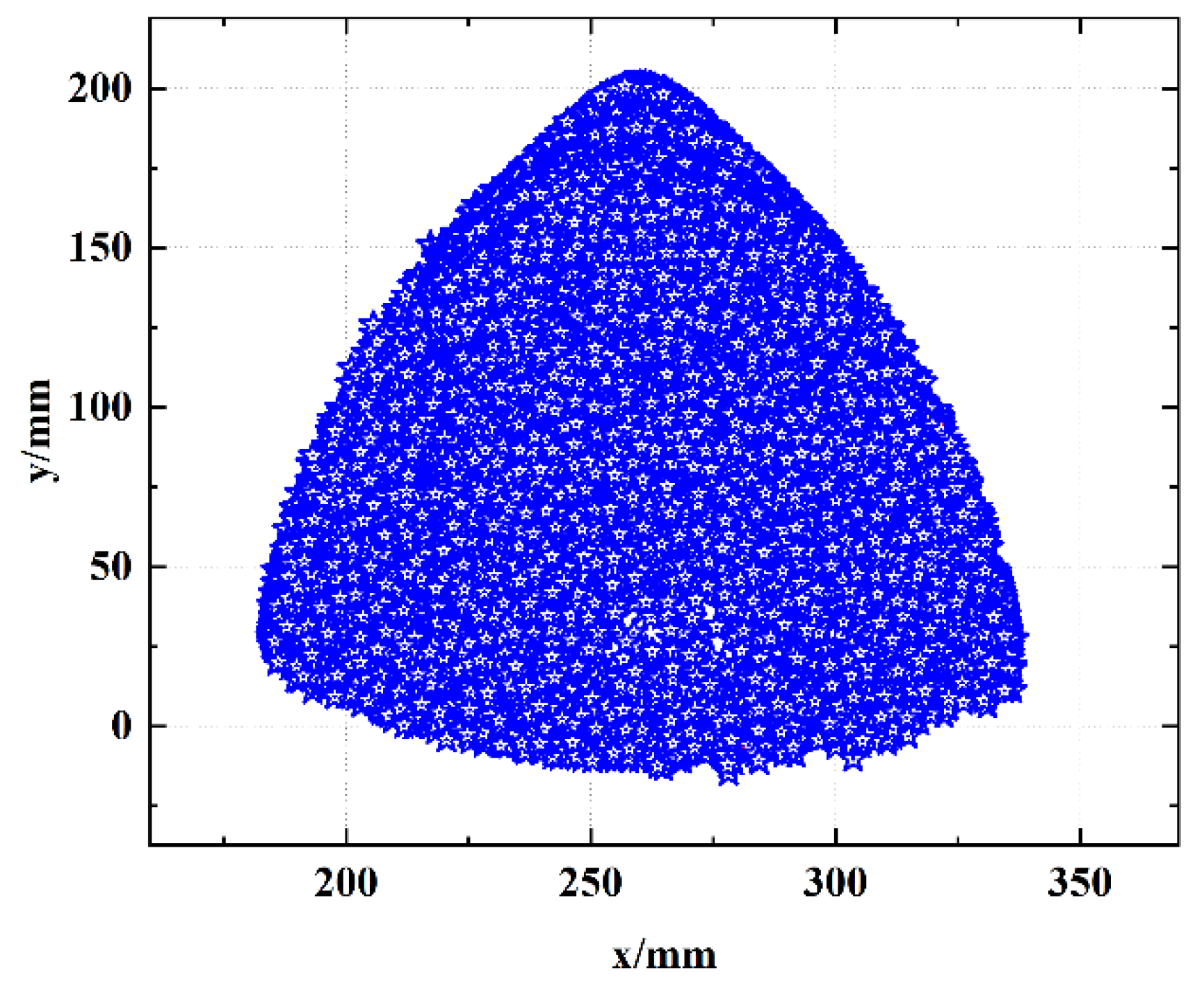
Figure 7.
Distribution diagram of stiffness index.
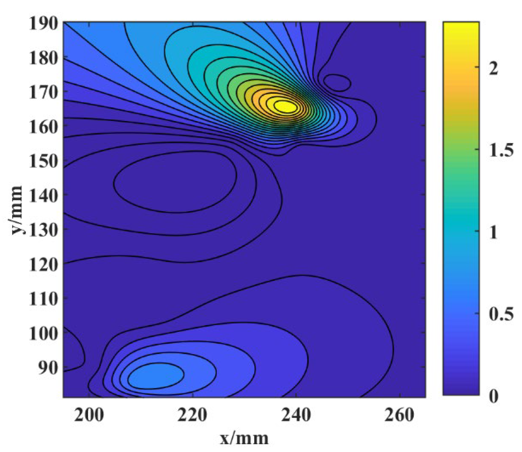
Figure 8.
Distribution diagram of dexterity index.
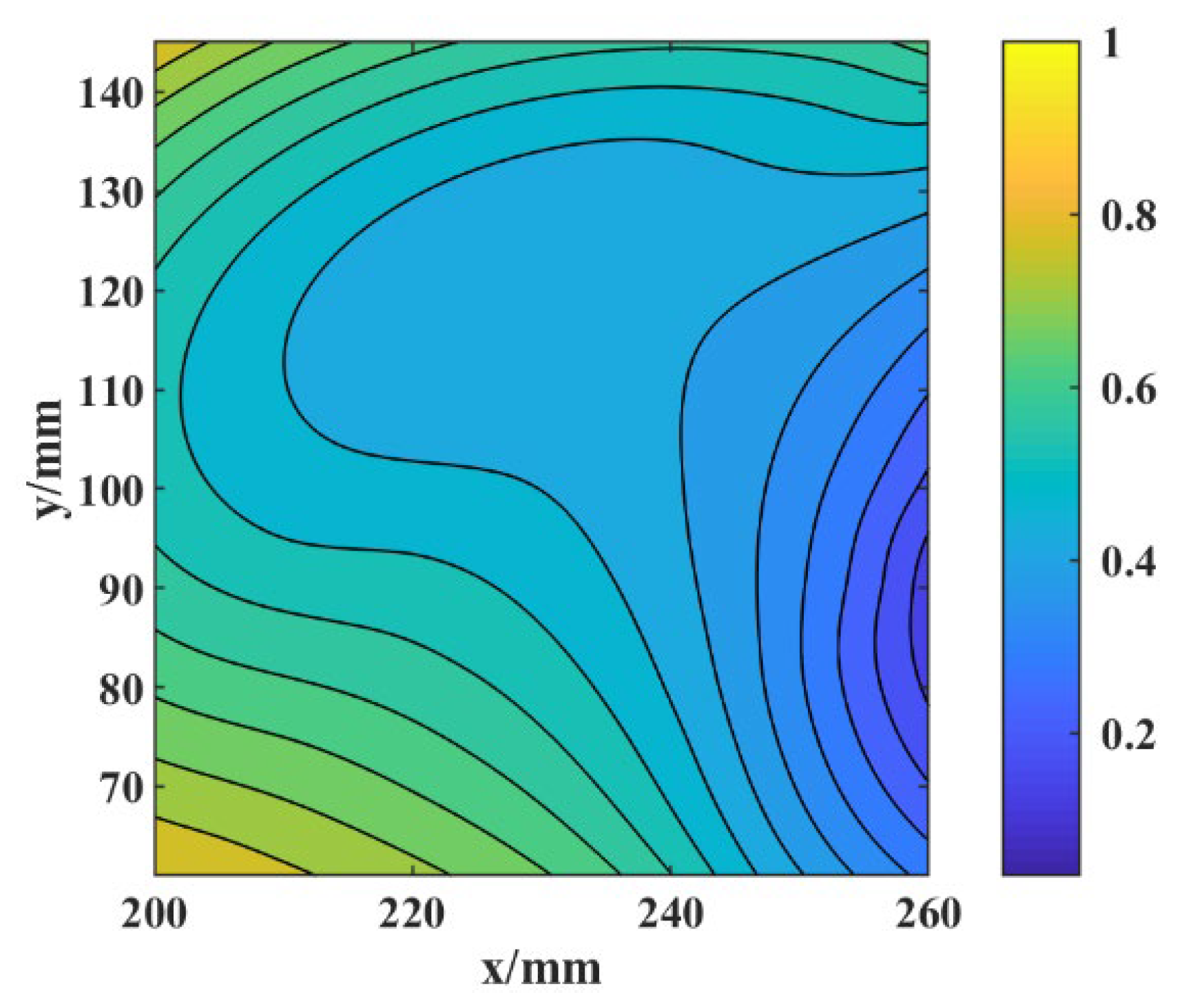
Figure 9.
Convergence graph of best fitness value.


Table 1.
The result of the type synthesis.
| Configuration | Constraint Space | DoF Space | Kinematic Chain |
|---|---|---|---|
| First limb | 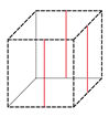 One-dimensional force constraint and two-dimensional couple constraint |  Two-dimensional translations and one-dimensional rotation |  (RR-RPR)-R |
| Second limb | 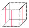 One-dimensional force constraint and two-dimensional couple constraint | 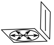 Two-dimensional translations and one-dimensional rotation |  (RR-RPR)-R |
| Third limb | 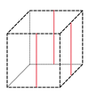 One-dimensional force constraint and two-dimensional couple constraint | 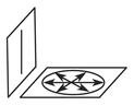 Two-dimensional translations and one-dimensional rotation |  RPR |
| Mechanism | 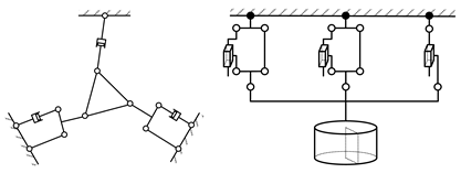 Two translational DoFs and one rotational DoF (  , ,  : Prismatic pair; : Prismatic pair;  : Revolute pair; : Revolute pair;  : Fixed point) : Fixed point) | ||
Table 2.
The parameters of the mechanism.
| Parameter | Value (mm) | Parameter | Value (mm) |
|---|---|---|---|
| 20 | 450 | ||
| 134 | 100 | ||
| 500 | 40 | ||
| 260 | 80 | ||
| h1 | (45, 135) | h2 | (45, 135) |
Table 3.
The workspace parameters of the mechanism.
| Parameter | Minimum Value | Maximum Value |
|---|---|---|
| X | 177.75 mm | 341.22 mm |
| Y | −6.51 mm | 201.37 mm |
| 0° | 90° | |
| 0° | 97° | |
| 0° | 94° | |
| 115 mm | 331 mm |
Table 4.
Variable constraints.
| Variable | Constrants (mm) | Variable | Constrants (mm) |
|---|---|---|---|
| l1 | 70,150 | l3 | 50,100 |
| l2 | 3070 | c | 60,110 |
Table 5.
Optimized design variables.
| Number | l1 | l2 | l3 | c | Number | l1 | l2 | l3 | c |
|---|---|---|---|---|---|---|---|---|---|
| 1 | 122.33 | 60.43 | 76.46 | 105.51 | 16 | 148.16 | 53.72 | 83.50 | 106.35 |
| 2 | 149.55 | 30.77 | 87.86 | 76.30 | 17 | 134.42 | 69.74 | 65.97 | 100.10 |
| 3 | 110.40 | 43.34 | 94.95 | 88.59 | 18 | 149.79 | 62.94 | 78.92 | 64.27 |
| 4 | 115.93 | 40.61 | 99.92 | 101.53 | 19 | 125.14 | 34.19 | 69.15 | 86.13 |
| 5 | 145.04 | 53.29 | 52.16 | 108.27 | 20 | 114.68 | 54.79 | 69.02 | 103.86 |
| 6 | 117.85 | 52.73 | 75.35 | 86.10 | 21 | 127.92 | 58.95 | 53.49 | 98.18 |
| 7 | 134.38 | 35.75 | 86.65 | 83.83 | 22 | 116.65 | 60.65 | 90.99 | 106.06 |
| 8 | 107.08 | 58.06 | 80.04 | 95.25 | 23 | 144.73 | 67.56 | 58.16 | 103.34 |
| 9 | 130.24 | 34.02 | 64.50 | 98.35 | 24 | 107.88 | 67.58 | 68.37 | 103.65 |
| 10 | 121.66 | 56.24 | 89.78 | 91.65 | 25 | 121.83 | 60.72 | 53.53 | 102.34 |
| 11 | 137.60 | 45.83 | 62.47 | 83.27 | 26 | 145.47 | 43.75 | 93.90 | 90.22 |
| 12 | 122.47 | 52.57 | 66.86 | 93.96 | 27 | 85.55 | 63.56 | 67.35 | 97.22 |
| 13 | 117.70 | 51.60 | 75.05 | 87.02 | 28 | 101.36 | 51.12 | 90.21 | 107.50 |
| 14 | 130.94 | 38.76 | 90.12 | 74.80 | 29 | 106.34 | 60.34 | 83.12 | 105.12 |
| 15 | 144.78 | 68.38 | 71.68 | 78.30 | 30 | 129.38 | 31.82 | 51.48 | 104.85 |
Table 6.
Objective function values.
| No. | Value | No. | Value | No. | Value | No. | Value | No. | Value |
|---|---|---|---|---|---|---|---|---|---|
| 1 | 5.04 | 7 | 4.01 | 13 | 5.08 | 19 | 4.84 | 25 | 4.11 |
| 2 | 5.66 | 8 | 5.13 | 14 | 4.35 | 20 | 6.24 | 26 | 3.64 |
| 3 | 5.54 | 9 | 5.32 | 15 | 6.34 | 21 | 4.12 | 27 | 5.02 |
| 4 | 4.82 | 10 | 4.62 | 16 | 3.20 | 22 | 3.30 | 28 | 4.64 |
| 5 | 4.80 | 11 | 4.21 | 17 | 5.35 | 23 | 4.79 | 29 | 4.14 |
| 6 | 6.70 | 12 | 5.02 | 18 | 6.03 | 24 | 4.85 | 30 | 5.72 |
Publisher’s Note: MDPI stays neutral with regard to jurisdictional claims in published maps and institutional affiliations. |
© 2022 by the authors. Licensee MDPI, Basel, Switzerland. This article is an open access article distributed under the terms and conditions of the Creative Commons Attribution (CC BY) license (https://creativecommons.org/licenses/by/4.0/).
Share and Cite
MDPI and ACS Style
Wang, D.; Zhang, J.; Guo, H.; Liu, R.; Kou, Z. Design of a 2T1R-Type Parallel Mechanism: Performance Analysis and Size Optimization. Actuators 2022, 11, 262. https://doi.org/10.3390/act11090262
AMA Style
Wang D, Zhang J, Guo H, Liu R, Kou Z. Design of a 2T1R-Type Parallel Mechanism: Performance Analysis and Size Optimization. Actuators. 2022; 11(9):262. https://doi.org/10.3390/act11090262
Chicago/Turabian StyleWang, Dongbao, Jing Zhang, Hongwei Guo, Rongqiang Liu, and Ziming Kou. 2022. "Design of a 2T1R-Type Parallel Mechanism: Performance Analysis and Size Optimization" Actuators 11, no. 9: 262. https://doi.org/10.3390/act11090262
Note that from the first issue of 2016, this journal uses article numbers instead of page numbers. See further details here.