Impact of Service Life on the Environmental Performance of Buildings

Abstract

The environmental performance assessment of the building and construction sector has been in discussion due to the increasing demand of facilities and its impact on the environment. The life cycle studies carried out over the last decade have mostly used an approximate life span of a building without considering the building component replacement requirements and their service life. This limitation results in unreliable outcomes and a huge volume of materials going to landfill. This study was performed to develop a relationship between the service life of a building and building components, and their impact on environmental performance. Twelve building combinations were modelled by considering two types of roof frames, two types of wall and three types of footings. A reference building of a 50-year service life was used in comparisons. Firstly, the service life of the building and building components and the replacement intervals of building components during active service life were estimated. The environmental life cycle assessment (ELCA) was carried out for all the buildings and results are presented on a yearly basis in order to study the impact of service life. The region-specific impact categories of cumulative energy demand, greenhouse gas emissions, water consumption and land use are used to assess the environmental performance of buildings. The analysis shows that the environmental performance of buildings is affected by the service life of a building and the replacement intervals of building components.

1. Introduction

A building is a complex product of different components of variable materials, structural importance, functional life, exposure constraints, and damage mechanisms. Each component of a building has a typical functional requirement and it should perform as per the prescribed function in its service life. Life cycle assessment (LCA) studies that have been conducted, to date, consider the service life of building and building components between 30 and 70 years with a most commonly used value of 50 years (

Table 1. Existing case studies.

Author	Life Span (Years)	Impact Indicators
Ramesh et al. [8]	75	Life cycle energy demand
Allacker K. [9]	60	External costs
Audenaert A. [10]	50	Waste generation
Carre A. [11]	60	Global warming potential (GWP), Cumulative energy demand (CED), water use, solid waste, photochemical oxidation, eutrophication, land use, and resource depletion
Iyer-Raniga U. [12]	100	Carbon emission, energy, photochemical oxidation, eutrophication, land use and water use
Rouwette R. [13]	50	GHG, CED
Cuellar-Franca R.M. [14]	50	GWP, acidification, eutrophication, abiotic depletion, ozone depletion, photochemical ozone creation, human toxicity
Nemry F. [15]	40	GWP, primary energy, acidification, eutrophication, ozone depletion, photochemical, ozone creation
Ortiz O. [16]	50	GWP, acidification, human toxicity, abiotic depletion, ozone depletion
Crawford et al. [6]	50	Embodied energy, cost, operational energy
Cabeza et al. [17]	30 to 100 mostly 50	Life cycle energy
Biswas W.K. [18]	50	GHG emissions, Embodied energy (EE)
Islam H. [19]	50	Life cycle energy, life cycle cost (LCC)
Atmaca A. [20]	30 to 100 mostly 50	GHG emissions
Lawania K.K. [21]	50	GHG emissions, life cycle energy
Grant A. [1]	Estimated	GWP, atmospheric ecotoxicity, atmospheric acidification
Dixit M.K. [22]	50	Embodied energy
Vitale P. [23]	50	GWP, respiratory inorganics potential, non-renewable energy potential, waste framework directive
Vitale P. [24]	50	Respiratory inorganics, GWP, non-renewable energy
Balasbaneh A.T. [25]	50	GWP, human toxicity, acidification, eutrophication, LCC, labor wage rate, job creation

). However, the real picture is quite contradictory to these assumptions as the service life of buildings varies with materials, operation and maintenance and the surrounding environment [1,2]. This discrepancy may lead to inaccuracy of LCA analyses, and material and energy balance. Any building needs regular maintenance and replacement of its non-structural components to keep the building in performing conditions. In second half of the 20th century, a considerable number of buildings were constructed that need annual inspections and maintenance, influencing the national economy and competitive position of the construction industry [3]. The maintenance and replacement intervals of existing buildings need to be optimized to achieve environmental, social and economic benefits. For new constructions, the estimated intervals of maintenance and replacements should be planned as concisely and wisely as possible. The integration of knowledge of building component durability and its structural and functional performance into building LCA could help conduct a realistic assessment of the environmental performance of building components [4]. Due to the uncertainty associated with the use of assumed service life of a building, as well as the unavailability of service life data of building components, LCA studies have not frequently addressed the real energy consumed during maintenance and replacement activities. However, this energy (hereafter, named replacement energy) may be as much as 7% to 110% of the initial embodied energy, if the service life of building materials is not properly implemented in the design phase of a building [4,5,6,7]. The building life span, whether short or long, has discretionary effects on a building’s environmental performance. Short service life of buildings results in excessive solid waste, embodied energy and subsequent greenhouse gas (GHG) emissions during pre-use stage (extraction of material to construction). Long service life of buildings increases replacement of building components, resulting in an increase of replacement energy and prolonged use stage, increasing operational energy and GHG emissions [1]. These two constraints need to be taken into account during material selection by considering the service life of the whole building, as well as its components, and is essential to achieve environmental performance while fulfilling social and economic objectives.

According to ISO 15686-1, “Service life is the period of time after construction, in which a building and its parts meet or exceed the acceptable minimum requirements of performance established” [26]. The service life of building components largely depends on the materials’ properties, damage mechanisms, environment and quality of design, and work execution. This study aims to estimate the service life of buildings and building components and expected replacement intervals of non-structural components, and to assess the impact of this service life on life cycle environmental performance of buildings.

1.1. Service Life Estimation

Service life (SL) estimation of buildings is quite a complicated process that involves intensive data analysis as there is no proto-type in buildings. Each building is unique in its composition, material specification and architectural and structural design. Therefore, the SL estimation cannot be generalized and needs to be carried out on a component to component basis. Construction materials have different properties and damage mechanisms and behave differently in different climates. User requirements, degradation agents, and building performance against these agents are important factors to consider for service life planning [27]. The state-of-the-art report on performance-based methods on service life prediction states that “Prediction of durability is subject to many variables and cannot be an exact science” [28]. Therefore, efforts should be made to achieve the most likely estimate by considering the most reliable data sources.

SL prediction methods should be generalized, easy to apply to a variety of materials, user friendly and give clear boundary limitations [29]. SL was first studied by Legget and Hutcheon in 1958. However, SL estimation has been under the limelight since the 1990s by different standard institutes. The Guidelines for Service Life Planning were first published by the Architectural Institute of Japan (AIJ) in 1989 followed by British Standard Institute (BSI) in 1992 and Canadian Standards Association (CSA) in 1995. International standard organizations (ISO) published ISO 15686-1, Building and constructed assets—Service Life Planning—Part 1 in 2000 [30]. A series of publications on ISO 15686 were published afterwards, covering different aspects and procedures of service life predictions.

Service life can be estimated by deterministic, engineering and probabilistic methods. The probabilistic method is the research approach considering degradation probability of a building during a prescribed time. The deterministic method is a simple approach utilizing factors influencing the degradation of a building under certain conditions. The factor method, described in standard, ISO 15686-2 [31], is the well-known deterministic approach. Engineering methods lie somewhere in between deterministic and probabilistic methods. Engineering methods are easy, and use the time-based degradation mechanism for interpretation [32]. SL estimation needs a wide range of data from different sources and under different conditions. These information resources may be existing building data, information collected by surveys, manufacturer data, service life modelling, insurance companies and real estate data, and expert opinion [33]. The engineering approach depends on structural properties of materials, loading conditions, chemical composition, and damage mechanisms in a buildings’ life time. However, there is a huge variety of chemical compositions in materials, degradation in different environments, and variable human influences, to treat all materials just the same. Accelerated life tests carried out on building components to predict SL give reasonably accurate results. It is still a big challenge to depict the realistic conditions for life tests. In addition, the accelerated tests are quite expensive. There are also some other approaches to predict SL by considering service life models and obsolescence factors [1,34]. This method can be used for existing buildings or to be built buildings with the same material. This method requires empirical data that cannot be collected for innovative materials. Acquiring data for service life models and time constraint can pose a challenge for the SL prediction approach.

The factor method is the deterministic method that uses seven factors to predict the service life behavior of the building in different climatic conditions and geographic locations. The factor method uses reference service life (RSL) of a building component as a baseline and seven factors to modify the RSL to estimated service life (ESL). The service life estimation is different from service life prediction in the sense that the first is meant for particular conditions, and the second is recorded performance over a prescribed time or referenced SL [30,35]. The factor method helps to estimate service life of building and building components using Equation (1) [30].

ESL = RSL × A × B × C × D × E × F × G,

(1)

where,

• ESL = Estimated service life of building components
• RSL = Reference service life of building components
• Factor A = Quality of components including manufacturing, storage, transport and protective coating etc.
• Factor B = Design level including incorporation, sheltering by rest of structure and surrounding buildings
• Factor C = Work execution level, site management, workmanship level, weather condition during work
• Factor D = Indoor environment conditions, humidity, ventilation, and condensation etc.
• Factor E = Outdoor environment, microenvironmental conditions, weathering factors, building elevation etc.
• Factor F = In-use conditions, mechanical impact, wear and tear, category user etc.
• Factor G = Maintenance level, quality and frequency.

The method incorporates the material behavior, human involvement and degradation mechanism to interpret the ESL. The factor method is flexible, and it considers the combined effect of different deteriorating factors. The method needs judgement of factors as protective or deteriorating and requires fair and definite limitations on factors to avoid complexity [36]. Reliable data is required for the RSL and factors for each building component. The availability of data and reliability of data sources play an important role in SL estimation. The data sources may be manufacturers of building products, test laboratories, government agencies reports, existing studies etc., [37]. The most challenging issue in SL estimation is how to use effectively the available data to predict the SL of a structure that is to be built. In this study, the service life was estimated for most likely values (±5 years) using the factor method.

1.2. Environmental Life Cycle Assessment

The environmental life cycle assessment (ELCA), frequently known as life cycle assessment is a comprehensive tool to assess the environmental impacts of a product or system or service, in pre-use, use, and post-use stages [38]. The ELCA was studied for the first time in the 1960s and up until the 1970s, it was used only to compare the packaging options of consumer goods. In 1969, the Midwest Research Institute conducted a study on LCA for a Coca Cola Company for different types of beverage containers [39]. The studies in this period revolved around policy making and enterprises with a focus on solid wastes, energy consumption, and air pollutant impacts. In the 1990s, SETAC, conducted various workshops and published the first code of practice for life cycle assessment in 1993 [40]. Afterwards, the international standards organization (ISO), was involved actively and published generalized procedures and methods for LCA in ISO 14040-44 in 1997–2000 [38].

In the construction sector, ELCA was first applied in 1980s by Bekker to study the environmental implications of the use of renewable resources in buildings [41]. ELCA was used in buildings to assess the environmental impacts of construction materials and is a credible solution to compare material sustainability [42,43,44,45]. Now, the ELCA covers a wide range of areas from building materials (i.e., bricks, cement etc.) to urban planning [46]. The life cycle stages that are usually considered from life cycle assessment of buildings and building components include pre-construction, construction, use and end of life stages. Environmental product declarations (EPDs) involved the use of LCA to estimate environmental impacts for environmental declaration purposes for certification purposes [47]. ELCA helps to improve the performance of building in its entire life span by first identifying hotspots and then by applying mitigation strategies [47,48]. However, the system boundaries, functional units and scope definition are unique for each building LCA study, resulting in variation in results among studies [49,50,51].

Environmental performance of buildings is also defined as a quantified relationship between occupant’s comfort level and environmental impacts [52,53,54]. Embodied and operational impacts are usually two main categories of environmental impacts. Embodied impacts are static and further divided into pre-use embodied impacts and replacement embodied impacts [6]. Pre-use embodied impacts are the impacts due to extraction, manufacturing and construction of buildings and replacement embodied impacts are a result of renovations, replacements and maintenance in the active service life of buildings. The operational or use stage impacts are dynamic in nature and occur in the service life of building [55,56]. Better building performance can be achieved by considering factors including material selection, construction techniques, cost factors, and cleaner production strategies (CPS).

Whilst Australia accounts for only 0.32% of the world’s population, its per capita GHG emission is extremely high compared to countries with similar economies (UK, Mexico, South Korea) i.e., 26 tonnes GHG emissions per capita per year as opposed to 13 tonnes per capita GHG emissions for South Korea, 10 tonnes per capita GHG emissions for UK and 20.3 tonnes per capita GHG emissions for Canada [57]. Australia is the second driest continent after Antarctica [58]. The annual rainfall is highly variable and central Australia is mostly arid with only 6% arable land in coastal areas [59]. Water is the most precious commodity and its scarcity is covered by desalination of sea water [60,61,62]. Water mapping in the construction industry helped to identify need for reducing the life cycle water demand/footprint of buildings by using renewable resources. In addition, Australia’s per capita waste generation is 2.6 tonnes per year as compared to 0.706 tonne per capita per year for US, out of which 0.8 tonnes per capita per year is construction and demolition waste [63]. Therefore, these two issues are inevitable for assessment of the environmental impacts of building and construction industry at the planning stage of buildings using an ELCA to discern strategies to avoid these environmental consequences. This study thus considered these impact categories, including cumulative energy demand, GHG emissions, water consumption and land use to assess the environmental performance of buildings.

2. Method

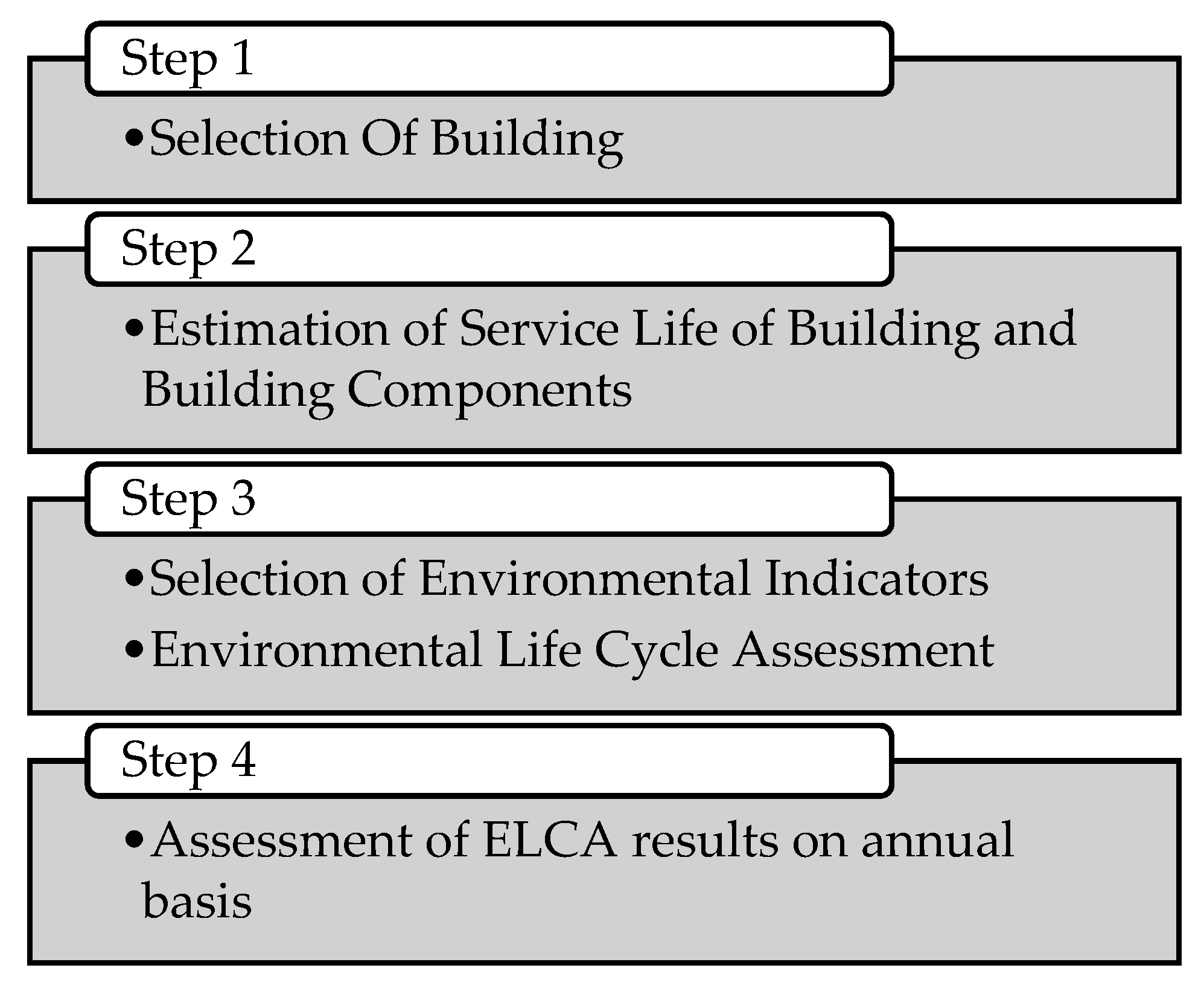
This study focuses on the impact of service life on environmental performance of buildings. The methodology consists of four main steps (Figure 1). Step 1: Twelve residential buildings were selected. All specifications of the buildings including the architectural design, covered area, orientation, and utility were the same except for the difference in building materials. The residential buildings were modelled using three main systems of roof, wall and footing.

The roof system comprised of roof cladding, roof frame, and suspended ceiling. The wall system comprised of exterior render, wall frame and interior plaster and the footing system comprised of footing slab and flooring. The variation in buildings was created only in materials of structural components. The materials for non-structural components were unchanged as replacements for these components are considered easy and does not affect the service life of the whole building. Two types of roof frames, two wall frames and three types of slab footings, resulted in 12 combinations of buildings (

Table 2. Building components of building combinations and the reference building.

Building	Building Specifications	Building Components
		Roof Frames	Wall Frames	Slab Footing
Building-50	TF-DB-CC	Timber frame	Double Brick	Conventional concrete
1	TF-CB-CC	Timber frame	Concrete Block	Conventional concrete
2	TF-CB-FAGC	Timber frame	Concrete Block	30% FA Green concrete
3	TF-CB-GGBFS	Timber frame	Concrete Block	30% GGBFS Green concrete
4	TF-DB-CC	Timber frame	Double Brick	Conventional concrete
5	TF-DB-FAGC	Timber frame	Double Brick	30% FA Green concrete
6	TF-DB-GGBFS	Timber frame	Double Brick	30% GGBFS Green concrete
7	SF-CB-CC	Steel Frame	Concrete Block	Conventional concrete
8	SF-CB-FAGC	Steel Frame	Concrete Block	30% FA Green concrete
9	SF-CB-GGBFS	Steel Frame	Concrete Block	30% GGBFS Green concrete
10	SF-DB-CC	Steel Frame	Double Brick	Conventional concrete
11	SF-DB-FAGC	Steel Frame	Double Brick	30% FA Green concrete
12	SF-DB-GGBFS	Steel Frame	Double Brick	30% GGBFS Green concrete

) and a conventional building named Building-50 composed of a timber roof frame, double brick walls and conventional concrete was considered as a reference case for comparison with the aforementioned 12 buildings.

Step 2: The service life of each building component was estimated using the factor method [37]. The service life of a system was taken as the service life of structural components i.e., ESL of the roof system was the value of service life for the roof frame. The least value of service life among building systems i.e., roof system, wall system and footing system, was taken as the estimated service life of the building [3]. The service life estimation of components was required, not only to determine the service life of the whole building, but also, to find the replacement intervals of non-structural components during the service life of a building. The service life of a reference building, Building-50 was assumed 50 years based on a literature review (Table 1).

Step 3: The indicators for environmental objective were selected by consulting existing studies. ELCA of the building was carried out as per ISO 14040-44 [38]. A quantitative life cycle inventory for building materials and transportation was compiled for construction, the subsequent replacements and demolishing activities. The ELCA considered a cradle to grave approach including pre-use (mining to material, transport of material to site and construction), use, post-use (demolition and disposal) and replacement (replacement of building components throughout the active service life of building) stages. ELCA software, SimaPro 8.4 [64], was used to determine the environmental indicators for impact categories of energy, GHG emissions, water consumption and land use.

Step 4: The impact values were presented on an annual basis for a service life of a building as estimated in the second step in order to investigate the impact of SL on environmental performance of buildings.

3. Case Studies

A typical house of four bedrooms and two bathrooms, with a covered area of 245.5 m² located in Perth WA, was selected for the case study. Twelve building combinations were created based on the roof, wall and footing systems, keeping architectural design, orientation, location and covered area constant (Table 2).

Each of the roof, wall and footing systems was modelled using structural and non-structural building components. Only the non-structural components were selected, that resulted in costly replacements and provided a thermal envelope to the building. However, this aspect of the building enveloping components will be assessed in future study. The roof system included two types of roof assemblies: TF—timber roof frame, terracotta tiles and gypsum board ceiling; and SF—steel roof frame, terracotta tiles and gypsum board ceiling. The wall system consisted of two types of wall assemblies: DB—double brick wall and interior plaster; and CB—concrete block wall, exterior render and interior plaster.

The footing system comprised of on-grade slab footing and ceramic tile flooring with three types of concrete mixes: CC—conventional concrete; 30% FA—Green concrete with 30% replacement of Ordinary Portland Cement (OPC) by class F fly ash; 30% GGBFS—Green concrete with 30% replacement of OPC by ground granulated blast furnace slag (GGBFS). The building systems were developed based on the most commonly used materials, in Western Australia with a design life of 50 years as proposed by National Building Codes. A conventional residential building with a timber roof, double brick walls and conventional concrete slab footing and 50-year service life was used as the reference building, Building-50.

A thorough study was conducted to collect the service life data of the building components used in the case study. Based on the gathered information, ranking criteria were set for each factor, to get most likely values (ESL ± 5 years) of ESL (

Table 3. Criteria and Coefficients of service life estimation

Factor Description		Roof System				Wall System				Footing System
Factor	Criteria	Timber Truss	Steel Truss	Terracotta Tiles	Gypsum board	Concrete Block	Double Brick	Plaster	Render	CC	30% FAGC	30% GGBFS	Ceramic Tiles
A	A = 1.1, Best Available Material; A = 1.05, Good Material; A=1.0, N/A-No effects; A = 0.95, Slightly low Standard material; A = 0.90, Low Standard Material	1.10	1.10	1.10	1.10	1.10	1.10	1.05	1.05	1.05	1.05	1.10	1.10
B	B = 1.1, Best Design with special considerations to strengthen the structure; B = 1.05, Good Design, (as per standards approach); B = 1.0, N/A-No effects; B = 0.95, low Standard design; B = 0.90, poor design	1.05	1.05	1.00	1.00	1.10	1.10	1.05	1.05	1.05	1.05	1.05	1.00
C	C=1.1, Satisfaction Level ≥ 90%; C = 1.05, 80% < Satisfaction Level > 90%; C = 1.0, N/A-No effect; C = 0.95, 70% < Satisfaction Level > 80%; C = 0.9, Satisfaction Level ≤ 70%	0.90	0.90	0.90	1.05	0.90	0.90	0.90	0.95	0.95	0.95	0.95	0.90
D	NOT CONSIDERED	1.00	1.00	1.00	1.00	1.00	1.00	1.00	1.00	1.00	1.00	1.00	1.00
E	E = 1.1, Supportive; E = 1.05, mild; E = 1.0, N/A-No effect; E = 0.95, Harsh; E = 0.9, Reactive	1.05	1.05	0.95	1.00	1.00	1.00	1.00	0.90	0.90	1.05	1.05	1.00
F	NOT CONSIDERED	1.00	1.00	1.00	1.00	1.00	1.00	1.00	1.00	1.00	1.00	1.00	1.00
G	G = 1.1, Best quality and interval as specified by manufacturer/designer; G = 1.05, good quality and interval as per requirement; G = 1.0, N/A-NO EFFECT; G = 0.95, low quality and as per required; G = 0.9, poor quality	1.05	1.05	1.05	1.05	1.00	1.00	1.05	1.05	1.00	1.00	1.00	1.05
RSL	Primary source [80% reliability] = manufacturers technical sheets, EPDs	50	75	50	25	60	75	25	15	60	60	60	50
ESL	Secondary source [60% reliability] = Databases like NAHB, BOMA; literature; experimental studies; codes and practices;	57	86	49	30	65	82	26	15	57	66	69	52

). Factor A, B, C, E, G were assigned ranking values from 1.1 to 0.9 [37], and Factor D, F were not considered in the study as these are dependent on occupant behavior and vary greatly. These factors were assigned a value of 1.0 in service life estimation equation. The factor values were reduced to increase the confidence level as compared to previously used values to test the sustainability framework for Building 1 and 2 [65].

The manufacturer data, life expectancy databases of building components and existing case studies were used as data sources for RSL. The manufacturer’s technical data sheets were consulted to set the component quality. The factor B values were assigned by considering commonly used practices in building design in Western Australia. Building commission WA annual reports were consulted to estimate the construction works execution level. The climatic conditions, reports of Bureau of Meteorology Western Australia, and inspection reports of residential buildings were considered for weighting outdoor climatic conditions and subsequent effect on the building components.

The life cycle assessment software SimaPro 8.4 was used to assess the environmental impacts of buildings with a grave to cradle approach. Materials required for each building were estimated for building construction and successive replacements. The transportation distances were calculated for nearest available materials retailers and manufacturers. The energy consumption during the use stage was estimated for thermal comfort, hot water, lighting and home appliances. AccuRate sustainability software [66] was used to estimate the annual cooling, heating, and hot water demand. The life cycle inventories for materials, energy consumption and transportation distances were compiled to incorporate in the SimaPro (

Table A1. Life cycle inventory of materials for the construction stage of case study buildings.

Material (tonnes)	Building-50	1. TF-CB-CC	2. TF-CB-FAGC	3. TF-CB-GGBFS	4. TF-DB-CC	5. TF-DB-FAGC	6. TF-DB-GGBFS	7. SF-CB-CC	8. SF-CB-FAGC	9. SF-CB-GGBFS	10. SF-DB-CC	11. SF-DB-FAGC	12. SF-DB-GGBFS
1. Excavation of foundation	26.83	26.83	26.83	26.83	26.83	26.83	26.83	26.83	26.83	26.83	26.83	26.83	26.83
2. Sand: Sub-base	26.01	26.01	26.01	26.01	26.01	26.01	26.01	26.01	26.01	26.01	26.01	26.01	26.01
3. On grade slab (including water proofing membrane, mesh reinforcement, ready mix concrete-N20)	79.56	79.56	79.56	79.56	79.56	79.56	79.56	79.56	79.56	79.56	79.56	79.56	79.56
4. Floor Tiles (Ceramic)	5.47	5.47	5.47	5.47	5.47	5.47	5.47	5.47	5.47	5.47	5.47	5.47	5.47
5. Concrete Blocks wall (including mortar, steel rebar, metal lintels)		75.78	75.78	75.78				75.78	75.78	75.78
6. Bricks (including mortar, metal lintels)	107.4				107.4	107.4	107.4				107.4	107.4	107.4
7. Plaster	10.54	10.54	10.54	10.54	10.54	10.54	10.54	10.54	10.54	10.54	10.54	10.54	10.54
8. Rendering		13.86	13.86	13.86				13.86	13.86	13.86
9. Gypsum board ceiling	2.19	2.19	2.19	2.19	2.19	2.19	2.19	2.19	2.19	2.19	2.19	2.19	2.19
10. Roof Timber (including bat insulation)	4.61	4.61	4.61	4.61	4.61	4.61	4.61
11. Roof Steel (including bat insulation)	x	x	x	x	x	x	x	2.33	2.33	2.33	2.33	2.33	2.33
12. Terracotta roof tiles	16.55	16.55	16.55	16.55	16.55	16.55	16.55	16.55	16.55	16.55	16.55	16.55	16.55
13. Metal door frames: 12 no.	0.18	0.18	0.18	0.18	0.18	0.18	0.18	0.18	0.18	0.18	0.18	0.18	0.18
Door shutters: 12 no.	0.37	0.37	0.37	0.37	0.37	0.37	0.37	0.37	0.37	0.37	0.37	0.37	0.37
14. Aluminum windows: Single glazed	1.43	1.43	1.43	1.43	1.43	1.43	1.43	1.43	1.43	1.43	1.43	1.43	1.43
Total material transported to construction site	254.3	236.5	236.5	236.5	254.3	254.3	254.3	234.3	234.3	234.3	252	252	252
Total material transported to landfill	26.83	26.83	26.83	26.83	26.83	26.83	26.83	26.83	26.83	26.83	26.83	26.83	26.83

,

Table A2. Life cycle inventory of materials for the replacement stage of case study buildings.

Material (tonnes)	Building-50	1. TF-CB-CC	2. TF-CB-FAGC	3. TF-CB-GGBFS	4. TF-DB-CC	5. TF-DB-FAGC	6. TF-DB-GGBFS	7. SF-CB-CC	8. SF-CB-FAGC	9. SF-CB-GGBFS	10. SF-DB-CC	11. SF-DB-FAGC	12. SF-DB-GGBFS
Terracotta tiles		16.55	16.55	16.55	16.55	16.55	16.55	16.55	16.55	16.55	16.55	16.55	16.55
Gypsum board		2.19	2.19	2.19	2.19	2.19	2.19	2.19	4.38	4.38	2.19	4.38	4.38
Plaster		21.08	21.08	21.08	21.08	21.08	21.08	21.08	21.08	21.08	21.08	21.08	21.08
Render		41.58	41.58	41.58	n/a	n/a	n/a	41.58	55.44	55.44	n/a	n/a	n/a
Ceramic tiles		0	0	0	0	0	0	0	5.47	5.47	0	5.47	5.47
Total material transported to site for replacement works		81.4	81.4	81.4	39.8	39.8	39.8	81.4	102.9	102.9	39.8	47.5	47.5
Total material transported to landfill		81.4	81.4	81.4	39.8	39.8	39.8	81.4	102.9	102.9	39.8	47.5	47.5

,

Table A3. Life cycle inventory of material transportation for the construction stage of case study buildings.

Carriage (tkm)	Building-50	1. TF-CB-CC	2. TF-CB-FAGC	3. TF-CB-GGBFS	4. TF-DB-CC	5. TF-DB-FAGC	6. TF-DB-GGBFS	7. SF-CB-CC	8. SF-CB-FAGC	9. SF-CB-GGBFS	10. SF-DB-CC	11. SF-DB-FAGC	12. SF-DB-GGBFS
Sand for levelling	1300.5	1300.5	1300.5	1300.5	1300.5	1300.5	1300.5	1300.5	1300.5	1300.5	1300.5	1300.5	1300.5
Material to site	6848.4	6316.2	6316.2	6316.2	6848.4	6848.4	6848.4	6247.8	6247.8	6247.8	6780	6780	6780
Construction waste	342.42	315.81	315.81	315.81	342.42	342.42	342.42	312.39	312.39	312.39	339	339	339
Dirt to landfill	1341.5	1341.5	1341.5	1341.5	1341.5	1341.5	1341.5	1341.5	1341.5	1341.5	1341.5	1341.5	1341.5
Material to landfill	1683.92	1657.31	1657.31	1657.31	1683.92	1683.92	1683.92	1653.89	1653.89	1653.89	1680.5	1680.5	1680.5

,

Table A4. Life cycle inventory of material transportation for the replacement stage of case study buildings.

Carriage (tkm)	Building-50	1. TF-CB-CC	2. TF-CB-FAGC	3. TF-CB-GGBFS	4. TF-DB-CC	5. TF-DB-FAGC	6. TF-DB-GGBFS	7. SF-CB-CC	8. SF-CB-FAGC	9. SF-CB-GGBFS	10. SF-DB-CC	11. SF-DB-FAGC	12. SF-DB-GGBFS
Material to site		2442.0	2442.0	2442.0	1194.6	1194.6	1194.6	2442.0	3087.6	3087.6	1194.6	1424.4	1424.4
Construction waste		122.1	122.1	122.1	59.7	59.7	59.7	122.1	154.4	154.4	59.7	71.2	71.2
Material to landfill		4070.0	1341.5	1341.5	1991.0	1991.0	1991.0	4070.0	5146.0	5146.0	1991.0	2374.0	2374.0
Total material to landfill		4192.1	1463.6	1463.6	2050.7	2050.7	2050.7	4192.1	5300.4	5300.4	2050.7	2445.2	2445.2

and

Table A5. Life cycle inventory of energy for the use stage of case study buildings.

Energy	Energy Consumption GJ/year
Non-thermal energy (home appliances, lighting)	18.834
Thermal energy (heating/cooling)	10.430
Natural gas consumption (hot water)	22.610
Total energy (use stage)	51.874

).

Table 4. Environmental Impact indicators

Impact Category	Impact Indicators	Impact Assessment Methods
Energy	Cumulative energy demand	Cumulative Energy Demand V1.09
GHG emissions	Life cycle GHG emissions	IPCC 2013 GWP 100a V1.02
Land use	Land use	Ecological footprints Australian V1.00
Water consumption	Resource depletion	Pfister et al. 2009 (Eco-indicator 99) V1.02

shows the environmental impact categories, impact indicators and methods used to assess the environmental impacts. These impact indicators were selected based on literature review and relevance to the scope of the study.

4. Results and Discussion

4.1. Estimated Service Life

The ESL of buildings and building components are presented in

Table 5. Estimated service life of building systems and buildings.

Service Life (Years)	TF-CB-CC	TF-CB-FAGC	TF-CB-GGBFS	TF-DB-CC	TF-DB-FAGC	TF-DB-GGBFS	SF-CB-CC	SF-CB-FAGC	SF-CB-GGBFS	SF-DB-CC	SF-DB-FAGC	SF-DB-GGBFS
	1.	2.	3.	4.	5.	6.	7.	8.	9.	10.	11.	12.
Roof System	57	57	57	57	57	57	86	86	86	86	86	86
Wall System	65	65	65	82	82	82	65	65	65	82	82	82
Footing System	57	66	69	57	66	69	57	66	69	57	66	69
Building	57	57	57	57	57	57	57	65	65	57	66	69

. The service life estimation shows that due to the large variation in service life of building components, enough life of building components is compromised. Approximately, 20% to 35% of ESL of structural components of 12 buildings, studied in this paper, is wasted. In buildings 4–7, the wall system has 82 years ESL that is 30.5% more than the ESL of the building. In buildings 10–12, the wall and roof systems both have higher ESL values than the footing system. In buildings 7–9, the roof system has a high ESL value compared to the wall and footing systems.

In building combinations 1–3, all the three systems have comparable ESLs that makes these the combinations with less material wastage at the post-use stage.

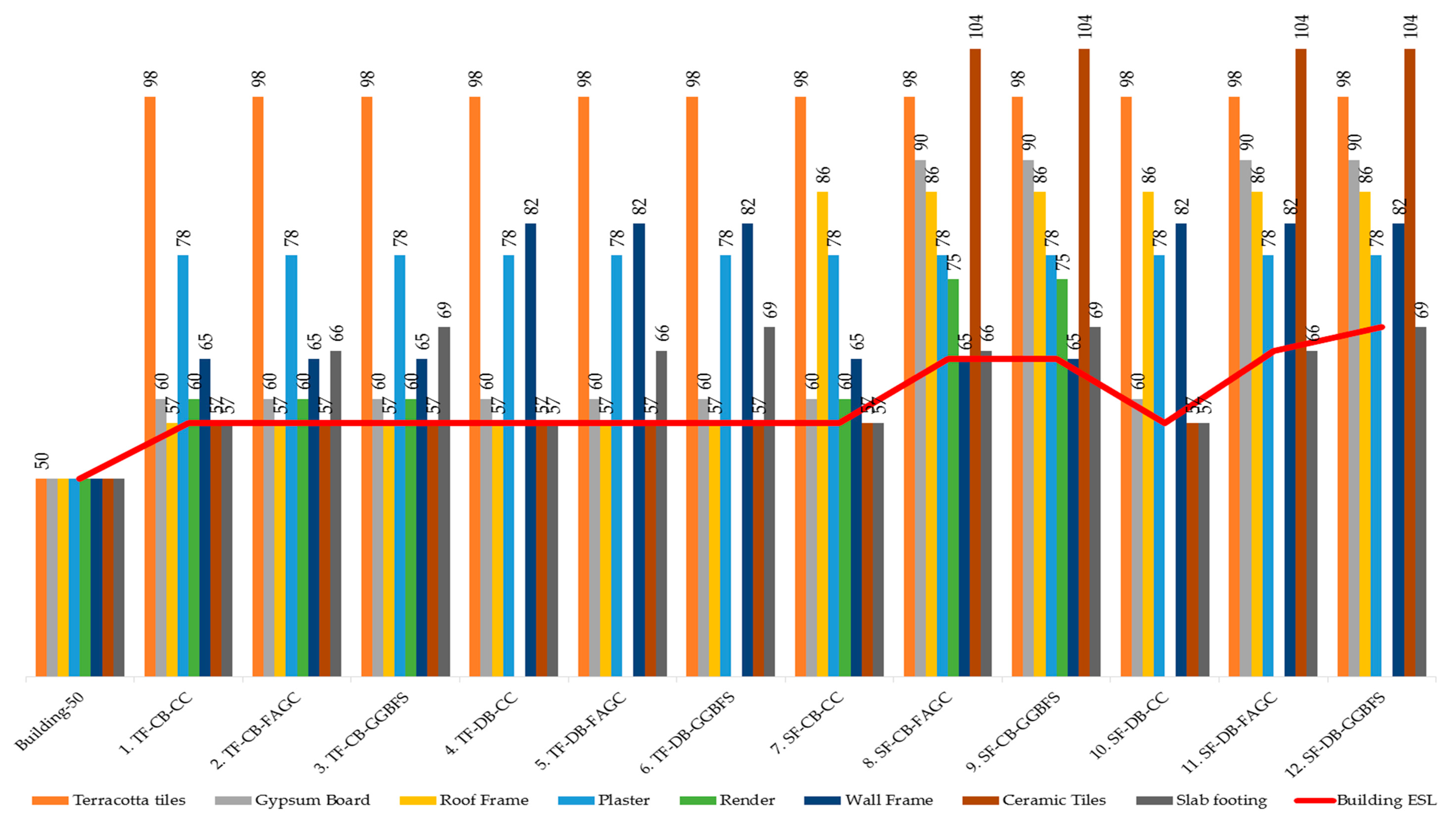
Based on the ESL of building components, the replacements of each building component in the ESL of buildings are specified. These ESLs are calculated conservatively considering that the components maintenance is carried out, strictly on schedule as described by the manufacturer or designer. No replacement is considered in the study for the building components within a range of ±5 years of the ESL of buildings [37]. This difference is assumed to be covered by maintenance. The ceramic floor tiles have an ESL of 52 years. As the ESL of ceramic tiles is within a range of ±5 years of the ESL of buildings 1–7 and 10, therefore, no replacement for ceramic tiles is suggested in the study. However, in buildings 8–9 and 11–12, one replacement of the ceramic floor tiles is considered. One replacement for terracotta tiles is considered for all buildings. The ESL of gypsum board ceiling needs to be replaced once in the ESL of buildings 1–7, 10 and twice in buildings 8–9, and 11–12. However, exterior rendering and interior plaster of walls need regular replacements after 15 and 26 years respectively, to maintain the aesthetic looks of buildings and to strengthen the concrete block wall against its inherent porous structure. Figure 2 shows the total ESL of building components at post-use stage including replacements. The red line shows the ESL of building and above this line is the remaining ESL of building components at the post-use stage. The remaining ESL is the duration for which a component is still in serviceable condition at the time of demolition of the building. The remaining life for structural components is the ESL of the component, however, the remaining life for non-structural components is calculated by multiplying the ESL of building components with number of replacements and subtracting from the ESL of building. The estimated number of replacements and remaining service life of building components is presented in

Table A6. Estimated number of replacements of building components in active service life of buildings.

Replacements of Building Components	Building-50	1. TF-CB-CC	2. TF-CB-FAGC	3. TF-CB-GGBFS	4. TF-DB-CC	5. TF-DB-FAGC	6. TF-DB-GGBFS	7. SF-CB-CC	8. SF-CB-FAGC	9. SF-CB-GGBFS	10. SF-DB-CC	11. SF-DB-FAGC	12. SF-DB-GGBFS
Building	50	57	57	57	57	57	57	57	65	65	57	66	69
Terracotta tiles	0	1	1	1	1	1	1	1	1	1	1	1	1
Gypsum board	0	1	1	1	1	1	1	1	2	2	1	2	2
Plaster	0	2	2	2	2	2	2	2	2	2	2	2	2
Render	0	3	3	3	n/a	n/a	n/a	3	4	4	n/a	n/a	n/a
Ceramic tiles	0	0	0	0	0	0	0	0	1	1	0	1	1

and

Table A7. Estimated Remaining life of building components at post-use stage of buildings.

Remaining Life (years)	Building-50	1. TF-CB-CC	2. TF-CB-FAGC	3. TF-CB-GGBFS	4. TF-DB-CC	5. TF-DB-FAGC	6. TF-DB-GGBFS	7. SF-CB-CC	8. SF-CB-FAGC	9. SF-CB-GGBFS	10. SF-DB-CC	11. SF-DB-FAGC	12. SF-DB-GGBFS
Building	50	57	57	57	57	57	57	57	65	65	57	66	69
Terracotta tiles		41	41	41	41	41	41	41	32	29	41	32	29
Gypsum board		3	3	3	3	3	3	3	25	25	3	24	21
Roof frame		0	0	0	0	0	0	29	21	21	29	20	17
Plaster		21	21	21	21	21	21	21	13	13	21	12	9
Render		3	3	3	n/a	n/a	n/a	3	10	10	n/a	n/a	n/a
Wall frame		8	8	8	25	25	25	8	0	0	25	16	13
Ceramic tiles		0	0	0	0	0	0	0	39	39	0	38	35
Slab footing		0	9	12	0	9	12	0	9	12	0	9	12

in Appendix A section. The study has shown that the lowest remaining life of building components at post-use stage (end of life of building), results in better environmental performance of building, due to reduced material wastage to landfill.

4.2. Cumulative Energy Demand

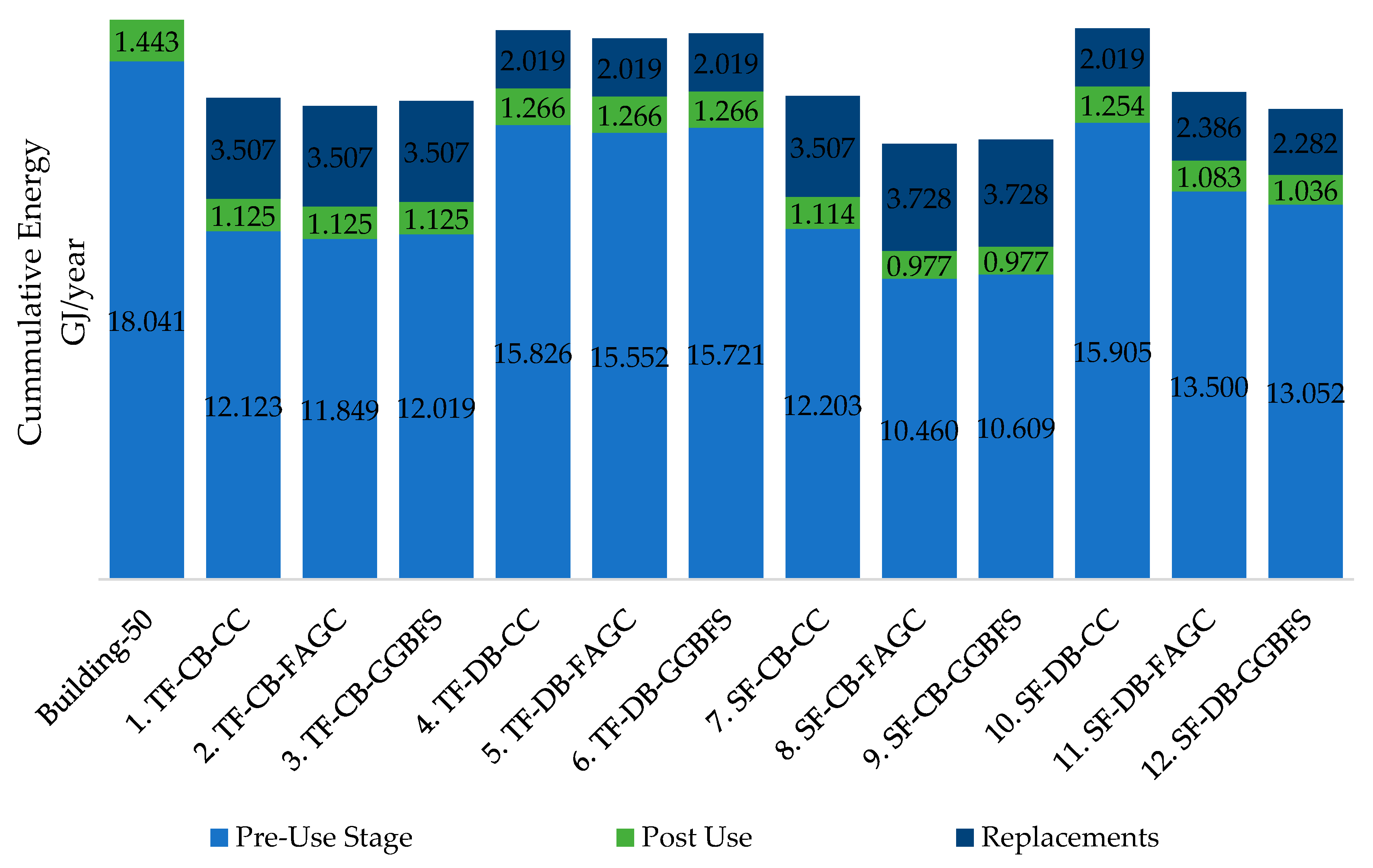
The cumulative energy demand (CED) is calculated on an annual basis to study the impact of service life on the environmental performance of buildings. The CED ranges from 97.799 to 101.813 GJ/year for 12 buildings. The CED is the highest in use stage with a value of 82.634 GJ/year and uniform in each case as no CPS is applied to buildings. The pre-use CED values are highest after the use stage due to energy consumed in extraction of raw materials, manufacturing of materials, transportation to site and construction activities. The replacement stage is the third main contributor to the CED of buildings (range from 2.02 to 3.73 GJ/year for 12 buildings), due to constant addition of embodied energy of replaced building components, at regular intervals (Table A6) during building service life. The post-use CED is negligible, as demolition and disposal of demolition waste to landfill ranges from 0.98 to 1.27 GJ/year for 12 buildings (1% of total energy demand) [4,67].

Figure 3 shows that CED is the lowest for building 8 (SF-CB-FAGC) with an ESL of 65 years i.e., 4.23% lower than the conventional Building-50 (TF-DB-CC) due to its longer ESL and the use of green concrete (OPC replaced by 30% FA). Similarly, the CED of building 9 (SF-CB-GGBFS) is 4.08% lower than Building-50, also mainly due to longer ESL. Buildings 4 (TF-DB-CC), 5 (TF-DB-FAGC), 6 (TF-DB-GGBFS) and building 10 (SF-DB-CC) have almost the same CED as Building-50 (102.118 GJ/year) with negligible differences between 0.37% and 0.63% owing to relatively shorter ESL than buildings 8–9, 11–12, and also because of the use of energy intensive structural material (e.g., double brick wall).

The longer ESL of building 12 (SF-DB-FAGC) and 11 (SF-DB-GGBFS) with ESL of 69 and 66 years, has reduced the share of pre-use energy consumption in comparison to buildings 4–6 and 10 that are composed of energy intensive brick walls and have an ESL of 57 years. Building 9 has the lowest energy demand in pre-use and post-use stage due to having low energy intensive concrete block wall and ESL of 65 years reducing per year share of CED of the building.

In the replacement stage, buildings with concrete block wall (1–3, 7–9) have high replacement embodied energy due to frequent replacements of energy intensive rendering and plastering. In buildings 8–9, the replacement embodied energies are highest due to ceramic tiles replacement in addition to rendering and plastering (Figure 2). Similarly, buildings 4–6, 10 with double brick walls have low replacement embodied energy as only interior plastering is replaced at a regular interval of 26 years (Table A6). Buildings 11 and 12, with longer ESL, have slightly higher replacement stage embodied energy due to replacement of ceramic tiles.

Although replacement embodied energy is higher in some buildings, the longer ESL of buildings reduces the impact of replacement embodied energy, as in buildings 8–9. In some cases, the use of energy intensive structural building components in fact reduced the overall CED of buildings. The steel frame roof is an energy intensive material, but its use had indirectly reduced the annual CED by increasing ESL of building combinations 8–9 and 11–12.

The results of this study were compared with similar studies in WA. Lawania and Biswas [68], estimated the annual CED for residential buildings across Western Australia showed slightly higher CED (138 GJ/year), which this value varies between 97.8 and 101.81 GJ/year under this current study. This variation happened due to the fact that Lawania and Biswas had used 18 different climatic locations and also one service life of 50 years was considered. In other studies of residential buildings that considered the embodied energy of building components replaced during ESL, embodied energy was found to increase by 20% to 40% due to increase of service life from 50 to 100 years [4,69,70]. Similar results were found for some buildings (buildings 8–9, 11–12) in the current study, where longer ESL had in fact increased the CED by 17% to 33% due to replacement of building components during ESL.

4.3. GHG Emissions

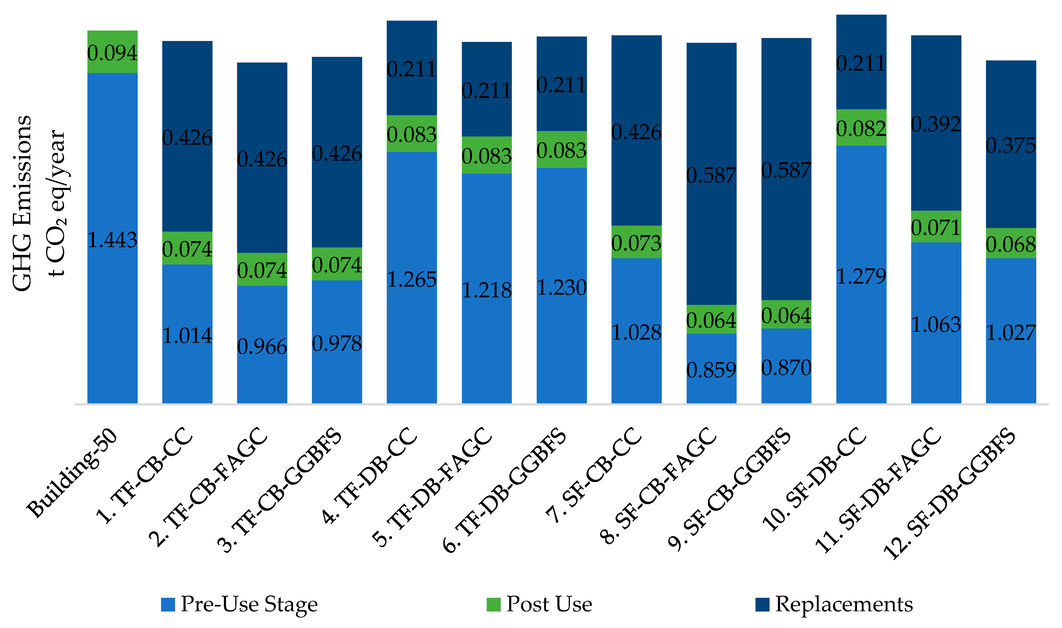
The GHG emissions in 12 buildings vary from 11.383 to 11.49 t CO₂ eq. The GHG emissions are highest in use stage with a value of 9.918 t CO₂ eq/year and uniform for all buildings like CED assessment due to use of electricity that is predominantly generated from fossil fuels (49% black coal and 36% gas) in WA [71]. The pre-use GHG emissions are highest after the use stage due to fossil fuel consumptions in extraction and manufacturing of materials, transportation of materials to site and construction equipment. The replacement stage is the third main contributor to the GHG emissions of buildings, due to the addition of the materials to building during ESL. The post-use CED is negligible as the demolition and disposal of demolition waste to landfill consumes only 1% of the total energy [4,67].

Building-50 (reference building) with a 50-year ESL, has annual GHG emissions of 11.455 t CO₂ eq/year, despite the absence of the replacement stage. Annual GHG emissions for building 2 (TF-CB-FAGC) with an ESL of 57-years, are the lowest among all the building combinations (i.e., 0.626% less than Building-50) due to use of low carbon intensive materials (timber, concrete blocks), less replacements of non-structural components (rendering, plastering) and most importantly due to having a similar ESL of building components as the whole building. These design specifications result in lower wastage of material or embodied energy at the post-use stage. Building 10 (SF-DB-CC) with an ESL of 57 years has the highest GHG emissions per year of 11.49 t CO₂ eq/year (i.e., 0.308% higher than Building 50) due to shorter ESL and use of energy intensive structural components (double brick wall, steel frame roof) with ESL longer than building ESL. It is worth mentioning that the building components with longer ESL than the whole building remains unused after the end of life demolition and disposal stage and are being considered as wastes.

Figure 4 shows that the double brick buildings 4 (TF-DB-CC), 5 (TF-DB-FAGC), 6 (TF-DB-GGBFS), and 10 (SF-DB-CC) have high pre-use stage annual GHG emissions of 1.265, 1.218, 1.230, and 1.279 t CO₂ eq/year, than Building-50, with 1.443 t CO₂ eq/year annual GHG emissions due to relatively longer ESL of 57 years and also due to use of energy intensive structural components i.e., brick walls (buildings 4–6, 10) and steel frame roof (building 10) with longer ESL (Figure 2) that is wasted to landfill at the post-use stage.

The GHG emissions associated with the replacement of components during the active service life are highest for building 8 (SF-CB-FAGC) and 9 (SF-CB-GGBFS) with a value of 0.587 t CO₂ eq/year. The reason for high replacement GHG emissions in these buildings is the use of carbon intensive ceramic tiles (13.07 t CO₂ eq) and rendering processes (10.56 t CO₂ eq). Additionally, the replaced ceramic tiles were not fully utilized as the ESL of buildings 8 and 9 expired at the 33% ESL of ceramic tile and therefore this valuable material was disposed along with other building materials into the landfill. The recovery of this carbon intensive material thus needs to be considered for use in similar applications during its remaining life (i.e., 67% of ESL). In addition, the rendering used large amounts of carbon intensive OPC (Ordinary Portland Cement). Nonetheless, due to the porous nature of concrete blocks, rendering or an alternative process is required to provide coverage to concrete blocks, which in fact increased the overall energy consumption as well as the GHG emissions.

Annual GHG emissions for case study buildings in the current study vary between 10.957 and 11.49 t CO₂ eq/year and is slightly higher than Lawania and Biswas [68,72] (9.4 t CO₂ eq/year). This is mainly due to differences in parameters like service life and climatic conditions affecting use stage GHG emissions. In a study by Carre A. [11] for Australian houses with a 50-year service life, pre-use GHG emissions (0.908 t CO₂ eq/year) are similar to current study (0.859 to 1.279 t CO₂ eq/year).

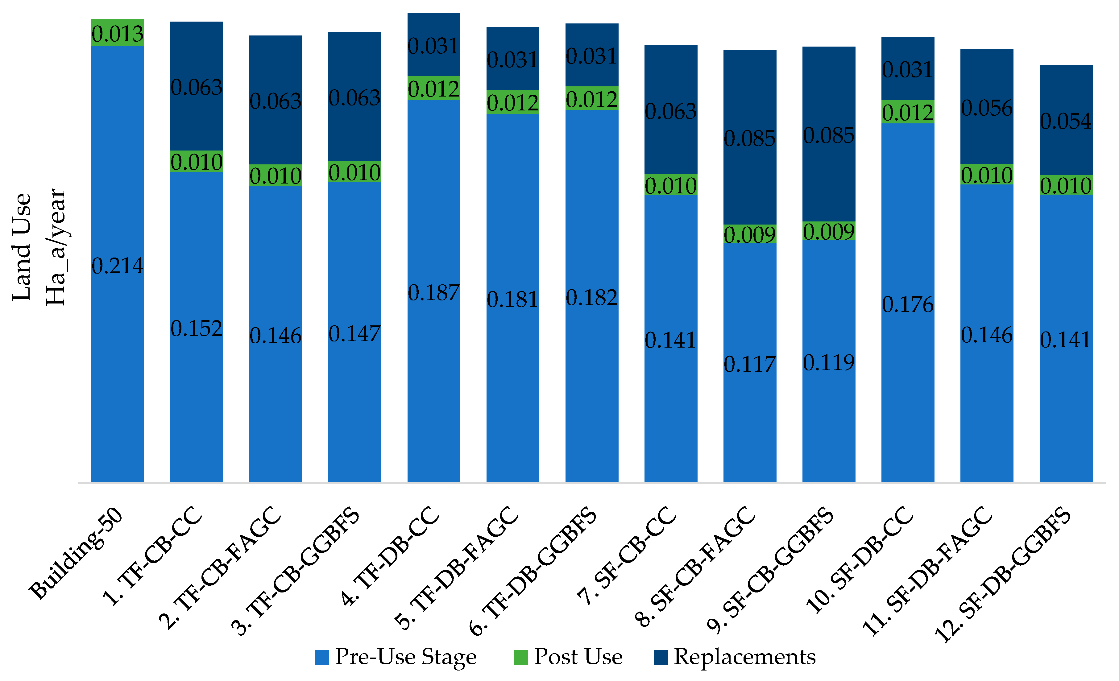
4.4. Land Use

Land use impact is the highest in the use stage (1.353 Ha_a/year) as standard energy input is used for all buildings without considering any greener choices such as wind mills, solar panels etc. The land use in the pre-use stage is the highest after the use stage as it is the summation of all land utilized during the extraction of raw materials, manufacturing of materials, transportation to site and construction equipment, followed by the replacement stage. The post-use stage land utilization is negligible as only energy consumption for the demolition and disposal of demolition waste to landfill is assessed for the study.

Figure 5 shows that the building 4 (TF-DB-CC) has the highest land use impact of 1.583 Ha_a (actual hectare) per year due to the timber frame roof (material acquired by plants) and shorter ESL. Building 12 (SF-DB-GGBFS) has the lowest impact with a value of 1.558 Ha_a/year. The longer ESL of building 12 and use of industrial by-products like GGBFS [11] has contributed to the lower land use impact.

Building 4 (TF-DB-CC), 5 (TF-DB-FAGC), and 6 (TF-DB-GGBFS) have the highest land use in the pre-use and post-use stages among 12 buildings, due to the increased amount of land requirement associated with the production of a timber frame roof, and also because these materials have short ESL meaning that more land is required to make these materials to meet the demand for replacement. The land use impact for replacement stage is higher for buildings 8 and 9 with 65-year ESL, as more energy and carbon intensive materials (e.g., ceramic tiles, rendering, plastering) requiring more space for mining, processing and manufacturing are replaced during this long ESL (Figure 2). Replaced building components in buildings 8 and 9 have about 33% to 60% of the remaining life at the end of the building service life (Figure 2).

The building with components with similar ESLs to the whole building ESL generate less waste which means the diversion of waste from landfill or residue area, thus conserving land or reducing the land footprint. From the ecological footprint point of view, the buildings with a timber roof and double brick wall frame have higher impacts than building with building components of industrial material on an annual basis, which is consistent with the existing study of Allacker et al. [73]. In the post-use stage, ceramic tiles and rendering have the highest impacts as these materials are disposed of before their ESL was finished.

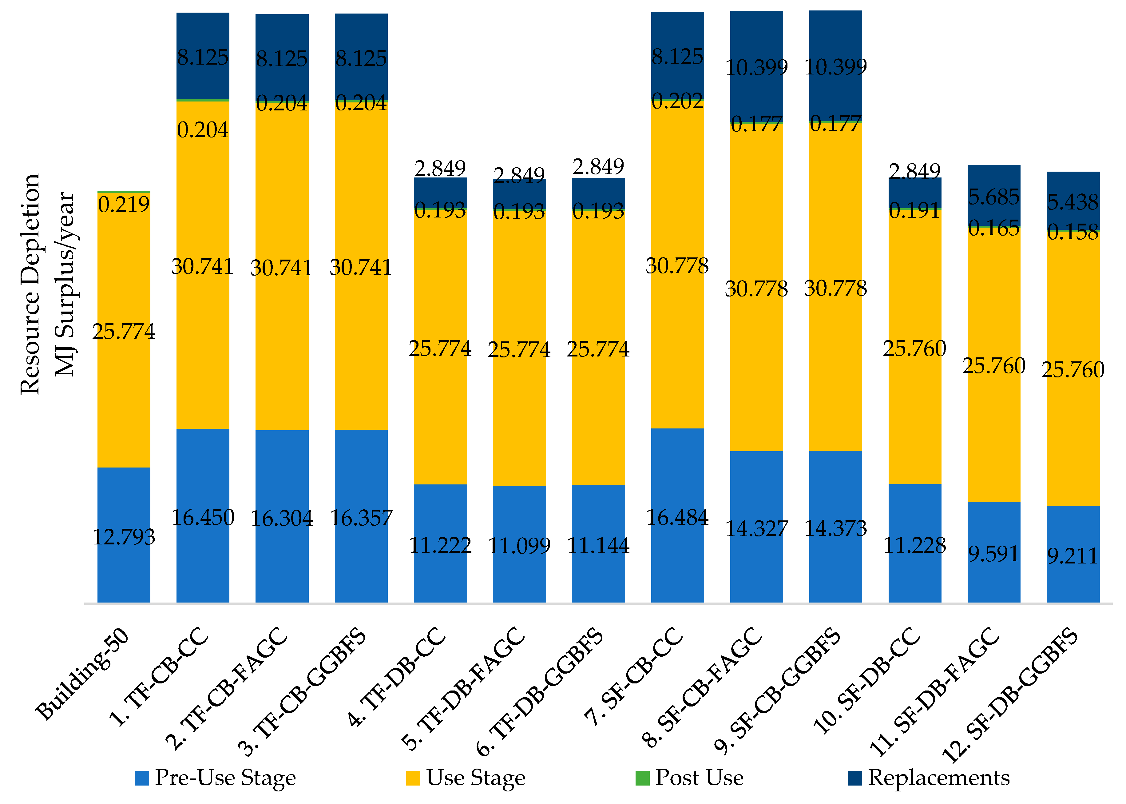
4.5. Water Consumption

Life time water consumption by case study buildings is calculated in terms of damage to resources. The resource depletion is the minimum time step to assess the water resource depletion in areas like Western Australia with fixed annual precipitation cycle [60].

Resource depletion is the highest in the use stage due to high water consumption in electricity generation [74]. The resource depletion in the pre-use stage is the second highest in buildings due to water consumption mainly in the extraction of materials and manufacturing processes. In the pre-use stage, onsite water consumption (construction works) is negligible (0.1%) as compared to upstream processing of materials. The replacement stage is contributing as the third major stage due to building component replacements. Like CED, GHG emissions and land use, the post-use stage has the least water footprint due to consideration of only demolition of buildings and transportation energy consumption to dispose of these wastes to landfill.

Figure 6 shows that the annual resource depletion is the highest for building 8 (SF-CB-GGBFS) due to use of industrial materials (steel frame, concrete block, rendering and interior plaster). The resource depletion is lowest for Building-50 as no replacement is considered for Building-50 and it has a brick wall and timber frame roof that are less water consuming materials. In the case study buildings, building 5 (TF-DB-FAGC) has slightly higher water demand as compared to the reference building (Building-50) mainly because of replacements and an ESL of 57 years.

For pre-use stages, building 7 has the highest water footprint of 16.484 MJ surplus/year due to a shorter ESL and use of building components of industrial materials. The lowest water footprint in pre-use stage is for building 12 (SF-DB-GGBFS) with longer ESL and structural components like brick, green concrete, that have lower water demand and decreased overall water consumption by building [75,76]. In concrete block wall buildings (building 1 (TF-CB-CC), 2 (TF-CB-FAGC), 3 (TF-CB-GGBFS)), water consumption in concrete block and plaster production, as well as the rendering process and their shorter ESL, are the main contributing factors for water footprint [75]. In the replacement stage, the concrete block wall and steel frame roof in buildings 8 (SF-CB-FAGC) and 9 (SF-CB-GGBFS) with 65-year ESL have the highest mineral resource depletion due to frequent replacements of rendering, interior plaster and water intensive ceramic tiles.

5. Conclusions

This study used the life cycle assessment procedure (ISO 14040-44) [38] and factor method (ISO 15686-2) [31,37], to determine the impact of service life on the environmental performance of buildings. The service life of a building and building components have a direct relationship with environmental performance of building. Estimation of replacements intervals is important in the environmental life cycle assessment of buildings, as these are the third main contributing stage to environmental impacts, after use and pre-use stage. The cumulative energy demand for building 8 (SF-CB-FAGC) is 97.779 GJ/year, 4.23% lower than the reference building, due to the ESL of 65 years. The GHG emissions for building 2 (TF-CB-FAGC) is 11.383 t CO₂ eq/year, the lowest among the case study buildings, due to use of structural components with a comparatively similar service life as ESL of buildings. The land use for building 12 (SF-DB-GGBFS) is 1.558 Ha_a, the lowest among case study buildings (0.96% lower than reference building), due to longer ESL and the use of industrial by-products which reduces land use for residue storage. Building 5 (TF-DB-FAGC) has the lowest water footprint (39.915 MJ Surplus/year) amongst case study buildings (2.827% higher than the reference building), due to use of timber and brick.

This study showed that buildings 1–12 have better performance than Building-50 for CED, and buildings 1–3, 5–9 and 11–12 have lower GHG emissions than Building-50. In the land use impact category, buildings 1–3 and 5–12 have lower land use. However, the water footprint results are slightly different than CED, GHG and land use. Building-50 has the lowest water demand as compared to the 12 case study buildings.

Current research shows that building environmental performance is dependent on building component’s materials and ESL, and the way these components are modeled into building. The use of industrial byproducts (concrete blocks, steel) could enhance performance for land use, while building materials like timber and brick have a better water footprint. Industrial byproducts (FA) have lower environmental impact for all indicators considered in this research. The service life of buildings and building components affect the environmental performance of buildings. The use of alternative, eco-friendly strategies in buildings like grey water, green concrete, renewable resources are effective only if these are aligned with building service life. Longevity of the service life of buildings can produce sustainable outcomes, if all of the building component’s service life is nearest to the building’s service life, which causes fewer replacements, as well as the GHG emissions from the transportation of waste during the post-use stage.

References

- Grant, A.; Ries, R.; Kibert, C. Life cycle assessment and service life prediction: A case study of building envelope materials. J. Ind. Ecol. 2014, 18, 187–200. [Google Scholar] [CrossRef]
- Nunen, H.V. Assessment of the Sustainability of Flexible Building: The Improved Factor Method: Service Life Prediction of Buildings in The Netherlands, Applied to Life Cycle Assessment. Ph.D. Thesis, Universiteit Eindhoven, Eindhoven, The Netherlands, 2010. [Google Scholar]
- Leticia, O.M.; Begoña, S.L. Proposed method of estimating the service life of building envelopes. J. Constr. 2015, 14, 60–88. [Google Scholar]
- Rauf, A.; Crawford, R.H. The relationship between material service life and the life cycle energy of contemporary residential buildings in Australia. Artich. Sci. Rev. 2013, 56, 252–261. [Google Scholar] [CrossRef]
- Robert, H.; Crawford, R.J.F. Energy and greenhouse gas emissions implications of alternative housing types for Australia. In Proceedings of the State of Australian Cities National Conference Australian Sustainable Cities and Regions Network (ASCRN), Melbourne, VIC, Australia, 29 November–2 December 2011; pp. 1–12. [Google Scholar]
- Robert, H.; Crawford, I.C.; Robert, J.F. A comprehensive framework for assessing the life-cycle energy of building construction assemblies. Archit. Sci. Rev. 2010, 53, 288. [Google Scholar]
- Silvestre, J.D.; Silva, A.; de Brito, J. Uncertainty modelling of service life and environmental performance to reduce risk in building design decisions. J. Civ. Eng. Manag. 2015, 21, 308–322. [Google Scholar] [CrossRef]
- Ramesh, T.; Prakash, R.; Shukla, K.K. Life cycle energy analysis of a residential building with different envelopes and climates in Indian context. Appl. Energy 2012, 89, 193–202. [Google Scholar] [CrossRef]
- Allacker, K. Sustainable Building: The Developement of an Evaluation Method. Ph.D. Thesis, Katholieke Universiteit Leuven, Leuven, Belgium, 2010. [Google Scholar]
- Audenaert, A.; de Cleyn, S.H.; Buyle, M. Lca of low energy flats using the eco-indicator 99 method: Impact of insulation materials. Energy Build. 2012, 47, 68–73. [Google Scholar] [CrossRef]
- Carre, A. A Comparative Life Cycle Assessment of Alternative Constructions of a Typical Australian House Design; PNA147-0809; Forest & Wood Products Australia: Melbourne, Australia, 2011. [Google Scholar]
- Iyer-Raniga, U.; ChewWong, J.P. Evaluation of whole life cycle assessment for heritage buildings in australia. Build. Environ. 2012, 47, 138–149. [Google Scholar] [CrossRef]
- Rouwette, R. Lca of Brick Products; Think Brick Australia: Melbourne, Australia, 2010. [Google Scholar]
- Cuellar-Franca, R.M.; Azapagic, A. Environmental impacts of the UK residential sector: Life cycle assessment of houses. Build. Environ. 2012, 54, 86–99. [Google Scholar] [CrossRef]
- Nemry, F.; Uihlein, A.; Colodel, C.M.; Wetzel, C.; Braune, A.; Wittstock, B.; Hasan, I.; Kreißig, J.; Gallon, N.; Niemeier, S.; et al. Options to reduce the environmental impacts of residential buildings in the european union-potential and costs. Energy Build. 2010, 42, 976–984. [Google Scholar] [CrossRef]
- Ortiz-Rodríguez, O.; Castells, F.; Sonnemann, G. Life cycle assessment of two dwellings: One in spain, a developed country, and one in colombia, a country under development. Sci. Total Environ. 2010, 408, 2435–2443. [Google Scholar] [CrossRef] [PubMed]
- Cabeza, L.F.; Rincón, L.; Vilariño, V.; Pérez, G.; Castell, A. Life cycle assessment (lca) and life cycle energy analysis (lcea) of buildings and the building sector: A review. Renew. Sustain. Energy Rev. 2014, 29, 394–416. [Google Scholar] [CrossRef]
- Biswas, W.K. Carbon footprint and embodied energy assessment of a civil works program in a residential estate of western australia. Int. J. Life Cycle Assess. 2014, 19, 732–744. [Google Scholar] [CrossRef]
- Islam, H.; Jollands, M.; Setunge, S. Life cycle assessment and life cycle cost implication of residential buildings—A review. Renew. Sustain. Energy Rev. 2015, 42, 129–140. [Google Scholar] [CrossRef]
- Atmaca, A. Life-cycle assessment and cost analysis of residential buildings in south east of turkey: Part 2—A case study. Int. J. Life Cycle Assess. 2016, 21, 925–942. [Google Scholar] [CrossRef]
- Lawania, K.K.; Biswas, W.K. Achieving environmentally friendly building envelope for western australia’s housing sector: A life cycle assessment approach. Int. J. Sustain. Built Environ. 2016, 5, 210–224. [Google Scholar] [CrossRef]
- Manish, K.; Dixit, J.L.F.; Lavy, S.; Charles, H.C. Need for an embodied energy measurement protocol for buildings: A review paper. Renew. Sustain. Energy Rev. 2012, 16, 3730–3743. [Google Scholar]
- Vitale Pierluca, A.N.; Fabrizio, D.G.; Umberto, A. Life cycle assessment of the end of life phase of a residential building. Waste Manag. 2017, 60, 311–321. [Google Scholar] [CrossRef]
- Pierluca Vitale, U.A. An attributional life cycle assessment for an italian residential multifamily building. Environ. Technol. 2018, 39, 3033–3045. [Google Scholar] [CrossRef]
- Balasbaneh, A.T.; Marsono, A.K.B.; Khaleghi, S.J. Sustainability choice of different hybrid timber structure for low medium cost single-story residential building: Environmental, economic and social assessment. J. Build. Eng. 2018, 20, 235–247. [Google Scholar] [CrossRef]
- Buildings and constructed assets—Service life planning. Part-1: General Principles and Framework; ISO 15686-1; International Standards Organisation: Geneva, Switzerland, 2011. [Google Scholar]
- Hed, G. Service life planning of building components. Durab. Build. Mater. Compnt. 1999, 8, 1543–1551. [Google Scholar]
- Hovde, P.J.; Moser, K. Performance Based Methods for Service Life Prediction; In-House Publishing: Rotterdam, The Netherlands, 2004. [Google Scholar]
- Masters, L.W.; Brandt, E. Prediction of service life of building materials and components. Mater. Struct. 1987, 20, 55–77. [Google Scholar] [CrossRef]
- Building and constructed assets—Service planning. Part 1: General Principals and Framework; ISO 15686-1:2000; International Standards Organisation: Geneva, Switzerland, 2000. [Google Scholar]
- Buildings and constructed assets—Service life planning. Part-2: Service Life Prediction Procedures; ISO 15686-2; International Standards Organisation: Geneva, Switzerland, 2012. [Google Scholar]
- Cecconi, F. Performance lead the way to service life prediction. In Proceedings of the 9th International Conference on Durability of Building Materials and Components, Brisbane, Australia, 17–20 March 2002. [Google Scholar]
- Ivan Cole, P.C. Predicting the service life of buildings and components. Constr. Mater. 2011, 164, 305–314. [Google Scholar] [CrossRef]
- Chen, C.-J.; Juan, Y.-K.; Hsu, Y.-H. Developing a systematic approach to evaluate and predict building service life. J. Civ. Eng. Manag. 2017, 23, 890–901. [Google Scholar] [CrossRef]
- Hovde, P.J. Performance Based Methods for Service Life Prediction, Part A: Factor Methods for Service Life Prediction. Available online: http://site.cibworld.nl/dl/publications/Pub294.pdf (accessed on 1 January 2019).
- Hovde, P.J. Evaluation of the Factor Method to Estimate the Service Life of Building Components; Department of Building and Construction Engineering, The Norwegian University of Science and Technology: Trondheim, Norway, 1998. [Google Scholar]
- Buildings and constructed assets—Service-life planning. Part 8: Reference Service Life and Service-Life Estimation; ISO 15686-8; International Standards Organisation: Geneva, Switzerland, 2008. [Google Scholar]
- Environmental Management—Life Cycle Assessment, Principles and Framework; ISO 14040; International Standards Organization: Geneva, Switzerland, 2006.
- Guinee, J.B.; Udo de Haes, H.A.; Huppes, G. Quantitative life cycle assessment of products: 1: Goal definition and inventory. J. Clean. Prod. 1993, 1, 3–13. [Google Scholar] [CrossRef]
- Consoli, F.A.; Boustead, I.; Fava, J.; Franklin, W.; Jensen, A.; Oude, N.; Parrish, R.; Perriman, R.; Postlethwaite, D.; Quay, B.; et al. Guide Lines for Life-Cycle Assessment: A Code of Practice; Society of Environmental Toxicology and Chemistry: Pensacola, FL, USA, 1993. [Google Scholar]
- Bekker, P.C.F. A life cycle approach in building. Build. Environ. 1982, 17, 3–13. [Google Scholar] [CrossRef]
- Ortiz, O.; Castells, F.; Sonnemann, G. Sustainability in the construction industry: A review of recent developments based on lca. Constr. Build. Mater. 2009, 23, 28–39. [Google Scholar] [CrossRef]
- Lotteau, M.; Loubet, P.; Pousse, M.; Dufrasnes, E.; Sonnemann, G. Critical review of life cycle assessment (lca) for the built environment at the neighborhood scale. Build. Environ. 2015, 93, 165–178. [Google Scholar] [CrossRef]
- Anderson, J.E.; Wulfhorst, G.; Lang, W. Expanding the use of life-cycle assessment to capture induced impacts in the built environment. Build. Environ. 2015, 94, 403–416. [Google Scholar] [CrossRef] [Green Version]
- Passer, A.; Ouellet-Plamondon, C.; Keneally, P.; John, V.; Habert, G. Impact of future scenarios on building renovation strategies towards plus energy buildings. SBE16 Zurich 2016, 124, 2. [Google Scholar]
- Norman, J.; MacLean, H.; Kennedy, C.A. Comparing high and low residential density: Life-cycle analysis of energy use and greenhouse gas emissions. J. Urban Plan. Dev. 2006, 132, 10–21. [Google Scholar] [CrossRef]
- Wahidul, K.; Biswasa, Y.A.; Krishna, K.L.; Prabir, K.S.; Elsarrag, E. Life cycle assessment for environmental product declaration of concrete in the gulf states. Sustain. Cities Soc. 2017, 35, 36–46. [Google Scholar]
- Lawania, K.K.; Biswas, W.K. Cost-effective ghg mitigation strategies for western australia’s housing sector: A life cycle management approach. Clean Technol. Environ. Policy 2016, 18, 2419–2428. [Google Scholar] [CrossRef]
- Werner, F.; Richter, K. Wooden building products in comparative lca. Int. J. Life Cycle Assess. 2007, 12, 470–479. [Google Scholar]
- Wahidul, K.; Biswas, L.B.; Carter, D. Global warming potential of wheat production western australia: A life cycle assessment. Water Environ. J. 2008, 22, 206–216. [Google Scholar]
- Mirabella, N.; Röck, M.; Saade, M.R.M.; Spirinckx, C.; Bosmans, M.; Allacker, K.; Passer, A. Strategies to improve the energy performance of buildings: A review of their life cycle impact. Buildings 2018, 8, 105. [Google Scholar] [CrossRef]
- Vincenzo Franzitta, M.L.; Gennusa, G.P.; Rizzo, G.; Scaccianoce, G. Toward a european eco-label brand for residential buildings: Holistic or by-components approaches? Energy 2011, 36, 1884–1892. [Google Scholar] [CrossRef]
- Francesco Barreca, P.P. Post-occupancy evaluation of buildings for sustainable agri-food production—A method applied to an olive oil mill. Buidings 2018, 8, 83. [Google Scholar] [CrossRef]
- Samaratunga, M.; Ding, L.; Bishop, K.; Prasad, D.; Yee, K.W.K. Modelling and Analysis of Post-Occupancy Behaviour in Residential Buildings to Inform Basix Sustainability Assessments in Nsw. Procedia Eng. 2017, 180, 343–355. [Google Scholar] [CrossRef]
- Aneurin Grant, R.R. Impact of building service life models on life cycle assessment. Build. Res. Inf. 2013, 41, 168–186. [Google Scholar] [CrossRef]
- Galle, W.; de Temmerman, N.; de Meyer, R. Integrating scenarios into life cycle assessment: Understanding the value and financial feasibility of a demountable building. Buidings 2017, 7, 64. [Google Scholar] [CrossRef]
- TCI. Australia’s Emissions: What Do the Numbers Really Mean? The Climate Institute: Sydney Australia, 2015. [Google Scholar]
- Argent, R.M. Australia State of the Environment 2016: Inland Water; Australian Government Department of the Environment and Energy: Canberra, Australia, 2017. [Google Scholar]
- BOM. Average Anual, Seasonal and Monthly Rainfall; BOM: Melbourne, Australia, 2018. [Google Scholar]
- Pfister, S.; Koehler, A.; Hellweg, S. Assessing the environmental impacts of freshwater consumption in lca. Environ. Sci. Technol. 2009, 43, 4098–4104. [Google Scholar] [CrossRef] [PubMed]
- Fenton, G.G. Desalination in australia-past and future. Desalination 1981, 39, 399–411. [Google Scholar] [CrossRef]
- Radcliffe, J.C. The water energy nexus in australia-the outcome of two crises. Water-Energy Nexus 2018, 1, 66–85. [Google Scholar] [CrossRef]
- Joe Pickin, P.R. Australian National Waste Report 2016; Department of the Environment and Energy & Blue Environment Pty Ltd.: Docklands, Australia, 2017. [Google Scholar]
- PRe’-Consultants. Simapro 8.4 Lca Software; Pre’ Consultants: Amersfoort, The Netherlands, 2016. [Google Scholar]
- Shahana, Y.; Janjua, P.K.S.; Wahidul, K.B. Sustainability implication of a residential building using a lifecycle assessment approach. In Proceedings of the 4th International Conference on Low Carbon Asia and Beyond (ICLCA), Johor Bahru, Malaysia, 24–26 October 2018; Chemical Engineering Transactions: Johor Bahru, Malaysia, 2018; Volume 73, pp. 1–6. [Google Scholar]
- AccuRate. Accurate Sustainability Tool Version 2.3.3.13 sp3; CSIRO Land & Water Flagship and Distributed by Energy Inspection Pty Ltd.: Canberra, Austrailia, 2015. [Google Scholar]
- Crowther, P. Design for disassembly to recover embodied energy. In Proceedings of the 16th International conference on Passive and Low Energy Architecture, Melbourne/Brisbane/Cairns, Australia, 22–24 September 1999. [Google Scholar]
- Lawania, K.K. Improving the Sustainability Performance of Western Australian House Construction: A Life Cycle Management Approach; Curtin University: Perth, Australia, 2016. [Google Scholar]
- Treloar, G.; Fay, R.; Love, P.E.D.; Iyer-Raniga, U. Analysing the life-cycle energy of an australian residential building and its householders. Build. Res. Inf. 2000, 28, 184–195. [Google Scholar] [CrossRef]
- Fay, R.; Treloar, G.; Iyer-Raniga, U. Life-cycle energy analysis of buildings: A case study. Build. Res. Inf. 2000, 28, 31–41. [Google Scholar] [CrossRef]
- Vass, N. Western Australia Energy Fact Sheet. Available online: http://www.australianpowerproject.com.au/western-australia-energy-fact-sheet/ (accessed on 19 December 2018).
- Lawania, K.; Biswas, W.K. Application of life cycle assessment approach to deliver low carbon houses at regional level in western australia. Int. J. Life Cycle Assess. 2018, 23, 204–224. [Google Scholar] [CrossRef]
- Allacker, K.; Maia de Souza, D.; Sala, S. Land use impact assessment in the construction sector: An analysis of lcia models and case study application. Int. J. Life Cycle Assess. 2014, 19, 1799–1809. [Google Scholar] [CrossRef]
- Spang, E.S.; Moomaw, W.R.; Gallagher, K.S.; Kirshen, P.H.; Marks, D.H. The water consumption of energy production: An international comparison. Environ. Res. Lett. 2014, 9, 1–14. [Google Scholar] [CrossRef]
- Bardhan, S. Assessment of water resource consumption in building construction in India. WIT Trans. Ecol. Environ. 2011, 144, 93–101. [Google Scholar] [Green Version]
- Robert, H.G.; Treloar, J.T. An assessment of the energy and water embodied in commercial building construction. In Proceedings of the 4th Australian Life Cycle Assessment Conference, Sydney, NSW, Australia, 23–25 February 2005; pp. 1–10. [Google Scholar]
Figure 1.
Building environmental performance assessment procedure.
Figure 2.
Remaining service life of building components at Post-Use Stage.
Figure 3.
Cumulative Energy Demand per year per building, for 12 buildings and Building-50. (Use stage is omitted in the graph as the use-stage CED value 82.634 GJ/year is uniform in all cases and if plotted on same scale, other stages due to low values cannot be presented properly).
Figure 4.
Life cycle greenhouse gas (GHG) emissions per year per building for 12 buildings and Building-50. (Use stage is omitted in the graph as the use-stage GHG value 9.918 t CO2 eq/year is uniform in all cases and if plotted on same scale, other stages due to low values cannot be presented properly).
Figure 5.
Life cycle land use per year per building for 12 buildings and Building-50. (Use stage is omitted in the graph as the use-stage Land use value 1.353 Ha_a/year is uniform in all cases and if plotted on same scale, other stages due to low values cannot be presented properly).
Figure 6.
Life cycle resource depletion per year per building for 12 buildings and Building-50.