Impact of Heat Pump Flexibility in a French Residential Eco-District


1
University Grenoble Alpes, CNRS, Grenoble INP, G2Elab, 38000 Grenoble, France
2
Gaz et Electricité de Grenoble, 57 Rue Pierre Semard, 38000 Grenoble, France
*
Author to whom correspondence should be addressed.
Buildings 2018, 8(10), 145; https://doi.org/10.3390/buildings8100145
Submission received: 23 August 2018
/
Revised: 26 September 2018
/
Accepted: 17 October 2018
/
Published: 19 October 2018
(This article belongs to the Special Issue Environmental Impact Assessment of Buildings)
Abstract
:This paper investigates the impact of load shedding strategies on a block of multiple buildings. It particularly deals with the quantification of the factors i.e., peak shaving, occupants’ thermal comfort or CO emission reduction and how to quickly quantify them. To achieve this goal, the paper focuses on a new residential district, thermally fed by heat pumps. Four modeling approaches were implemented in order to estimate buildings’ response towards load shedding. Two schemes were combined in order to study an overall load shedding. This strategy for the neighborhood has proved itself efficient for both peak shaving and thermal comfort. Most of the clipped heating load during the peak period is shifted to low-consumption periods, providing an effective peak shaving. The thermal comfort is guaranteed for at least 96% of the time. For CO emissions reduction, the link between consumption reduction and CO emissions savings should be realized carefully, since shifting the consumption could increase these emissions.
1. Introduction
1.1. Background
Within three years of the 21st United Nations Climate Change Conference (COP21), a number of energy transition policies have been carried out in order to respect the Paris Agreement in keeping the global average temperature below 2 °C of pre-industrial levels [1]. The massive integration of renewable energy sources, together with the electrical peak consumption augmentation put load flexibility in a central position in regards to energy transition strategies, as it could help to guarantee grid stability [2].
Many new stakeholders, as well as new markets, appear in order to modulate electrical consumption [3]. However, aggregators mostly apply these demand response strategies on electricity-intensive industries, excluding lower power level sites such as buildings. Nevertheless, the latter represents a large share of global energy consumption. Owing to their thermal inertia, different load shedding schemes (recurring or non-recurring) can be implemented on the buildings; yet the flexibility of these schemes is hard to evaluate quickly.
Therefore, it became one of the key points studied in the European project City-zen [4]. Our collaborative effort with the local Distribution System Operator (DSO), Grenoble Electricity and Gas (GEG), takes place in this context and focuses on a new residential eco-district. This district consists of 23 residential buildings having 264 apartments and is thermally fed by ground source heat pumps (GSHP); thus emphasizing the primary use of electrical energy for heating purposes. Indeed, GSHP represent a significant research field [5,6], so that they are at the cutting edges of research with the demand side management (DSM) in order to manage electric grid constraints [7].
1.2. Literature Review
On the one hand, peak-shaving strategies are widely studied in order to deal with electric grid constraints [8]. On the other hand, DSM becomes more studied at a local scale [9], focusing on local energy integration [10], demand curve smoothing [11] or economic purposes [12]. These two combined lead to an increase of research papers on the field of peak-shaving for better management of local electric grid constraints through DSM [13].
The idea of using buildings’ thermal inertia in order to modulate the heating load is also vastly studied. While buildings’ flexibility is studied with several aims such as increasing district heating efficiency [14,15] or for a better integration of local production sources [16], it is also investigated with the objective to evaluate what could be their future impact in smartgrids [17] and to compare them to storage solutions [18]. Several methodologies have been developed in order to quantify this flexibility but only three are commonly applied using building structural mass [19]. Moreover, only a few of these papers evaluate the impact on thermal comfort as they mostly consider it as a constraint [20]. In our case, the possibility to be out of the comfort zones will be considered, usually defined by set-point temperature ranges [18,21], while estimating this impact by standing on comfort ranges as defined in [22].
Most of the time, estimating the building temperature is possible as the building thermal flexibility quantification is based on thermal models. These models can be from low-order RC models [23] to higher-detailed models often based on widespread tools such as EnergyPlus [18,24] or based on the Modelica language such as the library IDEAS [25]. Even the district scale becomes more and more widespread in the energetic dynamic simulation software, like DIstrict MOdeller and SIMulator (DIMOSIM) developed by CSTB [26], City Energy Analyst (CEA) developed by ETH Zurich [27] or Tool for Energy Analysis and Simulation for Efficient Retrofit (TEASER) developed by RWTH Aachen [28]. It was observed that this scale change could be impractical by being relevant to annual heating needs, but not anymore when focusing on power analysis [29]. For this reason, models with different levels of detail have been studied.
1.3. Context and Aims of the Study
In the local context of Grenoble, an electrical consumption peak appears between 5 a.m. and 10 a.m. GEG is interested in peak shaving during this morning period by implementing effective load shedding scheme. However, it could be hard to quickly quantify the impact of load shedding strategies through peak shaving while avoiding thermal discomfort for occupants and an increase in carbon footprint simultaneously.
Indeed, the problem is complex to model. In order to maintain occupants’ thermal comfort, load shedding can be realized after an over-heating so that the building could store heat before disconnecting the heating system. As it induces an over-consumption, this over-heating should be performed before the peak period (i.e., between 5 a.m. and 10 a.m. in our case), with the purpose of reducing the consumption peak. In order to study a strategy of district peak reduction by deliberate load shedding building by building, two load shedding strategies (with or without over-heating) will be compared.
This paper aims to quickly quantify the influence of this district heat load shedding strategy on the heat load curve, thermal comfort and greenhouse gases emissions reduction. Moreover, the study will try to quantify the impact of heat load profiles modeling on the results.
1.4. Paper Structure
The first section of this paper describes the methods used for load shedding impact quantification. At first, the impact indicators in terms of peak shaving, thermal comfort and CO reduction will be defined. Then, the heat load profiles modeling will be presented. Finally, the load shedding scenarios studied in the paper will be introduced. In the ‘Results’ section, the two load shedding strategies will be analyzed on a building with respect to the indicators introduced earlier. The results will show the impact on three aspects: peak-shaving, thermal comfort, and CO emissions while analyzing the effect of the heat load profiles modeling. A conclusion will be drawn at the end of the paper based on the observed results.
2. Methods for Impact Quantification of Load Shedding
2.1. Indicators for Impact Quantification of Load Shedding
2.1.1. Peak Shaving
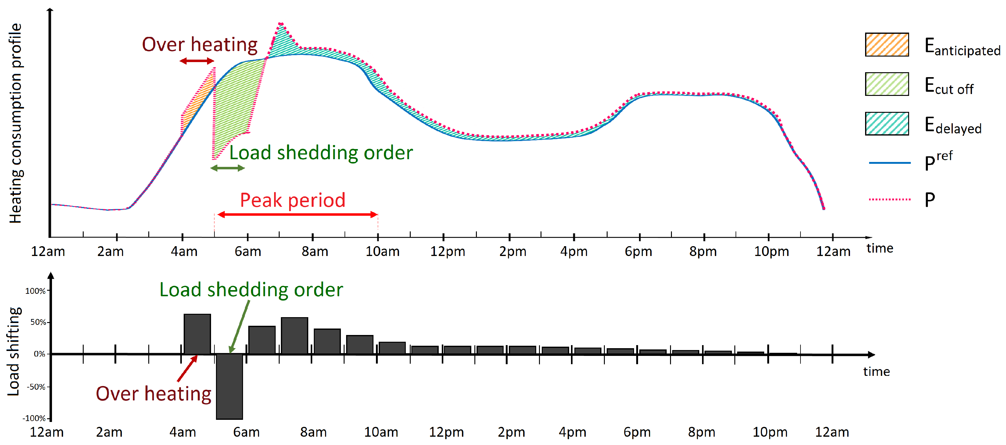
In order to quantify the amount of load reduction in a district, the key indicators will be defined first. Many studies show some rebound effects after a load shedding, related to the restart of the consumption [30]. This behavior could not only affect the energy conservation by providing any (or few) consumption reductions at a daily scale, but it could also lead to failure of peak shaving strategy. Indeed, if concentrated during a short period, a load shifting could cause bigger grid constraints during this time period. For this reason, in order to quantify the impact of load shedding strategies for peak shaving purpose, the consumption behaviour after the load shedding period has to be analyzed. To do so, the study is based on one indicator used by the French TSO RTE [31] (cf. Equations (1)–(4) and (8)). The daily Load Shifting rate (LS)) is defined in Equation (1) from the ratio of the addition of anticipated energy and delayed energy, by the cut-off energy. These three energies are defined in Equations (2)–(4) by the integral in a given period of the consumption power (P) and its reference value without operation (P). These energies are also visible in Figure 1.
where:
By taking into account the energy reported during the 23 h following the load shedding, this indicator gives information at a daily scale. However, in order to get a better understanding of the dynamic behavior of this energy report, the study will rather focus on an adapted form of this load shifting rate, that we proposed, defined in Equation (5). This indicator will be calculated on an hourly basis in order to quantify the distribution of energy report, hour by hour, as shown in Figure 1.
Defined as such, the load shifting rate can be used to study dynamically the load variations and gives information on the efficiency of the load shedding strategy to reduce a long peak period (more than one hour).
2.1.2. Thermal Comfort
It is important to keep in mind that turning off the heat supply can affect the thermal comfort so that this aspect has to be estimated too. When the thermal supply of a building is turned off, the internal temperature does not decrease instantaneously to the level of external temperature. This building dynamic can be explained by the possibility for buildings to store heat in their heavy components, such as walls. Indeed, due to their significant inertia, walls will cool later than the air, in cases of heating load shedding. The phenomena are important in terms of comfort, as walls and air temperatures respectively reflect radiation and convection effects perceived by the occupants of the building. Since the feeling of thermal comfort is related to this perception of both air and wall temperature, studies analyzed the relationship between thermal comfort and the operative temperature (T, defined Equation (6)) [32].
In this study, this operative temperature will be taken as an indicator in order to estimate the comfort level, according to levels defined in [22]:
- Comfortable: A range of +/− 1 °C about the temperature set-point (T)
- Slightly uncomfortable: A range of +/− 1 °C and +/− 2 °C about T
- Uncomfortable: A difference of more than 2 °C with T
2.1.3. CO Emissions Reduction
Finally, the impact of the different load shedding methods on CO emissions will be studied. To do so, the work will rely on the actual CO emissions from the French power generation in January 2016 [33]. This will allow us to estimate the gross CO emissions variation when the load shedding strategies will be applied while taking into account hourly and daily variation (see Equation (7)).
This variation not only takes into account the load shifting, but also the consumption reduction. Moreover, it is very common to conclude that CO emissions will obviously decrease with load shedding strategies when there is energy saving. A widespread indicator for energy saving [31] is the daily Energy Saving rate (ES) defined as follows:
This energy saving rate is commonly used to quantify energy balance in the long-run by showing the amount of non-reported energy 23 h after [31]. The energy saving rate should be put into perspective, as it represents saving in regard to cut-off energy. Since the energy saving of an entire day is much lower than ES, the reduction of daily CO emissions would be lowered too.
Nevertheless, this does not prevent us from expecting that CO emissions would decrease as much as daily consumption. To deeply examine the impact on district carbon footprint, it is crucial to consider the daily and intra-day CO emission variability for the electrical energy generation. Shifting the electrical consumption from one time period to another could increase the CO emissions if local peaks do not match the total electricity generation.
For all these reasons, the paper will compare the total consumption reduction (ES) to the total CO emissions reduction during the month (COS). Doing this will help us in combining the two reduction factors (energy consumption and CO emissions) into a single indicator, the Expected Gain reduction (EG), defined as follows:
2.2. Heat Load Profiles Models
According to the previously defined indicators, the thermal load variation between no-load shedding and the applied load shedding strategy need to be assessed in order to quantify the impact on peak shaving and CO emissions. In the present study, two modeling approaches will be compared. At first, a standard load shifting profile will be established with experimental data. Then, thermal models with several levels of details will be introduced in order to assess thermal comfort.
2.2.1. Experimental Load Shifting Profile
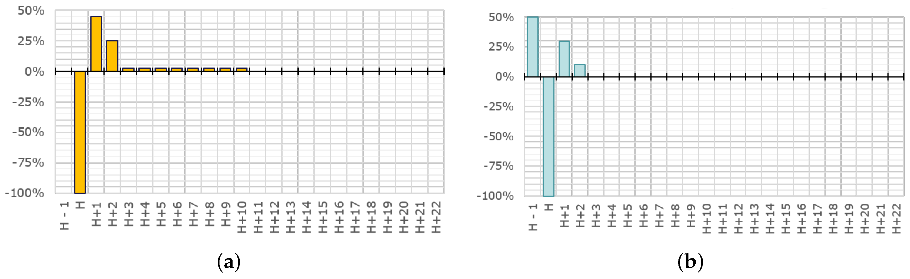
A first estimation can rely on experimental results from similar buildings and load shedding strategies. The main advantage of this method is to assess very quickly the peak shaving indicator. To do so, a standard load shifting rate profile was defined, based on experimental results from the French GreenLys project [34] and from a study led by the French TSO RTE [31]. As the experimental building stock contains two new eco-districts [34], the use of the resulting standard profile is considered suitable for our new residential district. The experimental results show an energy saving rate around 90%. The load shifting rate profiles are plotted below.
2.2.2. Thermal Models
In order to quantify the impact on thermal comfort, it is also necessary to estimate T (cf. Equation (6)). For this reason, two thermal models with identified parameters were used in order to simulate the building dynamic during and after the load shedding.
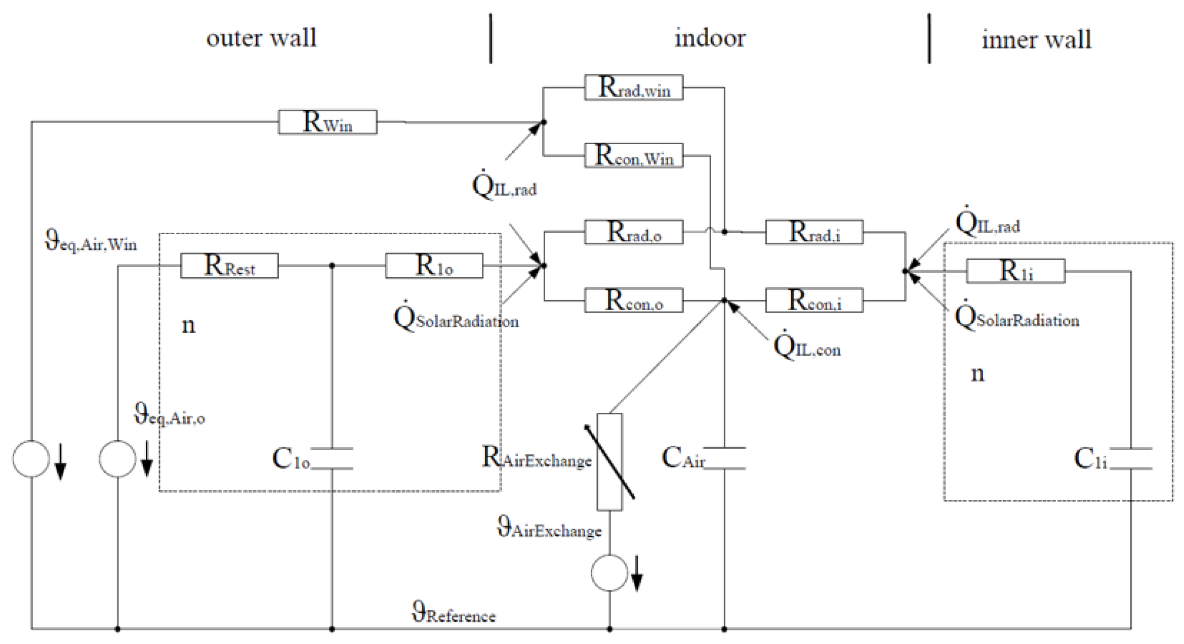
In order to manage both modelings (thermal model of the building and electric model of the grid), an open-source tool, TEASER [35] was chosen for the first thermal model creation. It allows to automatically generate RC thermal models in the Modelica language for the AixLib [36] and the Annex60 [37] libraries.
The thermal model can be created thanks to building envelope information (wall areas, orientations, thickness, materials, etc.). As it can be difficult to access the specific data about each building envelope at district level, it can be realized with at least 5 input data: year of construction, net area, type of use, number of floors and height of each floor [35], making the tool very useful for saving time. If only this data is given, the tool enriches the dataset based on pre-defined statistical data, whose use in a French context will be analyzed in this study case.
For the same thermal model structure (see Figure 3), two precision levels can be achieved depending on the input data. In order to compare the impact of dataset enrichment, both the model generated with the 5 minimal parameters and the model enriched with the building envelope data were analyzed. The first one will further be referred to as the ’Simple’ model, while the second one enriched with data used for the regulatory Building Energy Simulation (BES) will further be referred to as the ’Enriched’ model.
The second one is the fully detailed thermal model used for the mandatory study. Indeed, in a French context, since each building construction requires an energy requirement study based on a fully detailed thermal model, existing thermal models from this mandatory study can also be re-used. In this study, a Pleiades tool [38] has been used to build a detailed model (each room is considered as a thermal zone), that will be called ’Complex’ model afterward.
For all heat load profiles from simulation models, the result from a thermal dynamic simulation of a building in our district was considered as reference heat load profile (P). The building behavior in the case of a temperature set-point of 20 °C was simulated during the month of January. All other data: weather, occupancy schedules, internal gains for lightning etc. have been set to the same values in order to obtain a better comparison between simulation results. However, the set-point temperatures for the ’Simple’ and ’Enriched’ models are ambient temperatures, while the one in ’Complex’ model is on the operative temperature, and cannot be changed. Therefore, small differences between the results could still be expected.
2.2.3. Summary of Modeling Approaches
To summarize, four modeling approaches are considered in order to estimate the load shifting rates is this paper:
- The ‘Standard’ model: the statistical model from experimental data
- The ‘Simple’ model: thermal model generated by TEASER (Figure 3) with database
- The ‘Enriched’ model: thermal model generated by TEASER (Figure 3) with building envelope data
- The ‘Complex’ model: multi-zone thermal model created with a Pleiades tool.
2.3. Modeling of Load Shedding Scenarios
For the aforementioned models, two scenarios will be studied:
- One-hour thermal load shedding after one-hour over-heating: In order to over-heat the building outside of the peak period (5 a.m. to 10 a.m.), the load shedding order will be applied from 5 a.m. to 6 a.m.
- Simple one-hour thermal load shedding: In this scenario, the load shedding will be applied in the middle of the peak period, from 7 a.m. to 8 a.m. without any over-heating.
Each load shedding will be obtained by a very low set-point temperature (around 0 °C) in order to cut the heat supply. The aim of these two scenarios is to represent the two load shedding approaches that could be made building by building in the district. For instance, by applying the first strategy (with over-heating) to a first building and then applying the second strategy to each of the four other buildings hour by hour, the resulting load shedding on the entire district would be obtained by adding the individual effects (see Figure 4).
3. Results and Discussion
The load shedding impact in terms of peak shaving, thermal comfort and CO emissions will be analyzed in this section. As explained previously, the district load-shedding strategy consists in shedding thermal load for the buildings one by one for one hour. The first load shedding would integrate a one-hour over-heating during the previous hour, while all the following hours will face simple one-hour thermal load shedding. Two different building behaviors are thus expected for these two strategies.
3.1. Results for Peak Shaving
In order to reduce the mean power during the peak period, the load shifting rate would have to be the most diffused as possible to shift most of the consumption out of the peak period. Thus, the lower load shifting rates are, the higher the efficiency of peak shaving. As two dynamic responses are expected from the building depending on whether it has been previously over-heated or not, results will be demonstrated for both load shedding strategies. At first, results for a simple thermal load shedding happening from 7 a.m. to 8 a.m. each day of the month of January will be drawn. Then, the second load shedding strategy with a one-hour over-heating before cutting the heat supply will be shown. This load shedding will be applied from 5 a.m. to 6 a.m., in order to shift the anticipated consumption before the peak period.
3.1.1. Thermal Load Shedding from 7 a.m. to 8 a.m.
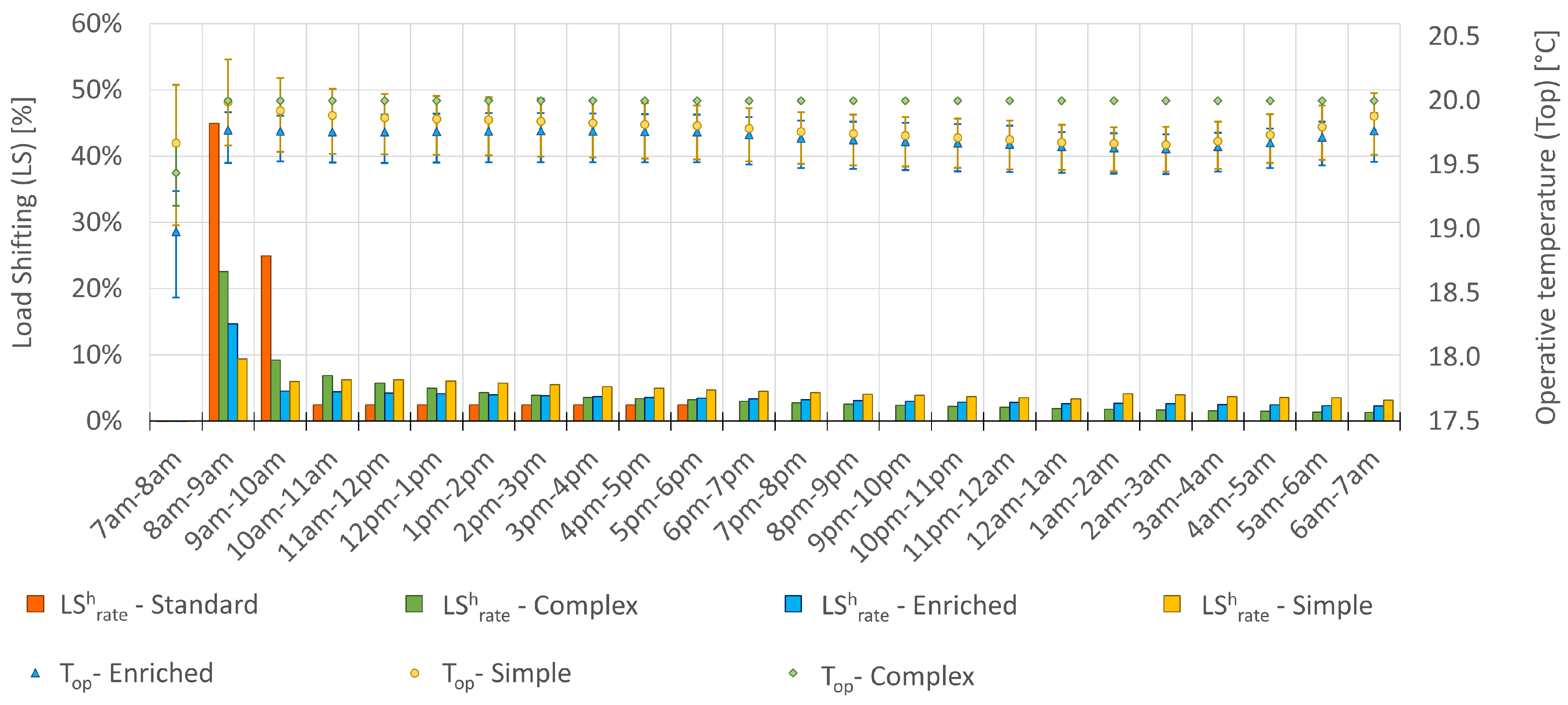
The results of the simple one-hour load shedding applied all days of January are displayed in Figure 5. The mean load shifting can be found for all of the four modeling approaches (‘Standard’, ‘Simple’, ‘Enriched’ and ‘Complex’). The mean operative temperatures are also drawn with their variation range during the month.
Two different building behaviors can be observed for this strategy:
- Most of the rebound effect appears within the two hours following the load shedding (experimental load shifting profile)
- The shed consumption is shifted during the entire day (load shifting profiles from thermal models)
Here, it can be noticed that all the simulation results from thermal models show a slower dynamic than the experimental load shifting profile.
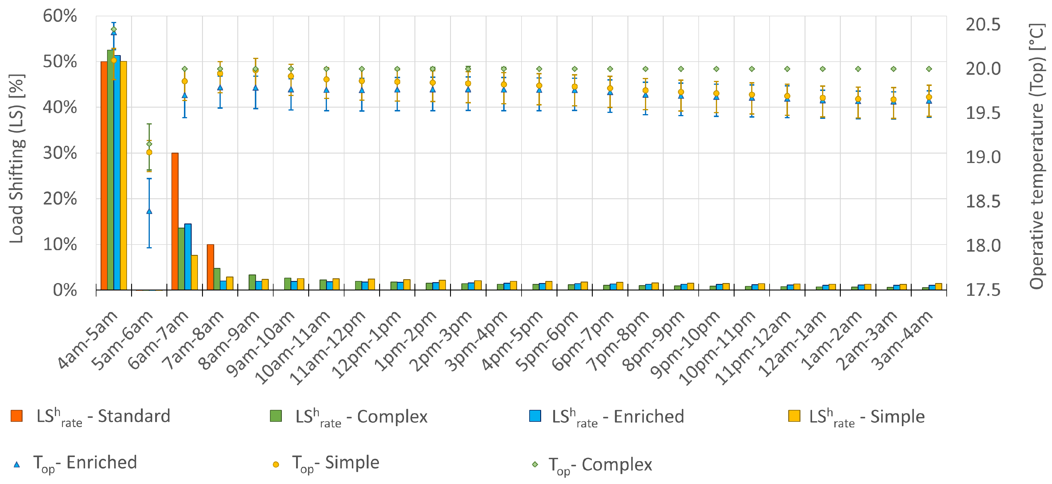
3.1.2. Heat Load Shedding from 5 a.m. to 6 a.m. after an Over-Heating in Preceding Hour
The results of the complex one-hour thermal load shedding strategy, taking place from 5 a.m. to 6 a.m. after a one-hour over-heating are presented in Figure 6. The strategy was applied each day of January and results are the average value for each time slot and each modeling, like those presented in Figure 5. As seen before, there is a big difference between experimental and simulated buildings behaviors for simple heat load shedding strategy. This gap between models is therefore confirmed for this complex strategy too.
Although this standard profile was established from real measurement, it remains difficult to consider it as more reliable than simulated profiles. Indeed, weather and occupancy data differ and several types of buildings are aggregated. Even with fewer old buildings than new ones in the experiment, consumption values for heating tend to be higher for the first category and mean values could be strongly affected. In spite of this conclusion, the standard model reminds that occupancy behavior could play a great role in the rebound effect. In our study case, the thermal load is entirely controlled by the building manager, so this effect can be neglected.
Thus, conclusions on the effect of the overall strategy (starting with the complex strategy and continuing, building by building, with the simple load shedding) could be realized by analyzing the building behaviors predicted by thermal models. These three modeling approaches all lead to diffused energy reports so that it can be concluded that this load shedding strategy could be efficient in regards to a peak shaving objective, even if thermal comfort still needs to be looked at.
3.2. Results for Thermal Comfort
As explained above, the study focuses on the building operative temperature as thermal comfort indicator. With a set-point temperature fixed to 20 °C, the comfort zone is reached over 19 °C and below 21 °C. Results obtained for the month of January are presented in Figure 5 and Figure 6. Mean operative temperatures are represented, with their variation intervals, so that it can be noticed that:
- On average, load shedding hours are slightly uncomfortable
- On average, other hours of the days are comfortable
Distribution of comfort level for occupants for the load shedding strategy after an over-heating is presented in Table 1:
Similar results are obtained for the load shedding strategy without over-heating. Most of the hours are “comfortable” (at least 96% of the time for all models) and “uncomfortable” level is rarely reached (0.4% of the time and only with the ‘Enriched’ model). However, further studies on the impact of heating systems (as shown in [16]) or on the perception of this comfort could be needed to consolidate these results (as studied in [39]). As internal gains and external temperatures differ each hour, each time slot should be considered individually for further studies in the entire district impact. Finally, requiring less energy for heating purposes, new low-consumption buildings could get a large part of their heating needs from internal gains (lightning, devices, occupation, etc.). This would also have to be considered carefully in order to avoid an under-evaluation of thermal discomfort in buildings.
3.3. Results for CO Emissions Reduction
In this last section, the results for the impact on the carbon footprint are presented. The chosen indicator for the effect is the expected gain reduction (EG), representing the difference between CO emission reduction expected by looking at the energy consumption savings (ES) and the effective CO emission diminution (COS). In order to put into perspective the feeling of savings obtained by looking at the mean ES, the following Table 2 will also integrate it in comparison to the effective consumption reduction during the month (ES).
For the load shedding between 7 a.m. and 8 a.m. (simple load shedding), the intuition is confirmed since the overall consumption reduction leads to the reduction of the CO emission, though a little less than expected. However, for the second strategy with overheating, reduction of CO emission is not so obvious anymore. Depending on the models, the expected CO emission reduction is lower than the calculated one. It goes from 76% less than expected to an increase of 44% of CO emissions. In terms of avoided CO emissions, the savings go from 245 g (CO = 0.01%) to 7.82 kg (CO = 0.38%) The reason for these differences is that the load is transferred from a low-CO emissions time slot to higher CO emissions times of the day. In order to be consistent with energy transition strategies, it is important to consider this aspect into load shedding impact evaluation to avoid a local amelioration to the detriment of general interest.
4. Conclusions
With often few data available at the district level, thermal models with parameters from the statistical database could provide coherent load shedding impacts results, in respect to those available with detailed thermal simulation models. However, a comparison between simulation results and measurements would be necessary to validate the accuracy of the results, although it was unfortunately impossible due to lack of data on the considered buildings and external factor such as occupation schedules and weather data. For our study case, thermal models are considered as reliable for trend estimation on the effects on peak shaving, thermal comfort and CO emissions reduction for a first approach at a district scale. The overall strategy for the district studied in this paper relies on two load shedding approaches:
- An overheating from 4 a.m. to 5 a.m. before load shedding from 5 a.m. to 6 a.m.
- One-hour load shedding building by building beginning from 6 a.m. to 9 a.m.
The two approaches were analyzed separately for these three aspects:
- Peak shavingTurning off the heating supply for one hour successively for building by building in an entire district seems to be effective for peak-shaving. Indeed, the transferred load is very diffused (LS < 25% the first hour and LS < 10% the following hours) so that the rebound effects of the previous buildings do not cancel the peak reduction obtained by the current load shedding. These results are crucial in the case of a long peak (more than an hour), offering the possibility to shift the load outside consumption peak period.
- Thermal comfortThermal comfort is reduced during the load-shedding hours. Measurements would have to be realized in order to determine if operative temperature evaluation is more reliable when based on the ‘Simple’ model, the ‘Enriched’ model or the ‘Complex’ model. Indeed, the ‘Complex’ model assessed only 0.8% of the time as not comfortable, while this discomfort could cover up to 4% of the time with the ‘Enriched’ model. Moreover, the ‘Enriched’ model gives a minimal operative temperature of 18 °C, while the operative temperatures estimated by the ‘Simple’ and the ‘Complex’ models never reach values below 18.8 °C. The different modeling approaches used do not allow to estimate precisely how much thermal comfort can be reduced and how it will be perceived by occupants but they help the stakeholder understand what could be the issue. In all cases, one solution to investigate the reduction of thermal discomfort could be to reduce heat loads instead of shedding them, or to turn off the thermal load during shorter duration.
- CO emission reductionIn the case of CO emission reduction, estimation cannot be based only on consumption reduction as CO emission for electrical systems have dynamic variations that have to be taken into account. Only by considering dynamic CO variations and by calculating the difference between emissions with or without load shedding strategy could lead to a reliable estimation of CO emissions variations. Indeed, even with effective consumption diminution, a load shedding strategy could shift consumption from low-CO periods to higher-CO time slots, increasing the overall CO emissions. For instance, in the case of the load shedding after over-heating, the ’Complex’ model assessed 0.14% of energy saving during the month, while the CO emissions increased from 0.06%. Therefore, the link between energy saving and CO emission reduction has to be realized carefully.
Finally, the modeling approach will depend on the accuracy required, the data available and the time for the study design, so that mixing modeling approaches for a study at the district scale may be required. A further work will consist in coupling the reduced thermal models together with generation parameters tools into an optimization library. This optimization point of view could allow stakeholders such as DSOs to define the best load shedding sequences in a district in order to maximize peak-shaving while minimizing both the occupants’ thermal discomfort and CO emission.
Author Contributions
Resources, D.F.; Supervision, B.D. and Y.M.; Writing—original draft, C.P.; Writing—review & editing, B.D., Y.M. and D.F.
Funding
This work has been partially supported by the ANR project ANR-15-IDEX-02.
Conflicts of Interest
The authors declare no conflict of interest.
Abbreviations
The following abbreviations are used in this manuscript:
| COP21 | 21th Conference of the Parties |
| CSTB | French Scientific and Technical Center for Building |
| DSM | Demand Side Management |
| DSO | Distribution System Operator |
| GEG | Grenoble Gas and Electricity |
| GSHP | Ground Source Heat Pumps |
| RTE | French transmission system operator |
| TEASER | Tool for Energy Analysis and Simulation for Efficient Retrofit |
| TSO | Transmission System Operator |
| UNFCCC | United Nations Framework Convention on Climate Change |
Nomenclature
| CO | [kg] | CO emissions at time t (with load shedding) |
| CO | [kg] | Reference CO emissions at time t (without load shedding) |
| COS | [%] | CO Saving in a month (Reduction of CO emission on the month) |
| E | [kWh] | Anticipated energy consumption during the hour before the load shedding |
| E | [kWh] | Cut-off energy consumption during the load shedding |
| E | [kWh] | Delayed energy consumption during the 23 h after the load shedding |
| EG | [%] | Expected Gains Reduction (CO emissions diminution expected by looking at the energy |
| consumption reduction) | ||
| ES | [%] | Energy Saving rate defined 23 h after the load shedding |
| ES | [%] | Energy Saving in a month (Reduction of energy consumption on the month) |
| LS | [%] | Load Shifting rate defined during a day |
| LS | [%] | Load Shifting rate defined during an hour |
| P | [kW] | Power consumed at time t (with load shedding) |
| P | [kW] | Reference power consumed at time t (without load shedding) |
| T | [°C] | Ambient temperature |
| T | [°C] | Set-point temperature |
| T | [°C] | Operative temperature |
| T | [°C] | Walls temperature |
| [h] | Beginning of the load shedding | |
| [h] | End of the load shedding |
References
- The Paris Agreement|UNFCCC. Available online: https://unfccc.int/process-and-meetings/the-paris-agreement/the-paris-agreement (accessed on 10 August 2018).
- Lund, P.D.; Lindgren, J.; Mikkola, J.; Salpakari, J. Review of energy system flexibility measures to enable high levels of variable renewable electricity. Renew. Sustain. Energy Rev. 2015, 45, 785–807. [Google Scholar] [CrossRef] [Green Version]
- Ponds, K.; Arefi, A.; Sayigh, A.; Ledwich, G.; Ponds, K.T.; Arefi, A.; Sayigh, A.; Ledwich, G. Aggregator of Demand Response for Renewable Integration and Customer Engagement: Strengths, Weaknesses, Opportunities, and Threats. Energies 2018, 11, 2391. [Google Scholar] [CrossRef]
- City-zen|New Urban Energy. Available online: www.cityzen-smartcity.eu (accessed on 19 June 2018).
- Congedo, P.M.; Colangelo, G.; Starace, G. CFD simulations of horizontal ground heat exchangers: A comparison among different configurations. Appl. Therm. Eng. 2012, 33–34, 24–32. [Google Scholar] [CrossRef]
- Congedo, P.; Lorusso, C.; De Giorgi, M.; Laforgia, D.; Congedo, P.M.; Lorusso, C.; De Giorgi, M.G.; Laforgia, D. Computational Fluid Dynamic Modeling of Horizontal Air-Ground Heat Exchangers (HAGHE) for HVAC Systems. Energies 2014, 7, 8465–8482. [Google Scholar] [CrossRef] [Green Version]
- Razmara, M.; Bharati, G.R.; Hanover, D.; Shahbakhti, M.; Paudyal, S.; Robinett, R.D. Building-to-grid predictive power flow control for demand response and demand flexibility programs. Appl. Energy 2017, 203, 128–141. [Google Scholar] [CrossRef]
- Uddin, M.; Romlie, M.F.; Abdullah, M.F.; Halim, S.A.; Bakar, A.H.A.; Kwang, T.C. A review on peak load shaving strategies. Renew. Sustain. Energy Rev. 2018, 82, 3323–3332. [Google Scholar] [CrossRef]
- Müller, D.; Monti, A.; Stinner, S.; Schlösser, T.; Schütz, T.; Matthes, P.; Wolisz, H.; Molitor, C.; Harb, H.; Streblow, R. Demand side management for city districts. Build. Environ. 2015, 91, 283–293. [Google Scholar] [CrossRef]
- Salpakari, J.; Mikkola, J.; Lund, P.D. Improved flexibility with large-scale variable renewable power in cities through optimal demand side management and power-to-heat conversion. Energy Convers. Manag. 2016, 126, 649–661. [Google Scholar] [CrossRef] [Green Version]
- Zhang, Y.; He, Y.; Yan, M.; Guo, C.; Ding, Y.; Zhang, Y.; He, Y.; Yan, M.; Guo, C.; Ding, Y. Linearized Stochastic Scheduling of Interconnected Energy Hubs Considering Integrated Demand Response and Wind Uncertainty. Energies 2018, 11, 2448. [Google Scholar] [CrossRef]
- Behrangrad, M. A review of demand side management business models in the electricity market. Renew. Sustain. Energy Rev. 2015, 47, 270–283. [Google Scholar] [CrossRef]
- Baeten, B.; Rogiers, F.; Helsen, L. Reduction of heat pump induced peak electricity use and required generation capacity through thermal energy storage and demand response. Appl. Energy 2017, 195, 184–195. [Google Scholar] [CrossRef]
- Kensby, J.; Trüschel, A.; Dalenbäck, J.O. Potential of residential buildings as thermal energy storage in district heating systems—Results from a pilot test. Appl. Energy 2015, 137, 773–781. [Google Scholar] [CrossRef]
- Romanchenko, D.; Kensby, J.; Odenberger, M.; Johnsson, F. Thermal energy storage in district heating: Centralised storage vs. storage in thermal inertia of buildings. Energy Convers. Manag. 2018, 162, 26–38. [Google Scholar] [CrossRef]
- Reynders, G.; Nuytten, T.; Saelens, D. Potential of structural thermal mass for demand-side management in dwellings. Build. Environ. 2013, 64, 187–199. [Google Scholar] [CrossRef] [Green Version]
- De Coninck, R.; Helsen, L. Bottom-Up Quantification of the Flexibility Potential of Buildings. In Proceedings of the 13th Conference of International Building Performance Simulation Association, Chambéry, France, 26–28 August 2013. [Google Scholar]
- Le Dréau, J.; Heiselberg, P. Energy flexibility of residential buildings using short term heat storage in the thermal mass. Energy 2016, 111, 991–1002. [Google Scholar] [CrossRef]
- Reynders, G.; Amaral Lopes, R.; Marszal-Pomianowska, A.; Aelenei, D.; Martins, J.; Saelens, D. Energy flexible buildings: An evaluation of definitions and quantification methodologies applied to thermal storage. Energy Build. 2018, 166, 372–390. [Google Scholar] [CrossRef]
- Reynders, G.; Diriken, J.; Saelens, D. Generic characterization method for energy flexibility: Applied to structural thermal storage in residential buildings. Appl. Energy 2017, 198, 192–202. [Google Scholar] [CrossRef]
- Aduda, K.O.; Labeodan, T.; Zeiler, W.; Boxem, G.; Zhao, Y. Demand side flexibility: Potentials and building performance implications. Sustain. Cities Soc. 2016, 22, 146–163. [Google Scholar] [CrossRef]
- Faria Neto, A.; Bianchi, I.; Wurtz, F.; Delinchant, B. Thermal Comfort Assessment; Final ELECON Workshop Federal Institute of Santa Catarina—IFSC: Florianópolis, Brazil, 2016. [Google Scholar] [CrossRef]
- Goy, S.; Ashouri, A.; Maréchal, F.; Finn, D. Estimating the Potential for Thermal Load Management in Buildings at a Large Scale: Overcoming Challenges Towards a Replicable Methodology. Energy Procedia 2017, 111, 740–749. [Google Scholar] [CrossRef]
- Hurtado, L.A.; Rhodes, J.D.; Nguyen, P.H.; Kamphuis, I.G.; Webber, M.E. Quantifying demand flexibility based on structural thermal storage and comfort management of non-residential buildings: A comparison between hot and cold climate zones. Appl. Energy 2017, 195, 1047–1054. [Google Scholar] [CrossRef]
- Reynders, G.; Diriken, J.; Saelens, D. Quality of grey-box models and identified parameters as function of the accuracy of input and observation signals. Energy Build. 2014, 82, 263–274. [Google Scholar] [CrossRef]
- Perez, N. Contribution à la Conception éNergéTique De Quartiers: Simulation, Optimisation et Aide à la Décision. Ph.D. Thesis, Université de La Rochelle, Rochelle, France, 2017. [Google Scholar]
- Fonseca, J.A.; Nguyen, T.A.; Schlueter, A.; Marechal, F. City Energy Analyst (CEA): Integrated framework for analysis and optimization of building energy systems in neighborhoods and city districts. Energy Build. 2016, 113, 202–226. [Google Scholar] [CrossRef]
- Remmen, P.; Lauster, M.; Mans, M.; Fuchs, M.; Osterhage, T.; Müller, D. TEASER: An open tool for urban energy modelling of building stocks. J. Build. Perform. Simul. 2018, 11, 84–98. [Google Scholar] [CrossRef]
- Frayssinet, L.; Kuznik, F.; Hubert, J.L.; Milliez, M.; Roux, J.J. Adaptation of building envelope models for energy simulation at district scale. Energy Procedia 2017, 122, 307–312. [Google Scholar] [CrossRef]
- Morales, D.X.; Besanger, Y.; Sami, S.; Alvarez Bel, C. Assessment of the impact of intelligent DSM methods in the Galapagos Islands toward a Smart Grid. Electr. Power Syst. Res. 2017, 146, 308–320. [Google Scholar] [CrossRef]
- RTE. Évaluation des Economies D’éNergie Et Des Effets De Bord AssociéS aux Effacements de Consommation. 2016. Available online: https://clients.rte-france.com/htm/fr/mediatheque/telecharge/20160401_Rapport_report_complet.pdf (accessed on 19 October 2018).
- De Dear, R.; Brager, G.S. Developing an Adaptive Model of Thermal Comfort and Preference; UC Berkeley: Berkeley, CA, USA, 1998. [Google Scholar]
- Eco2mix CO2. 2014. Available online: https://www.rte-france.com/fr/eco2mix/eco2mix-co2 (accessed on 20 May 2018).
- Annuaire des Projets en France / Greenlys. Available online: http://www.smartgrids-cre.fr/index.php?p=greenlys (accessed on 20 June 2018).
- Fuchs, M.; Teichmann, J.; Lauster, M.; Remmen, P.; Streblow, R.; Müller, D. Workflow automation for combined modeling of buildings and district energy systems. Energy 2016, 117, 478–484. [Google Scholar] [CrossRef]
- AixLib: A Modelica Model Library for Building Performance Simulations. 2018. Available online: https://github.com/RWTH-EBC/AixLib (accessed on 10 July 2014).
- Modelica-Ibpsa: Modelica Library for Building and District Energy Systems Developed within IBPSA Project 1. 2018. Available online: https://github.com/ibpsa/modelica-ibpsa (accessed on 21 September 2013).
- Logiciel Pleiades—Izuba énergies. Available online: http://www.izuba.fr/logiciels/outils-logiciels/ (accessed on 20 September 2018).
- Amasuomo, T.; Amasuomo, J.; Amasuomo, T.T.; Amasuomo, J.O. Perceived Thermal Discomfort and Stress Behaviours Affecting Students’ Learning in Lecture Theatres in the Humid Tropics. Buildings 2016, 6, 18. [Google Scholar] [CrossRef]
Figure 1.
Representation of a daily heating load curve modification with a load shedding order and associated load shifting rates.
Figure 1.
Representation of a daily heating load curve modification with a load shedding order and associated load shifting rates.

Figure 2.
Load shifting rate profiles. (a) One-hour residential heat load shedding without pre-heating (b) One-hour residential heat load shedding after one-hour pre-heating.
Figure 2.
Load shifting rate profiles. (a) One-hour residential heat load shedding without pre-heating (b) One-hour residential heat load shedding after one-hour pre-heating.

Figure 3.
Scheme of the RC (Resistance Capacity) equivalent model generated by Tool for Energy Analysis and Simulation for Efficient Retrofit (TEASER).
Figure 3.
Scheme of the RC (Resistance Capacity) equivalent model generated by Tool for Energy Analysis and Simulation for Efficient Retrofit (TEASER).

Figure 4.
Load shifting rate profiles during a day for the multiple one-hour thermal load shedding from 5 a.m. to 10 a.m. Example of the ’Standard’ model for load shifting rate profiles for 5 buildings.
Figure 4.
Load shifting rate profiles during a day for the multiple one-hour thermal load shedding from 5 a.m. to 10 a.m. Example of the ’Standard’ model for load shifting rate profiles for 5 buildings.

Figure 5.
One-hour thermal load shedding.

Figure 6.
One-hour thermal load shedding after one-hour over-heating.


Table 1.
Thermal comfort levels distribution for the load shedding after over-heating strategy.
| Load Shedding after over-Heating | |||
|---|---|---|---|
| Comfort level/Models | Reduced | Enriched | Complex |
| Comfortable | 98.5% | 96% | 100% |
| Slightly uncomfortable | 1.5% | 3.6% | 0% |
| Uncomfortable | 0% | 0.4% | 0% |
Table 2.
Consumption and CO emission reduction in January for the simple load shedding strategy (a) and for the load shedding after over-heating strategy (b).
Table 2.
Consumption and CO emission reduction in January for the simple load shedding strategy (a) and for the load shedding after over-heating strategy (b).
| (a) Load Shedding | |||
| Models | Simple | Enriched | Complex |
| ES | −10.0% | 13.1% | 5.5% |
| ES | 0.40% | 0.50% | 0.22% |
| COS | 0.38% | 0.50% | 0.16% |
| EG | 3.2% | 0.70% | 28% |
| (b) Load Shedding after over-Heating | |||
| Models | Simple | Enriched | Complex |
| ES | 3.1% | 2.1% | 2.4% |
| ES | 0.21% | 0.22% | 0.14% |
| COS | 0.01% | 0.05% | −0.06% |
| EG | 94% | 76% | 144% |
© 2018 by the authors. Licensee MDPI, Basel, Switzerland. This article is an open access article distributed under the terms and conditions of the Creative Commons Attribution (CC BY) license (http://creativecommons.org/licenses/by/4.0/).
Share and Cite
MDPI and ACS Style
Pajot, C.; Delinchant, B.; Maréchal, Y.; Frésier, D. Impact of Heat Pump Flexibility in a French Residential Eco-District. Buildings 2018, 8, 145. https://doi.org/10.3390/buildings8100145
AMA Style
Pajot C, Delinchant B, Maréchal Y, Frésier D. Impact of Heat Pump Flexibility in a French Residential Eco-District. Buildings. 2018; 8(10):145. https://doi.org/10.3390/buildings8100145
Chicago/Turabian StylePajot, Camille, Benoit Delinchant, Yves Maréchal, and Damien Frésier. 2018. "Impact of Heat Pump Flexibility in a French Residential Eco-District" Buildings 8, no. 10: 145. https://doi.org/10.3390/buildings8100145
Note that from the first issue of 2016, this journal uses article numbers instead of page numbers. See further details here.