1. Introduction
The future of any energy resource depends on the state of the art of the technology to harvest, convert and transport it and, hence, on economic and political factors, which include the appropriate regulations. In the past century, there was a trade-off between energy engineering and economics, because, generally, a design that achieved high energy efficiency was costly, and this led to a high price per unit of energy. On the other hand, a low-cost design was often characterized by low efficiency, and hence, the cost of energy was high because large amounts of primary energy resources were necessary. Somewhere in between a technical-economical optimum for the energy design had to be found [
1].
Consequently, in recent years, the European debate regarding targets and methodologies related to energy policies and to how to find the energy and economical optimum in building design has greatly intensified [
2,
3]. As a matter of fact, in Europe, the building sector is responsible for more than 40% of total energy consumption and for 36% of CO
2 emissions [
4]. To avoid a further increase of these levels, the European Union decided to issue several directives for the Member States in order to encourage the reduction of energy consumption and to promote the use of renewable energy sources. Member States have committed to this, reducing greenhouse gas emissions by 20% compared to 1990 levels, increasing the share of renewable sources in the EU’s energy mix to 20% and achieving the 20% energy efficiency target by 2020 [
5]. To reach these goals, European legislation set out a cross-sectional framework of ambitious targets to achieve high energy performances in buildings. The two key parts of this European regulatory framework are the Energy Performance of Buildings Directive 2002/91/EC (EPBD) [
6] and its recast [
7]. In particular, the recast of the EPBD defines:
That all new buildings will be nearly-zero energy buildings by the end of 2020; this represents a real step-change relative to the current way of designing and building, both from an architectural perspective and from the side of technical systems, including heating, ventilation and air conditioning (HVAC) and lighting;
A methodology for cost-optimal levels for energy performance requirements (for new and existing buildings), which will instruct Member States for the first time on how to set minimum requirements and shift those away from only investment costs.
Therefore, the first aim is to promote buildings characterized by a very high energy performance requiring almost zero or a very low amount of energy that will be largely supplied by energy from renewable sources [
8]. The second aim is to identify, thanks to the evaluation of different design configurations, the cost-optimal level that represents the technical-economical optimum [
9,
10,
11,
12].
Furthermore, in addition to the new regulatory aspects set by the European Union [
13], private and public investors now are more and more aware of energy and financial guidelines in architecture, especially at the preliminary design phase, in order to find the optimal solution for their investment. Consequently, the architect has to consider these new specific requests by the investors, assuming not only the role of the architectural planner, but also of the energy consultant and financial expert, who is able to identify the optimal design choice by evaluating both the energy and the financial performance of several design configurations. This new awareness is also due to the fact that, in Italy, starting from 2021, all new buildings have to be nearly-zero energy buildings. These new requirements influence the decision process of investors and lead to a necessary implementation of these kinds of buildings with economic criteria in order to save energy with a low budget and in order to assure a dynamic building market.
2. Research Aim
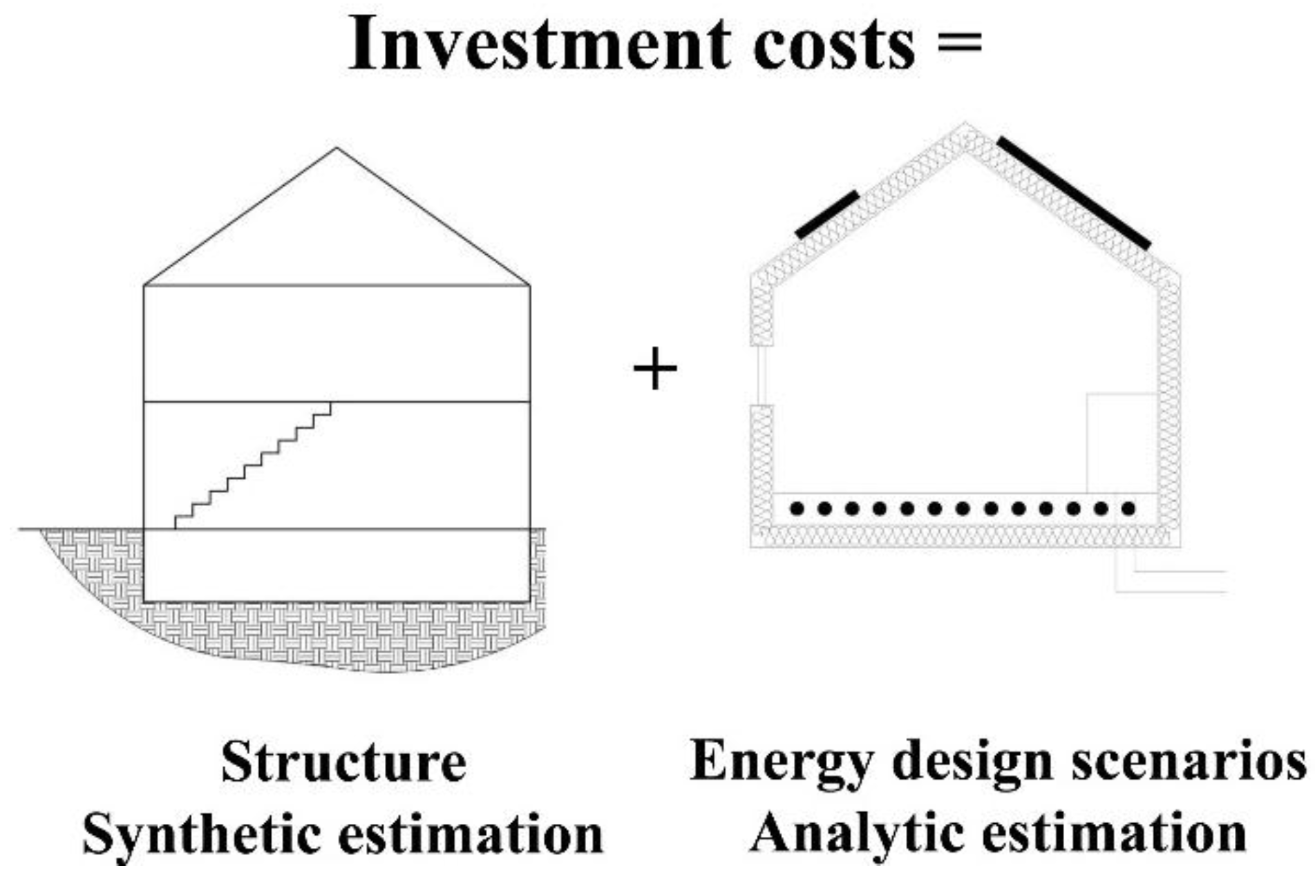
The main goal of this study was to test the cost-optimal analysis as a decision-making tool for supporting architects in the thermal design of nearly-zero energy buildings. This methodology was used to evaluate the energy performance and financial concerns during the whole building lifecycle for different design configurations; these included the building envelope and HVAC systems.
The analyzed basic example building consisted of a new three-story, 200-m2 single-family house located in Turin (Northern Italy), characterized by fairly cold winters and hot summers. Different design scenarios, with various envelope thermal insulation levels and HVAC system configurations, were defined. The aim of the study was to identify the most appropriate design scenario in terms of energy and economic performance, considering the basic design choices made by architects in terms of the performance features of some components of the project, such as envelope elements and systems. This means that it is possible to optimize the costs of the project and to reach at the same time an adequate energy performance by defining the design scenario with the lowest global cost. It is worth noting that in the present research, the evaluation of the costs is based on the consideration of the overall building and not only of the components related to the energy system, differently from the common applications of the global cost method. This choice can determine the contribution of the fixed costs of the building (i.e., without the costs related to the energy systems) on the final global cost.
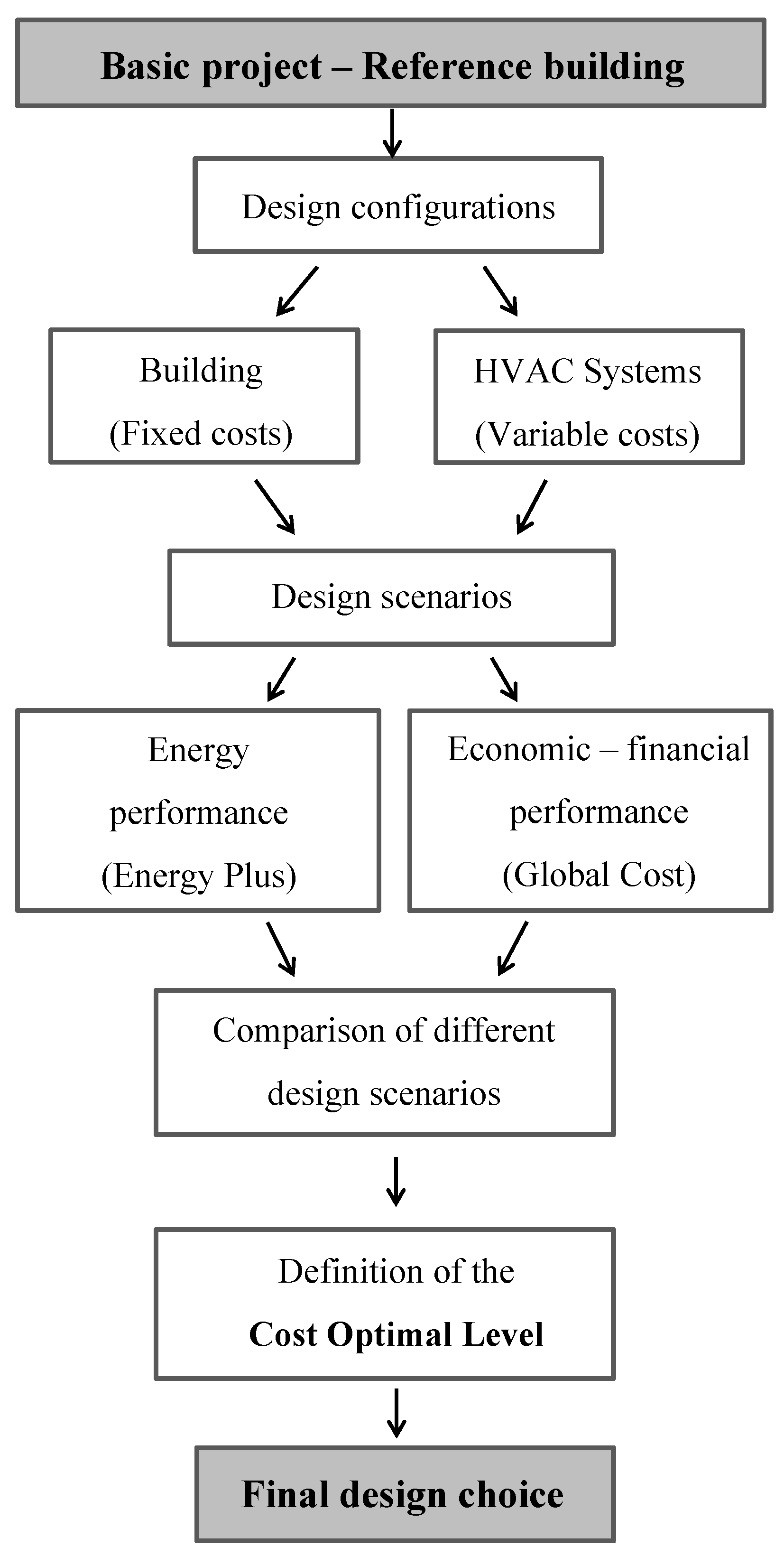
Figure 1 outlines how the cost-optimal methodology has been used for this study. As shown in the figure, the first step, after choosing the reference building (RB), was to identify design proposals for the building envelope and the HVAC systems. Furthermore, in order to align it with the requests for new nearly-zero energy buildings, these different design proposals were set to satisfy certain energy performance requirements. Combining the several design options in different design scenarios, it was possible to evaluate their energy and financial performance and to define the cost-optimal level in order to make a well-informed final design choice.
Figure 1.
Cost-optimal methodology applied to this study as a decision-making tool for supporting architects’ energy design choices.
Figure 1.
Cost-optimal methodology applied to this study as a decision-making tool for supporting architects’ energy design choices.
3. Cost-Optimal Methodology Background
Hereinafter, a description of the cost-optimal methodology is reported [
14,
15]. In particular, in this research, this methodology was tested as a decision-making tool to determine which design scenario represents the optimum in terms of energy and economic performance.
Cost-optimal methodology, as developed in this work, consists of different steps:
Step 1: Selection of the reference building that represents the basic design scenario [
16];
Step 2: Definition of some alternative design scenarios that provide for different solutions in terms of building envelope thermal insulation for four specific heat transfer levels and HVAC systems;
Step 3: Evaluation of the final and primary energy uses of the different design scenarios (including the reference building one);
Step 4: Economic evaluation of the hard costs due to construction;
Step 5: Economic evaluation of the operational costs due to energy consumption;
Step 6: Sensitivity analyses for the escalation of energy prices, variation of the calculation period and discount rate and the introduction of a tax credit.
3.2. Economic Performance Evaluation
The economic evaluation was carried out according to the procedure described in the European Standard EN 15459:2007 [
18], which provides a calculation method for the economic issues of heating systems and other systems that are involved in the energy demand and energy consumption of the building. This method can be used, fully or partly, for the following applications:
To consider the economic feasibility of energy saving options in buildings;
To compare different solutions of energy saving options in buildings (e.g., plant types, fuels);
To evaluate the economic performance of an overall design of the building (e.g., trade-off between the energy demand and energy efficiency of heating systems);
To assess the effect of possible energy conservation measures on an existing heating system, by the economic calculation of the cost of energy use with and without the energy conservation measure.
Particularly, the economic performance of the building is evaluated by means of the estimation of the global cost, which is calculated in Euros per square meter of gross floor area (€/m
2) and is directly linked to the duration of the calculation period τ. The global cost can be written as shown in Equation (1):
where
CG (
τ) represents the global cost referring to starting year
τ0,
CI is the initial investment cost,
Ca,i (
j) is the annual cost for component
j at year
i (including running costs and periodic or replacement costs),
Rd (
i) is the discount rate for year
i and
Vf,τ (
j) is the final value of component
j at the end of the calculation period (referring to the starting year
τ0). As shown in Equation (1), the total global cost is determined by summing up the global costs of initial investment costs, periodic and replacement costs, annual costs and energy costs and subtracting the global cost of the final value.
It is worth noting that Formula (1) makes use of the present value factor
fpv or the discount rate
Rd, which are used in order to match the costs to the starting year. Particularly, the discount rate coefficient
Rd is utilized for the replacement costs and the final value, while the present value factor
fpv is applied for the running costs that are equal for the overall period of the analysis. The formulas for the calculation of the discount rate and of the present value factor can be represented as follows:
where
RR is the real interest rate,
p is the year in which the replacement is made, while
n represents the number of years of the period under examination.
Replacement costs are calculated throughout the whole calculation period, while the final value of a specific system or envelope component is calculated from the remaining lifetime of the last replacement, assuming linear depreciation over its lifespan. In particular, the final value is determined as remaining lifetime divided by lifespan and multiplied by the last replacement cost and refers to the starting year with an appropriate discount rate.
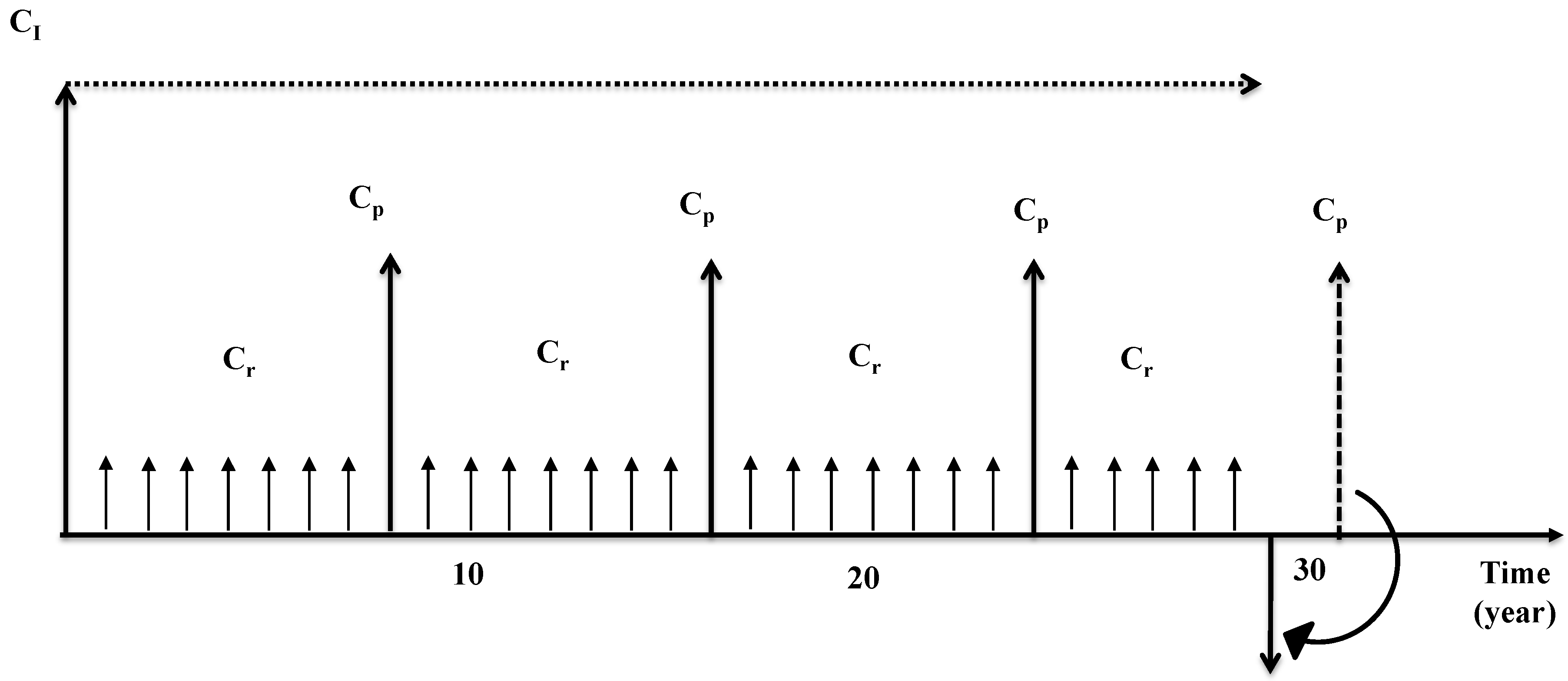
Figure 2 illustrates the concept of the final value given by EN 15459, where
CI is the initial investment cost to be considered when the building is delivered to the customer,
Cr are the running costs, which comprise maintenance costs, operational costs, energy costs and added costs, and
Cp are the replacement costs that are necessary due to the ageing of the various system and envelope components.
Figure 2.
Illustration of the final value concept.
Figure 2.
Illustration of the final value concept.
4. Application
In this study, four different design configurations were selected for both the building envelope and the HVAC system, in order to create various design scenarios, which can be evaluated by their energy and economic performances.
4.1. Design Configurations for Building Envelope
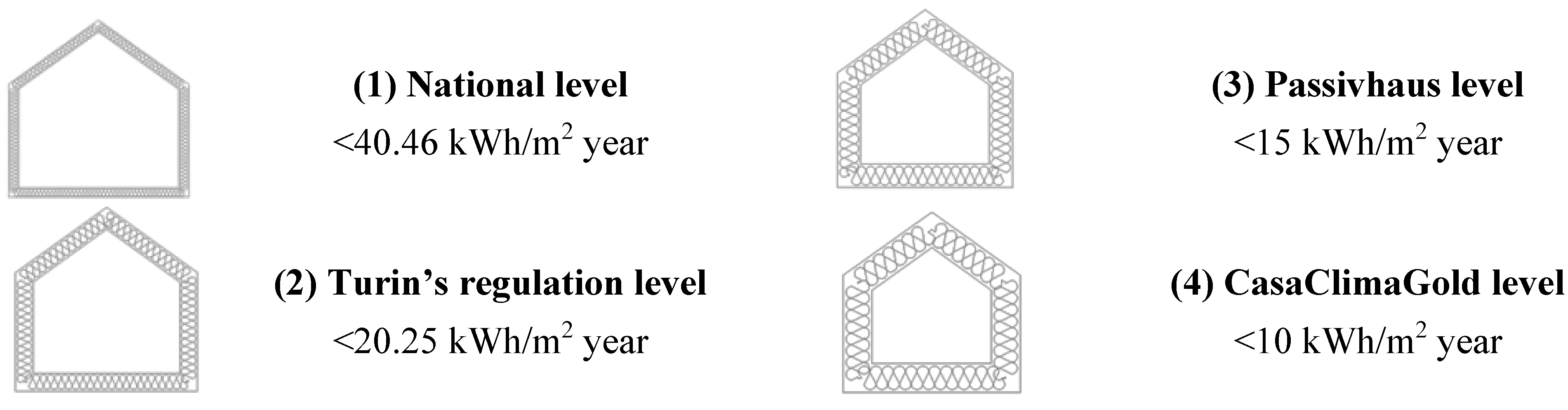
Four building envelope design configurations were chosen to fulfil different energy performance requirement levels for space heating, as illustrated in
Figure 3. The first level refers to the Italian directive for Climatic Zone E [
19] (where Turin is located); the second one refers to the optional value set by Turin’s regulations [
20]; the third one refers to the requirements necessary to obtain the classification of a Passivhaus [
21]; and the last one refers to the CasaClimaGold requirements [
22]. In particular, the national and Turin regulation requirements are expressed in terms of primary energy consumption for space heating, while the Passivhaus and CasaClimaGold ones represent the thermal energy need for space heating.
Figure 3.
Design levels for building envelope energy performances.
Figure 3.
Design levels for building envelope energy performances.
In order to satisfy these requirements, the building envelope was designed with four different thermal insulation degrees of the several building elements by varying the thickness of the insulation layer, the conductivity of the wall bricks and the thermal transmittance of the windows.
Every single building component (like walls and windows) had additionally to respect the thermal transmittance limits, fixed by each design level. Furthermore, using these particular design configurations for the building envelope, the energy efficiency classification improves (Classes A, A+), and so, the building market value is supposed to rise.
Table 1 summarizes the choices made for the different design configurations for the building envelope.
Table 1.
Design configurations for the building envelope.
Table 1.
Design configurations for the building envelope.
| Design levels | Component | U-value (W/m2K) | Insulation layer |
|---|
| National level (climatic zone E) | Walls | 0.26 | 8 cm |
| Roof | 0.21 | 15 cm |
| Ground slab | 0.26 | 10 cm |
| Windows | 1.8 | 4 + 15 + 4 mm (air) |
| Turin’s regulation level | Walls | 0.14 | 20 cm |
| Roof | 0.11 | 30 cm |
| Ground slab | 0.12 | 25 cm |
| Windows | 1.2 | 4 + 15 + 4 + 15 + 4 mm (air) |
| Passivhaus level | Walls | 0.09 | 25 cm |
| Roof | 0.09 | 35 cm |
| Ground slab | 0.10 | 30 cm |
| Windows | 0.8 | 4 + 15 + 4 + 15 + 4 mm (argon) |
| CasaClimaGold level | Walls | 0.07 | 35 cm |
| Roof | 0.07 | 45 cm |
| Ground slab | 0.08 | 40 cm |
| Windows | 0.7 | 4 + 12 + 4 + 12 + 4 mm (krypton) |
4.2. Design Configurations for Heating Ventilation and Air Conditioning Systems
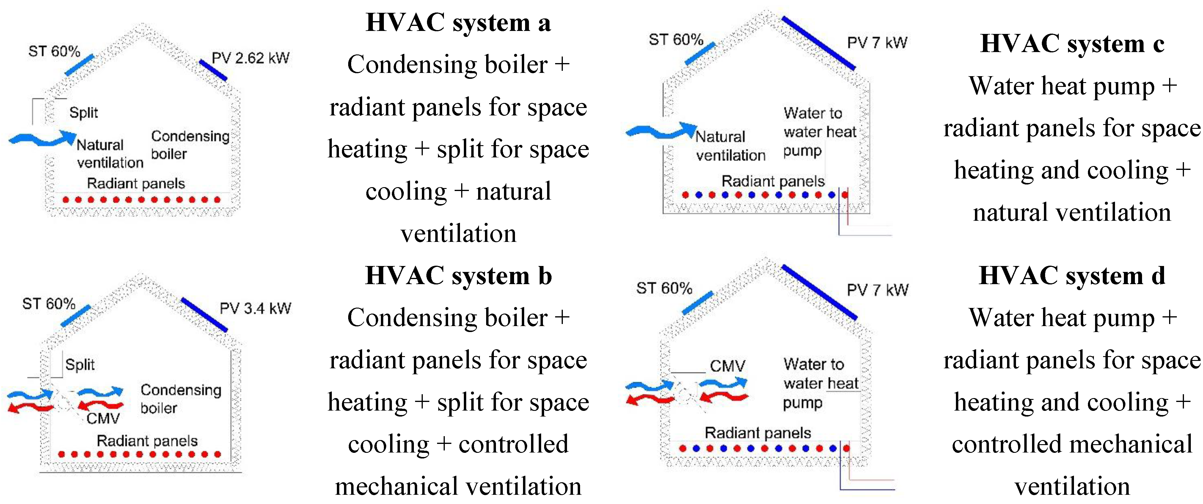
Furthermore, four different design configurations for the HVAC system were defined (
Figure 4). Indeed, in order to design a nearly-zero energy building, it is necessary to choose systems characterized by a high energy efficiency. The condensing boiler nominal efficiency was fixed equal to 0.95; the heat pump Coefficient of Performance for heating period (COP) was set equal to 4.75 and the Energy Efficiency Ratio (EER) for cooling period to 5.65.
Figure 4.
Design configurations for heating ventilation and air conditioning (HVAC) systems. ST: solar thermal panels, PV: photovoltaic panels, CMV: controlled mechanical ventilation.
Figure 4.
Design configurations for heating ventilation and air conditioning (HVAC) systems. ST: solar thermal panels, PV: photovoltaic panels, CMV: controlled mechanical ventilation.
According to the definition of a nearly-zero energy building, to reach the nearly-zero energy target, it is necessary to largely supply energy from renewable sources. Afterwards, in this study, some solar panels were installed, with a photovoltaic system, on the roof in order to cover 60% of the domestic hot water supply. The peak values of the PV panels refer to specific values from the Italian Directive [
23] in Systems 1 (2.6 kW
p) and 2 (3.4 kW
p), while the peak value of 7 kW
p in Systems 3 and 4 was defined in order to have a surplus of electricity production.
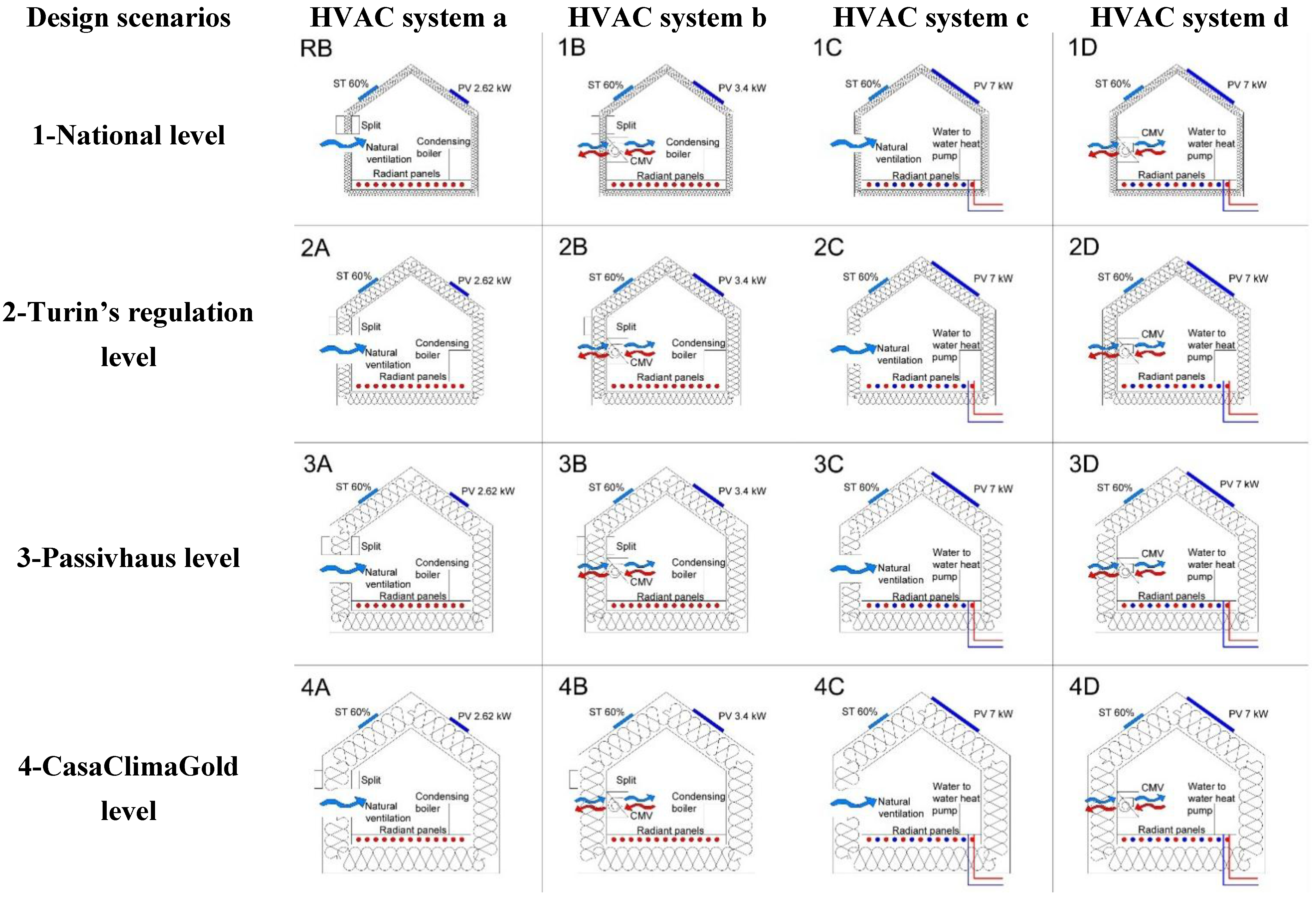
4.3. Design Scenarios
The last step was to combine the building envelope and the HVAC system design configurations in order to create different energy design scenarios that were evaluated in terms of energy and economic performance.
The recast of the Energy Performance of Buildings Directive [
7] recommends evaluating at least ten different design scenarios to make sure that enough design options are analyzed and the choice of one of this is well-informed. In this study, it was possible to create a 4 × 4 matrix, shown in
Figure 5, combining every building envelope design level with each of the four HVAC system configurations; consequently, there were 16 energy design scenarios to evaluate and compare. In
Figure 5, building envelope configurations are identified with a number, while different HVAC systems configurations are with a letter. The scenario 1a constitutes the basic scenario that represents the reference building, hereinafter called “RB-1a” in the following tables and graphs.
Figure 5.
Matrix of the 16 energy design scenarios.
Figure 5.
Matrix of the 16 energy design scenarios.
5. Energy Performance Evaluation
The goal of energy evaluation was to determine the annual energy consumption of the different design scenarios in terms of delivered energy, divided by sources, primary energy, divided by end uses (space heating and cooling, domestic hot water, mechanical ventilation, lighting and equipment), and the total.
The typical weather conditions of the Turin location are based on the Italian Climatic data collection Gianni De Giorgio (IGDG) Weather for Energy Calculation database of climatic data [
24].
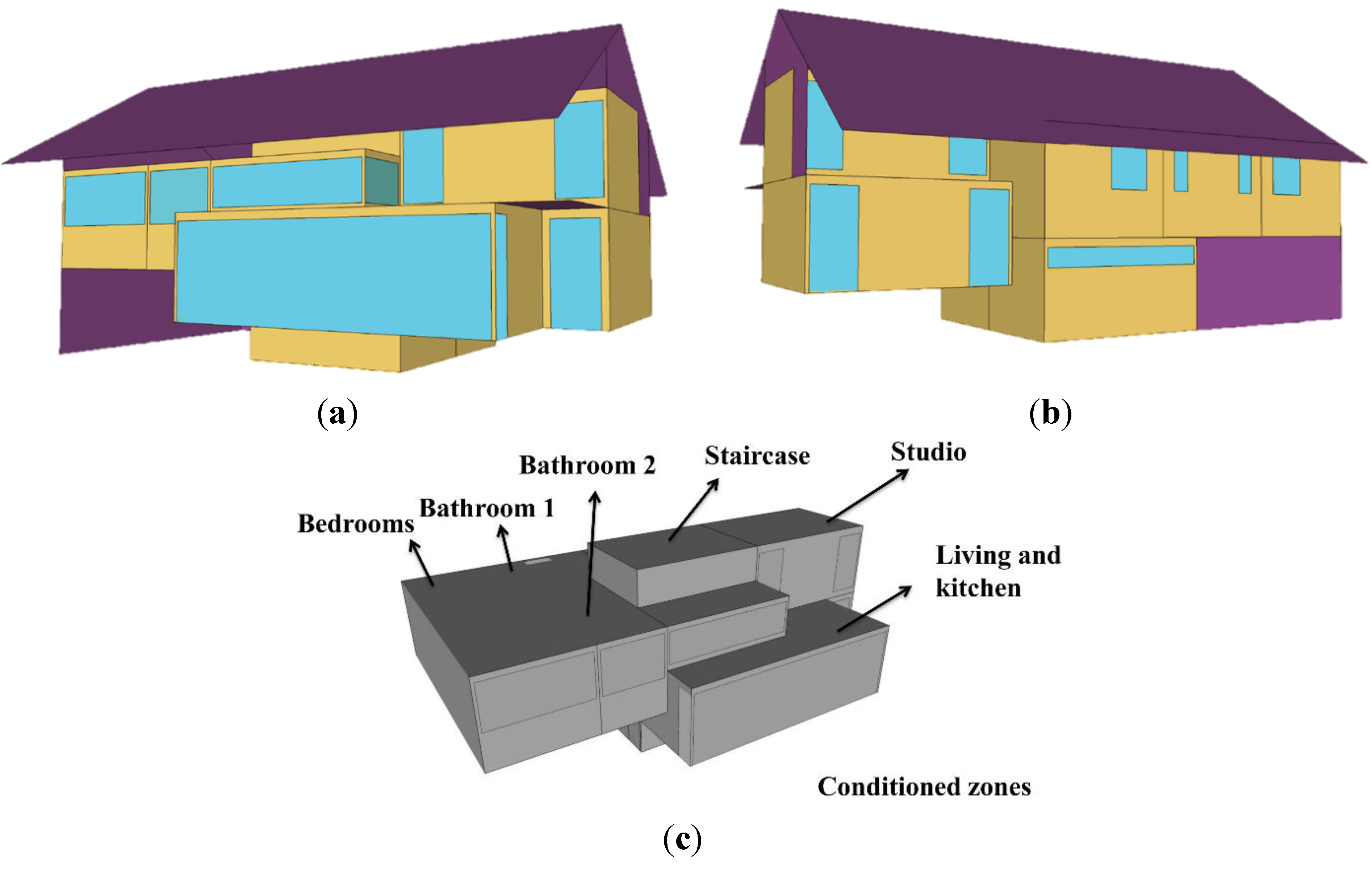
Figure 6 shows the geometric model of the three-story, 200-m
2 reference building [
16] and its division into six different conditioned thermal zones, for a better definition of the thermal loads. The net conditioned floor area is equal to 183 m
2.
Figure 6.
(a) Axonometric view: south façade; (b) Axonometric view: north façade; (c) Subdivision into thermal zones.
Figure 6.
(a) Axonometric view: south façade; (b) Axonometric view: north façade; (c) Subdivision into thermal zones.
The operational parameters were set to be consistent with the building typology. Particularly, for the occupancy level, the people per zone floor area were fixed to 0.04 person/m
2, according to Italian Standard UNI 10339 [
25]. Lighting and electric equipment maximum power densities were respectively defined equal to 4.5 W/m
2 and 2.98 W/m
2, according to European Standard ISO 13790 [
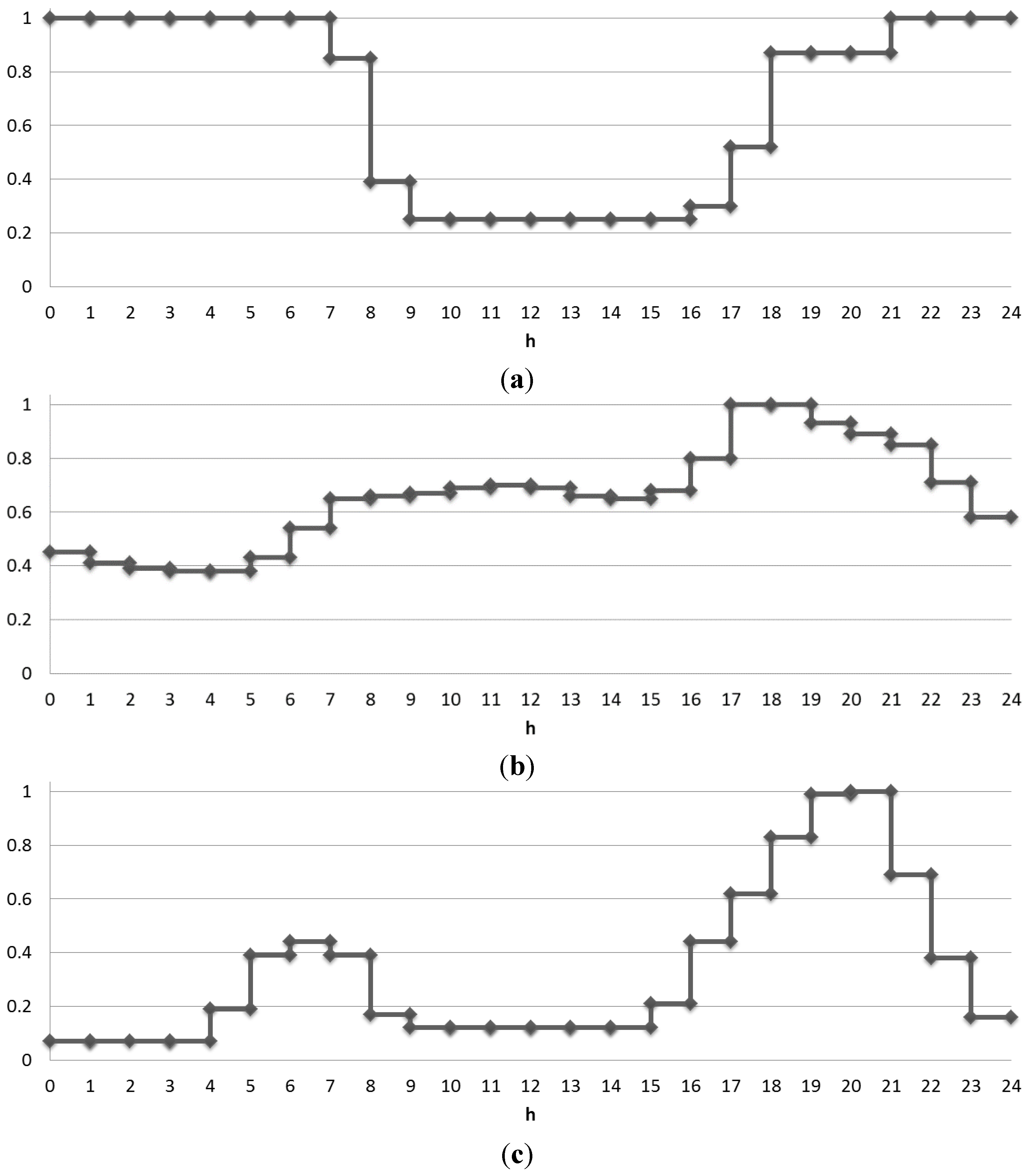
26]. Particularly, this standard defines the average internal heat gains values (which consist of the sum of heat gains due to people, lighting and equipment) for different building rooms on weekdays and weekends; the densities of people, lighting and equipment were set in order to respect these values. These densities were linked to the activity schedules carried out in the building during the weekdays and weekends and related to its use.
Figure 7 illustrates the schedules, which show temporal profiles during weekdays respectively for occupancy, lighting and equipment. These schedules refer to those of residential reference buildings available on the DOE dataset [
27].
Control of the solar shading was done on the basis of the total solar radiation incident on each window (above 300-W/m2 blinds, which are installed in the cavity between the glasses, are shut).
Scenarios A and C are naturally ventilated, while Scenarios B and D are characterized by the presence of a mechanical ventilation system. In all scenarios, the ventilation rate was set at 0.3 air change per hour (ach), while the infiltration rate was fixed equal to 0.1 ach.
The heating system was assumed to be active from the 15 October to 15 April, according to Italian regulations for Climatic Zone E (Turin). The cooling system was set to operate from the 30 April to 30 September. During all days, the heating set point was fixed to 20 °C from 7 a.m. to 8 p.m. and to 18 °C during the rest of the day, while the cooling set point was established as equal to 26 °C from 7 a.m. to 5 p.m. and to 28 °C during the other hours of the day.
Figure 7.
(a) Occupancy schedule; (b) Equipment schedule; (c) Lighting schedule.
Figure 7.
(a) Occupancy schedule; (b) Equipment schedule; (c) Lighting schedule.
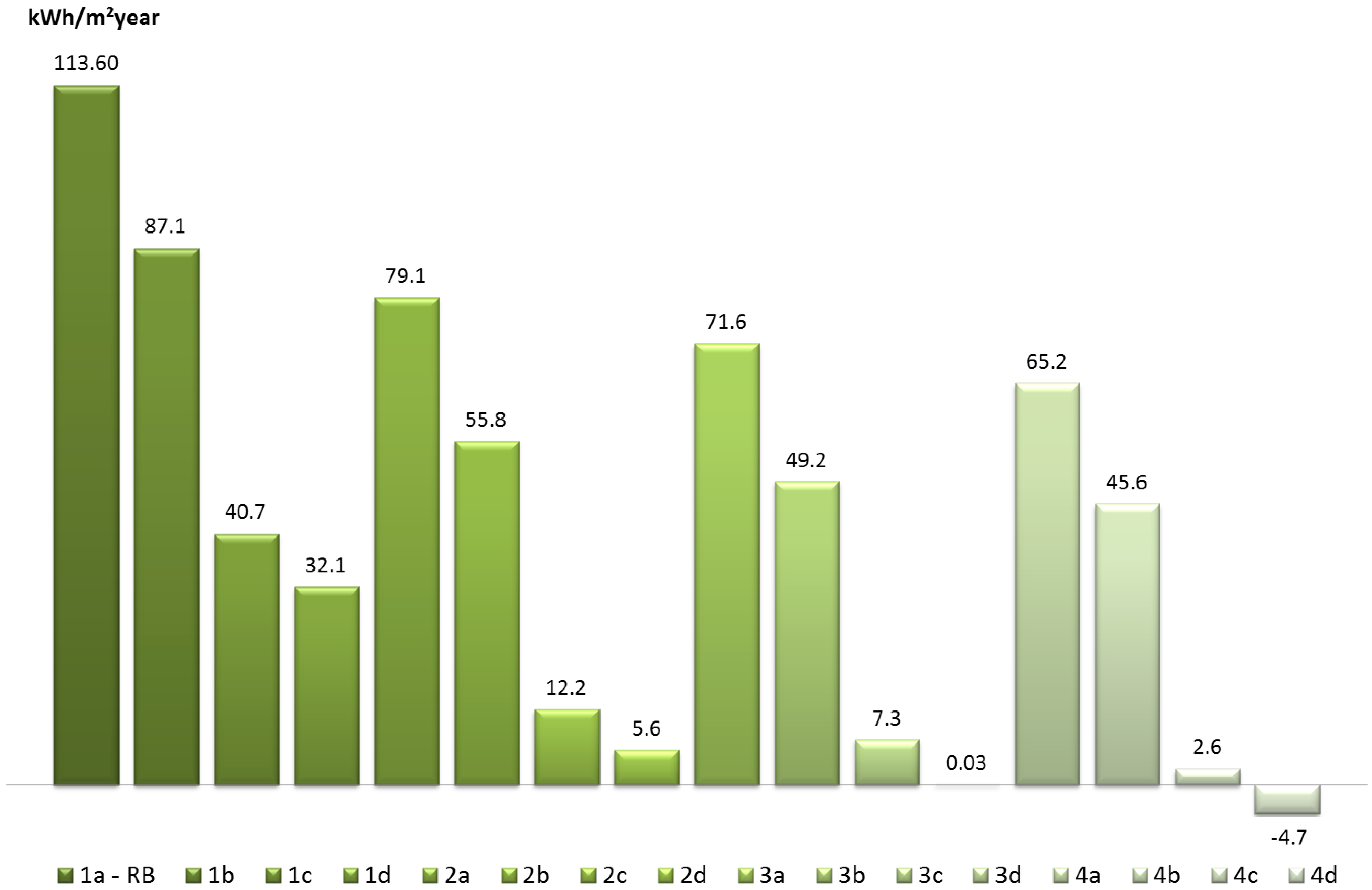
Figure 8 summarizes primary energy consumptions for every analyzed design scenario; annual primary energy consumption includes the energy for space heating and cooling, ventilation, lighting, equipment and domestic hot water. The amount of primary energy produced by the renewable energy sources (solar and photovoltaic panels installed on the roof) has been subtracted form total consumption in order to consider the net building primary energy delivered. Indeed, according to the cost-optimal methodology that expresses all energy uses with a single primary energy indicator, the renewable sources-based technologies enter into direct competition with the demand-side solution; this is in line with the purpose of the cost-optimal calculation to identify the solution that represents the least global cost without discriminating against or favoring a certain technology.
As shown in
Figure 8, some scenarios reach the nearly-zero energy goal, and the last one (4d) even reaches the plus-energy target, which means that this energy design configuration produces more energy than necessary for the building demand.
Figure 8.
Primary energy consumption for every energy design scenario.
Figure 8.
Primary energy consumption for every energy design scenario.
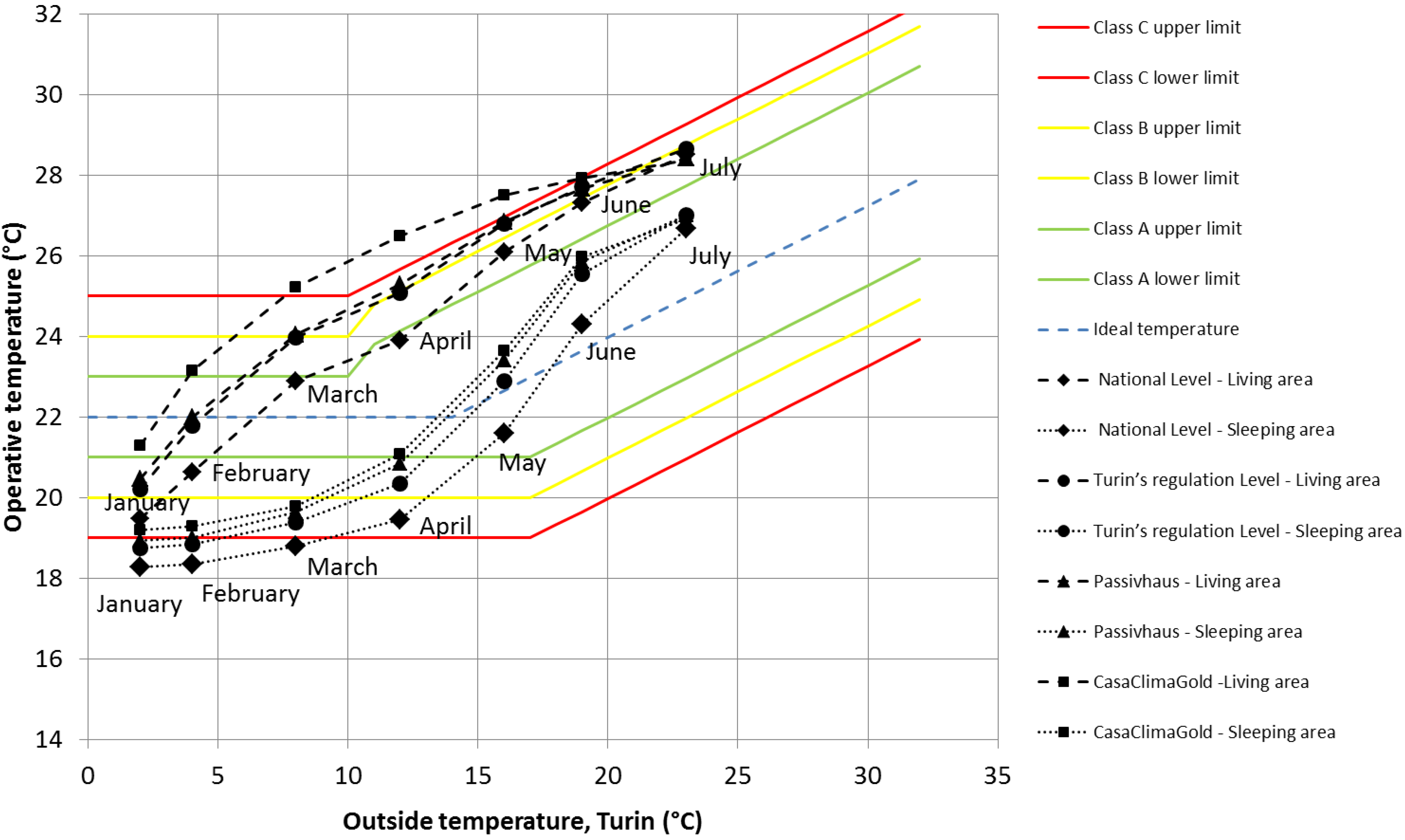
Thermal Indoor Environment Assessment
A critical aspect in designing an nearly-zero energy buildings (nZEB) is that the energy demand reduction by increasing indiscriminately the thermal insulation thickness delivers a drop in the indoor thermal comfort, especially in a Mediterranean climate (Turin). Indeed, this kind of superinsulation can lead to important problems during the summer period due to overheating of the indoor building environment [
28]. Furthermore, the cost-optimal methodology does not take into account in any way the indoor comfort conditions.
Some envelope design configurations analyzed in this study consider insulation layers up to 45 cm (such as CasaClimaGold). Therefore, in order to keep the overheating phenomenon related to increasing the thermal insulation in different design scenarios under control, it was necessary to examine the variation of indoor temperature. In the investigation performed of the indoor environmental quality, only the operating temperature was analyzed. Relative humidity was not considered in this analysis, even if it can be a significant factor; nevertheless, relative humidity control is not typically carried out in the residential Italian market.
In detail, for every design scenario and for the living and the sleeping area of the building, the medium monthly indoor operating temperature was estimated; only the performance of the building envelope was taken into account, without considering the presence of an HVAC system. The indoor operating temperature (separated for the two building areas) was plotted
versus the monthly outdoor temperature of Turin in a graph in which thermal comfort classes are reported according to EN 15251 [
29] (
Figure 9); the blue dashed line represents the optimal monthly operating temperature at which the indoor environment has to be maintained according to EN 15251, referring to the adaptive comfort theory. Observing the graph, it seems appropriate to choose design configurations that include either the provincial level or the Passivhaus level requirements in terms of envelope thermal transmittance. The scenario that corresponds to the national level of thermal insulation is not appropriate in the winter period, since there is too little of an insulation layer to ensure an indoor operating temperature that is over the lower limit of thermal comfort Class C (especially for the sleeping area, which coincides with the lowest curve). On the other hand, the scenario that has a thermal insulation level typical of a CasaClimaGold is not suitable during the summer period, since a too high of an insulation layer leads to high temperatures in the indoor environment (especially in the living area, the highest curve), superior to the upper limit of thermal comfort Class C.
Figure 9.
Comparison between different envelope levels of thermal insulation related to design scenarios in terms of monthly indoor operating temperature. Data from EN 15251:2008 [
29].
Figure 9.
Comparison between different envelope levels of thermal insulation related to design scenarios in terms of monthly indoor operating temperature. Data from EN 15251:2008 [
29].
7. The Cost-Optimal Level
After evaluating primary energy consumptions and global costs for every design scenario, it is possible to draw the graph of the cost-optimal and the related cost curve, the minimum of which represents the cost-optimal level. The following paragraphs outline the numerical results of the global cost calculation and the subsequent steps of the cost-optimal analysis.
7.1. Numerical Results
The final results of the global cost calculation for every energy design scenario are summarized in
Table 3. The global costs of the several design scenarios unveil a cost range over 30 years between 2008 and 2355 €/m
2. The reference building is characterized by the highest global cost, since the energy costs are more significant than in the other scenarios.
Table 3.
Numerical results for the global cost calculation over 30 years. RB: reference building.
Table 3.
Numerical results for the global cost calculation over 30 years. RB: reference building.
| Energy design scenario | Investment cost (€/m2) | Annual energy costs (€/m2year) | Annual maintenance costs (€/m2year) | Final value (€/m2) | Replacement costs (€/m2) | Global cost (€/m2) |
|---|
| 1a-RB | 1724 | 40 | 2.5 | 289 | 83 | 2354 |
| 1b | 1789 | 31 | 4.7 | 316 | 115 | 2288 |
| 1c | 1882 | 12 | 4.6 | 366 | 158 | 2008 |
| 1d | 1913 | 10 | 6.4 | 375 | 175 | 2039 |
| 2a | 1759 | 23 | 2.5 | 293 | 83 | 2051 |
| 2b | 1823 | 17 | 4.7 | 319 | 115 | 2040 |
| 2c | 1917 | 8 | 4.6 | 369 | 158 | 1947 |
| 2d | 1948 | 7 | 6.4 | 378 | 175 | 2007 |
| 3a | 1857 | 19 | 2.5 | 295 | 83 | 2067 |
| 3b | 1924 | 11 | 4.7 | 322 | 115 | 2034 |
| 3c | 2018 | 7 | 4.6 | 372 | 158 | 2039 |
| 3d | 2049 | 7 | 6.4 | 381 | 175 | 2097 |
| 4a | 1894 | 15 | 2.5 | 299 | 83 | 2026 |
| 4b | 1958 | 9 | 4.7 | 326 | 115 | 2020 |
| 4c | 2051 | 6 | 4.6 | 376 | 158 | 2048 |
| 4d | 2082 | 6 | 6.4 | 385 | 175 | 2112 |
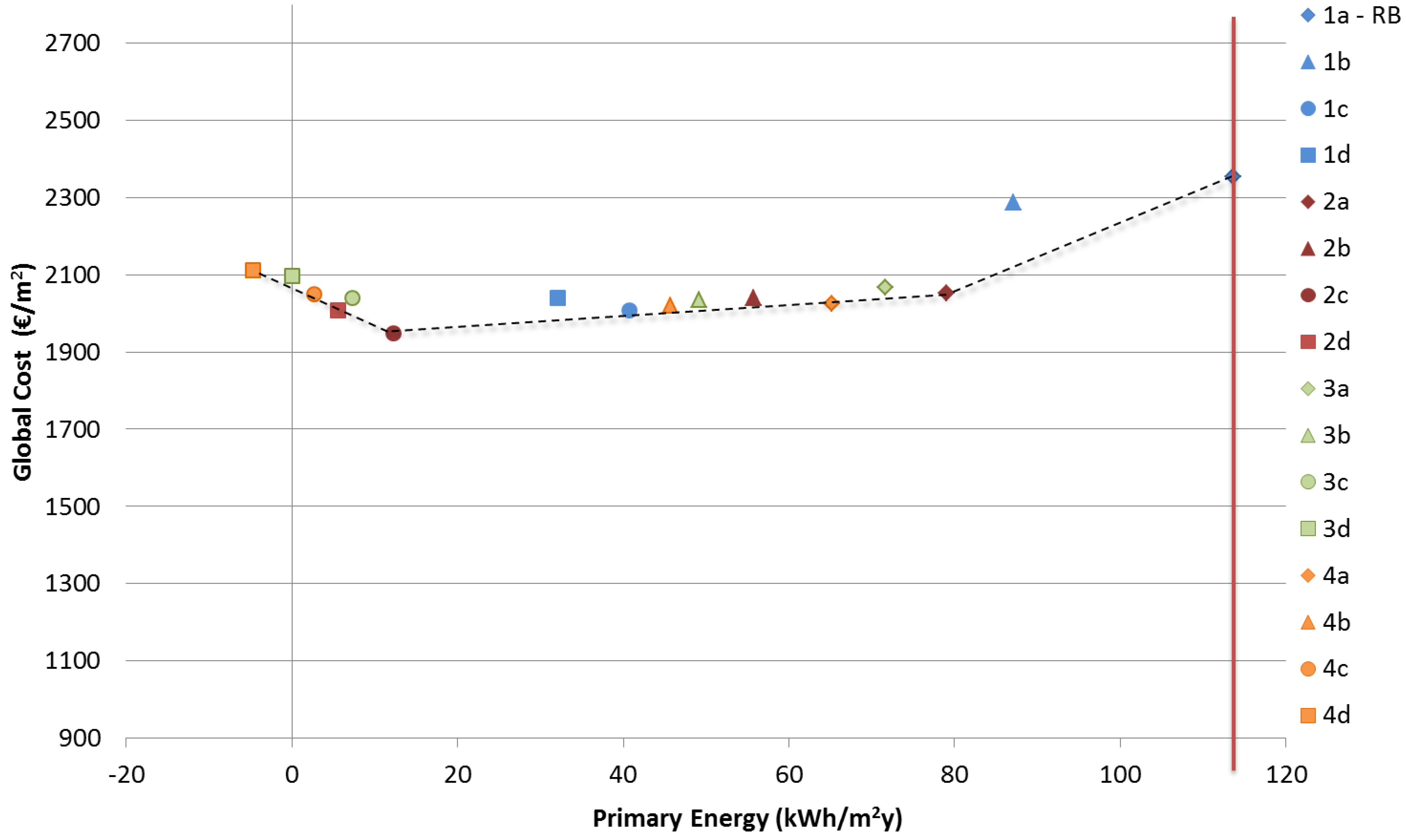
7.2. Cost-Optimal Curve
In order to find the cost-optimal level, the primary energy consumption on the
x-axis (kWh/m
2·year) has been plotted
versus the global cost (
Figure 11) on the
y-axis (€/m
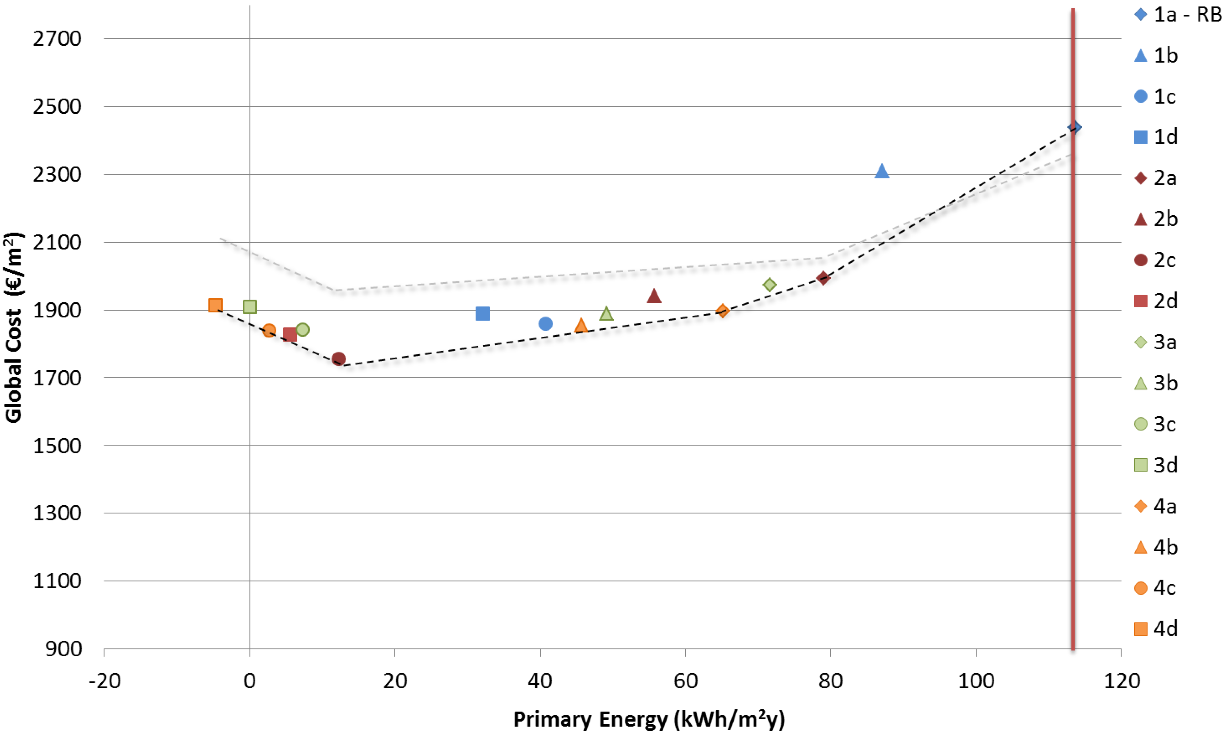
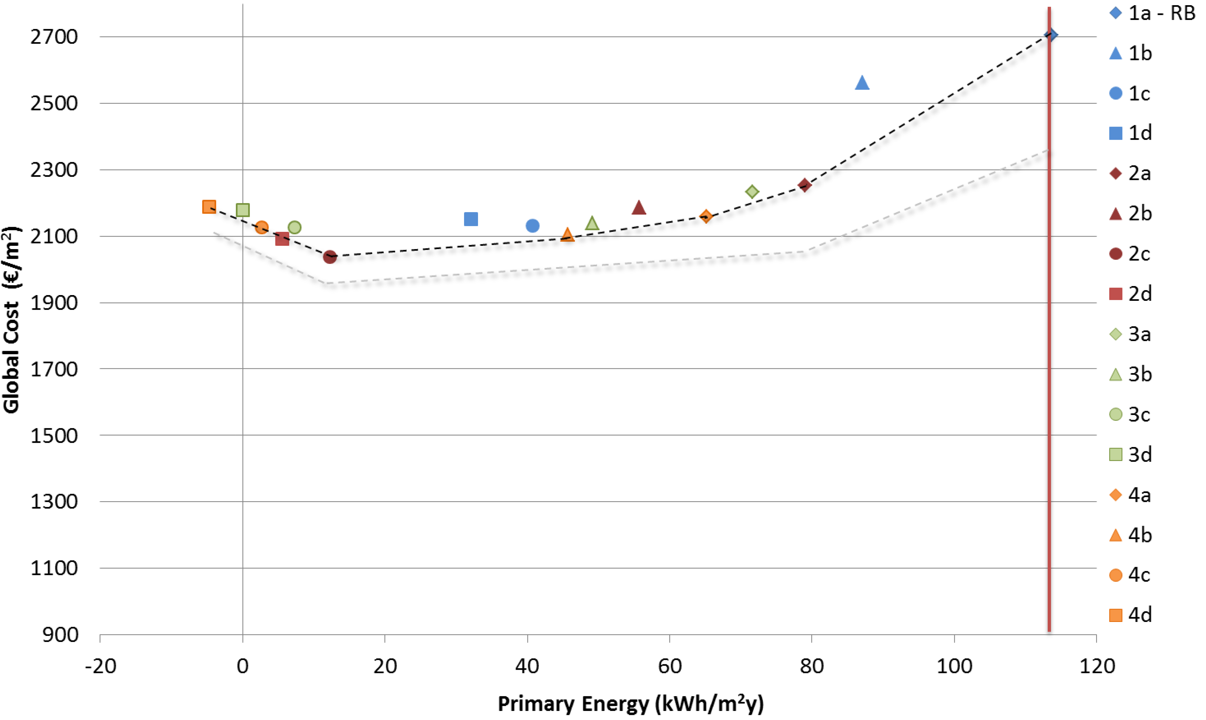
2). In the graph, in correspondence with the reference building, which represents the basic design scenario (1a-reference building (RB)), a red vertical line, which represents the maximum primary energy consumption, was drawn; the reference scenario is the least energy and economic performing scenario.
Each point on the graph represents a different design scenario in terms of energy and economic performance. The positions of the different scenarios permitted drawing the trend of the dotted broken line that represents the cost curve, the minimum of which may be considered as the cost-optimal level.
Analyzing the graph in terms of primary energy consumptions, several design scenarios fulfil the nearly-zero energy building target (2c, 2d, 3c, 3d, 4c) and even one amounts to a positive-energy scenario (4d). All of those scenarios are characterized by the presence of radiant panels (both for space heating and cooling) with the water heat pump associated with natural (c) or mechanical ventilation (d). It is worth noting that all of them have installed the photovoltaic system with the uppermost pick power; this demonstrates that the contribution of renewable sources for reaching the nZEB target is fundamental.
The cost-optimal level consists of design Scenario 2c (Turin’s regulation thermal insulation level, water heat pump, radiant panels for space heating and cooling, natural ventilation). Since their global costs values are close together, it is possible to say that Scenarios 2d (Turin’s regulation thermal insulation level, water heat pump, radiant panels for space heating and cooling, mechanical ventilation) and 1c (the national thermal insulation level, water heat pump, radiant panels for space heating and cooling, natural ventilation) are in the so-called cost-optimal range. Nevertheless, Scenario 1c does not represent an nZEB. Indeed, Scenarios 2d and 1c require the same amount of global cost, but the first one presents a total primary energy consumption of only about 5 kWh/m2·year, while this value increases for Scenario 1c to 40 kWh/m2·year. This is the evidence that similar global cost values lead to buildings with different energy performance, up to reaching a nearly-zero energy building.
Figure 11.
Cost-optimal graph.
Figure 11.
Cost-optimal graph.
8. Sensitivity Analyses
The European Guidelines [
15] outline that Member States should at least perform three different kinds of sensitivity analyses in order to test the stability of the results obtained by the global cost calculation. Sensitivity analysis concerns a “what if” kind of questions to see if the final answer is stable when the inputs are changed. Sensitivity analysis is standard practice in
ex ante assessments when outcomes depend on the assumptions of key parameters, of which the future development can have a significant impact on the final result.
For this study, four types of sensitivity analyses were carried out:
Escalation of energy prices with an annual percentage rate of 2.8%;
Reduction of the calculation period (20 and 10 years);
Variation of the discount rate (5%, 1% and 0.5%);
Introduction of tax credits, referring to the investment cost, with a percentage rate of 65% and 36%.
8.1. Escalation of Energy Prices
This analysis considered an escalation of energy prices with an annual percentage rate of 2.8% [
33], while the original global cost calculation took into account constant prices during the whole calculation period (light grey curve).
As shown in
Figure 12, scenarios with low primary energy consumption are less sensible in this kind of analysis, and the global cost varies only about 50 €/m
2; design scenarios with the lowest energy performance, and particularly the reference building, vary their global cost up to 300 €/m
2. This is why, after this first sensitivity analysis, the final design choice should consider the scenarios that consume less than 20 kWh/m
2·year of primary energy; the cost-optimal level is always represented by energy design Scenario 2c (Turin’s regulation thermal insulation level, water heat pump, radiant panels for space heating and cooling, natural ventilation).
Figure 12.
Sensitivity analysis with regard to the escalation of energy prices.
Figure 12.
Sensitivity analysis with regard to the escalation of energy prices.
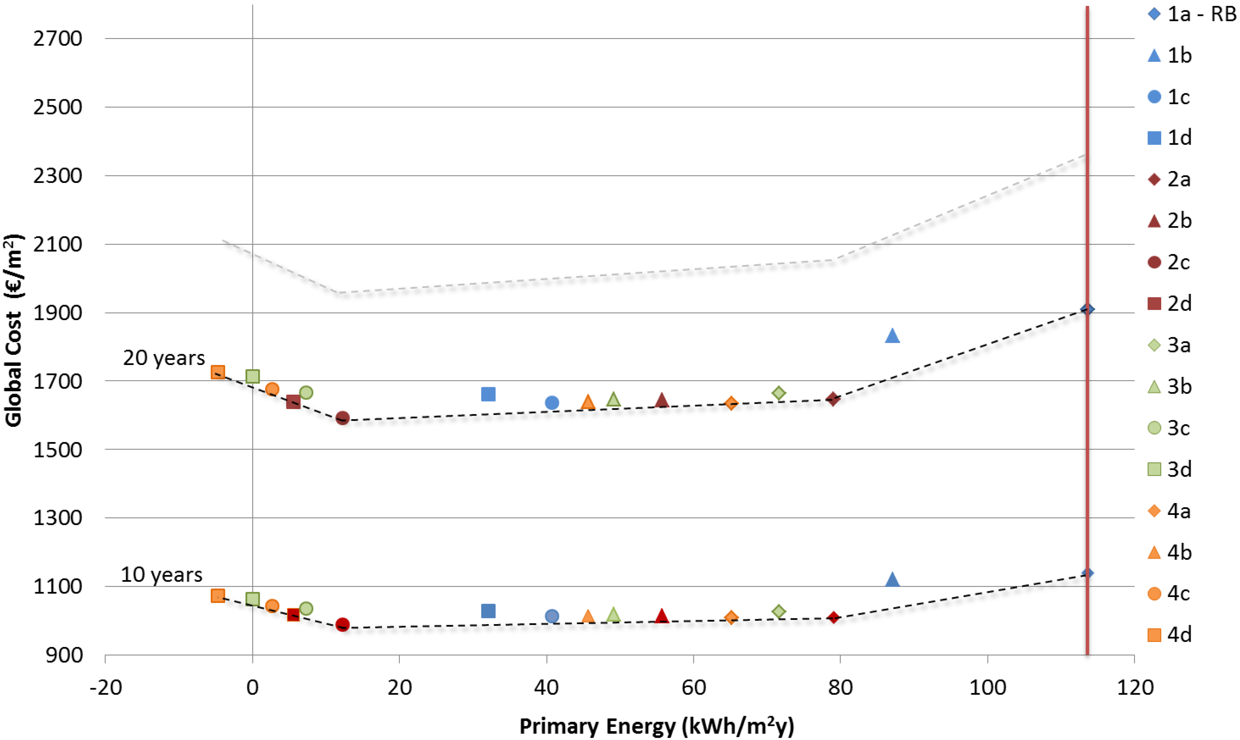
8.2. Reduction of the Calculation Period
Furthermore, the sensitivity analysis is relevant with reference to the reduction of the calculation period. The basic analysis took into account 30 years, which is the period indicated by the regulation [
14] for residential buildings. In this sensitivity analysis, this period was shortened up to 20 and 10 years in order to evaluate the contingent financial return for investors.
Figure 13 shows that the reduction of the global cost compared to the original analysis (light grey curve) is quite significant; this is due to the fact that few building components had to be replaced throughout the calculation period and their final value raised. In this analysis, the cost-optimal level still does not change and is still made up by energy design Scenario 2c (Turin’s regulation thermal insulation level, water heat pump, radiant panels for space heating and cooling, natural ventilation).
Figure 13.
Sensitivity analysis with regard tothe reduction of the calculation period to 20 and 10 years.
Figure 13.
Sensitivity analysis with regard tothe reduction of the calculation period to 20 and 10 years.
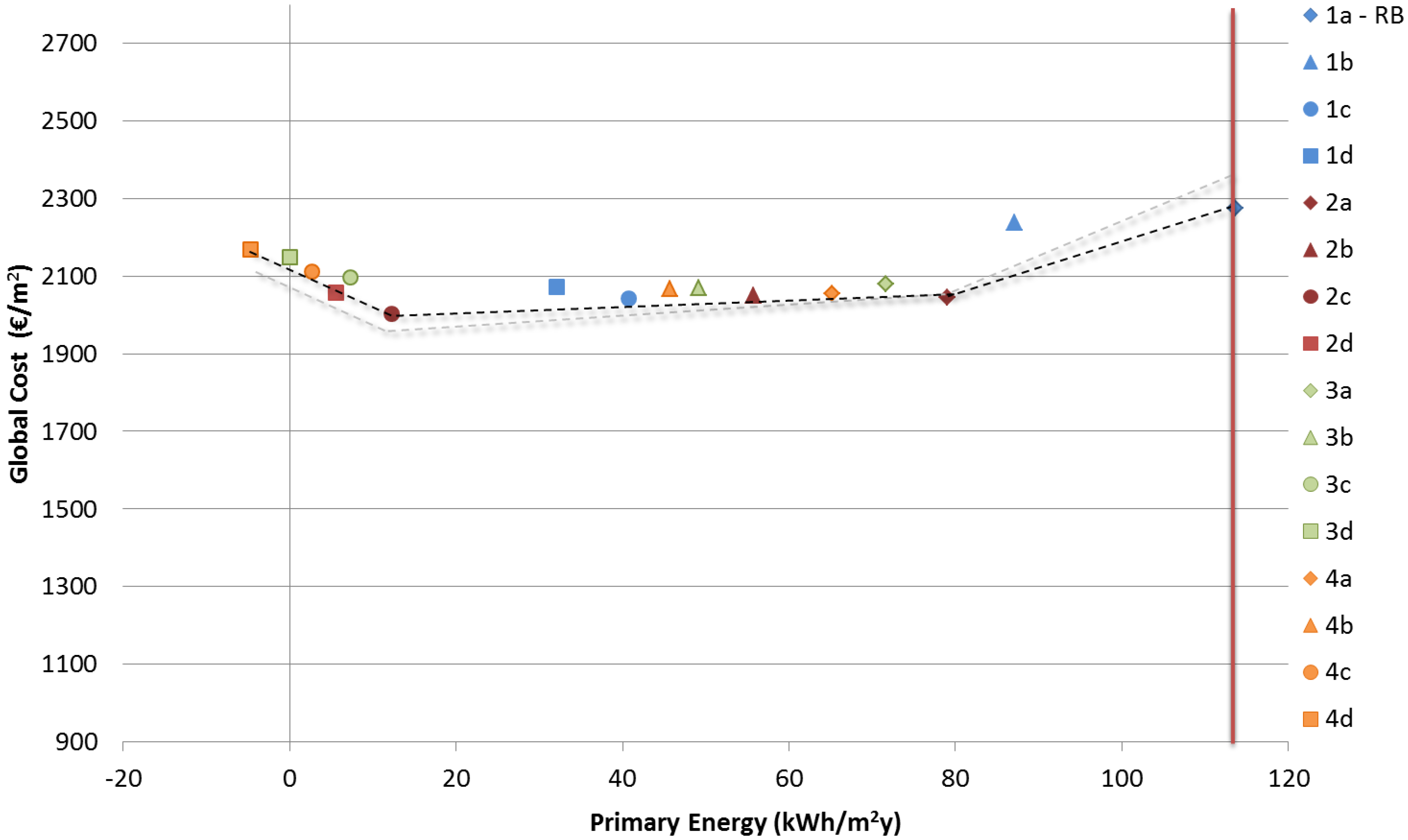
8.3. Variation of the Discount Rate
This sensitivity analysis took into account the variation of the discount rate, which amounted to 5% in the first case and to 0.5% in the second one, in order to adopt a financial and economic evaluation. The basic analysis (light grey curve) considered a discount rate of 3%. Furthermore, in this kind of analysis, the cost-optimal level remained the same, 2c (Turin’s regulation thermal insulation level, water heat pump, radiant panels for space heating and cooling, natural ventilation).
In the first hypothesis (discount rate = 5%), shown in
Figure 14, the global cost of the best energy performing design scenario raised, while in the second hypothesis (discount rate = 0.5%), shown in
Figure 15, this value significantly dropped. This is due to the fact that the final value incidence in these design scenarios is more significant than that of the running costs. In both sensitivity analyses, the cost-optimal level is still represented by design Scenario 2c.
Figure 14.
Sensitivity analysis with regard to the variation of the discount rate to 5%.
Figure 14.
Sensitivity analysis with regard to the variation of the discount rate to 5%.
Figure 15.
Sensitivity analysis with regard to the variation of the discount rate to 0.5%.
Figure 15.
Sensitivity analysis with regard to the variation of the discount rate to 0.5%.
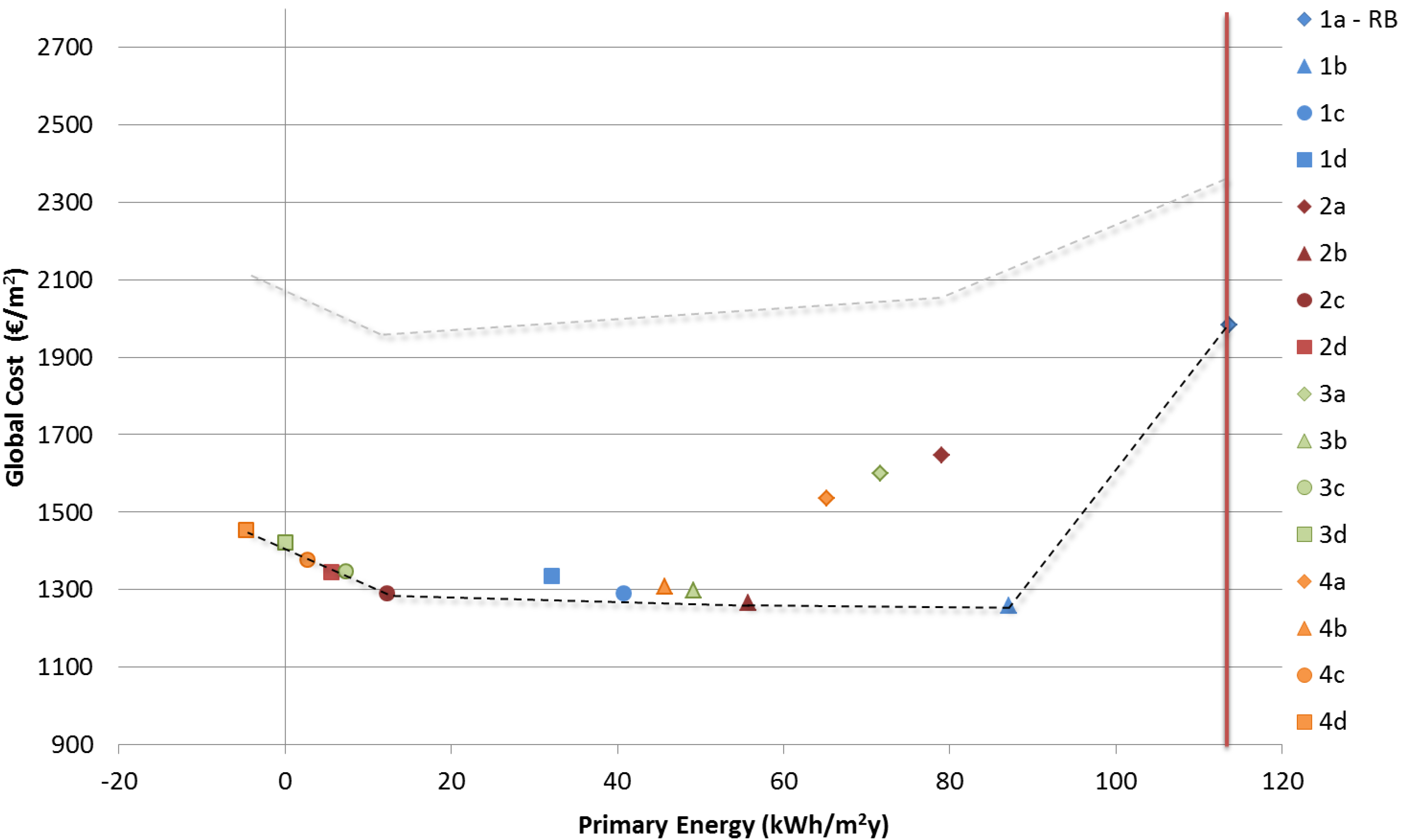
8.4. Introduction of Tax Credits
The last sensitivity analysis considered the Italian financial subsidy concerning buildings [
34]; indeed, it is possible to be awarded a tax credit amounting to 65%.
In
Figure 16 is shown the variation of the cost curve referring to a tax credit amounting to 65%. The global cost of all design scenarios reduced significantly. It seems really interesting that design scenarios with low energy performance (1b, 2b, 3b, 4b, 1c) have now lower global cost value than those of high performing scenarios. This is due to the fact that high energy performing scenarios require high initial investment costs, while the access to the tax credit is characterized by spending limits of 100.000 €. Since the global cost value of Scenario 2c, which represented the optimum in all other previous analyses, lied close to those of the low energy performing scenario mentioned above, it is possible to declare that also this sensitivity analysis confirmed the results.
Figure 16.
Sensitivity analysis with regard to tax credits in the amount of 65% of the initial investment costs.
Figure 16.
Sensitivity analysis with regard to tax credits in the amount of 65% of the initial investment costs.
9. Conclusions
The main goal of this study was to show how the cost-optimal methodology can be exploited as a decision-making tool by architects in order to evaluate and compare the energy and economic performance of different design scenarios. In particular, in this research, the cost-optimal methodology was applied to a new single-family house located in the North of Italy, which was designed to be a nearly-zero energy building. This method was chosen to define how energy and economic aspects could influence the preliminary design phase of the project and, in particular, the choice of the performance features of some components, such as envelope elements and systems. Therefore, different design scenarios, with various envelope thermal insulation levels and HVAC system configurations, were defined. The aim of the study was to identify the cost-optimal level that represents the most appropriate design scenario in terms of energy and economic performances. The stability of the results was also tested by carrying out some sensitivity analyses.
This study shows that investing in nearly-zero energy design scenarios is advantageous, not only in terms of energy performance, but also for economic issues. Spending the same amount of money during the whole building lifecycle in terms of global cost value, it is possible to design buildings that have a reduced impact on the environment thanks to their high energy saving, and at the same time, they are economically viable. The higher initial investment costs are compensated by the low energy consumptions, which permit one not only to save energy and, consequently, to reduce CO2 emissions, but also to drop the investment of economic resources.
The results of the different analyses carried out during this research demonstrate that the most viable design scenario (2c) is related to Turin’s city regulation level of envelope thermal insulation and to an HVAC system that consists of a water heat pump, radiant panels for space heating and cooling, natural ventilation and in which a large amount of energy is supplied form renewable sources. This demonstrates that the contribution of renewable sources for reaching nZEB targets is fundamental. However, it should be stressed that all of the analyzed zero-energy design scenarios differ from the cost-optimal value by a maximum of 150 €/m2, which represents a reasonable amount.
It is possible to make some considerations about the applied methodology itself. Even if the cost-optimal analysis can be considered an efficient tool for the evaluation of the energy and economic performances of the building and valid help for the choice between several design configurations, it is necessary to outline that this methodology represents a rather complex procedure in the preliminary phase of project planning. The methodology itself requires a large number of detailed input data, which often are not yet defined in the preliminary phase of the project, which constitutes a crucial moment for architects’ design decisions. Furthermore, even if cost-optimality as a theoretical concept is well and clearly established, its application is far from easy and straightforward and needs quite a long time to be applied. This is in contrast with the inherent necessity of the preliminary phase to have an assessment tool that allows the testing of a large number of energy design configurations in a short time.
Furthermore, the methodology is not complete, and architects have to carry out studies with the cost-optimal analysis to assure a complete and successful energy building design. For instance, it does not take into account in anyway the evaluation of the indoor comfort quality, which needs to be assessed in parallel.
Moreover, a very promising line of research is constituted by the integration of the cost-optimal methodology with other methods used for the estimation of the market value of properties, such as, for example, the hedonic pricing method. Given a certain market segment, the application of the hedonic pricing method would permit the evaluation of the willingness-to-pay of the users for an improvement in the energy efficiency of the house. The value of the WTP could be compared with the value of the global cost of the improvement in order to understand if any extra value exists. In other words, the integration of the aforementioned approaches could clarify if improvements in energy efficiency can lead to an increase in the market value of housing assets. At this moment, little research has been published on this subject [
35].
Finally, in this study, sixteen design scenarios have been evaluated and compared in terms of energy performance and economic issues, but further studies could be made by simulating other different envelope and system technological configurations and performing other types of sensitivity analyses. For instance, another interesting sensitivity analysis could concern the variation and implementation of the initial investment costs and replacement costs. It could be interesting also to explore the use of different discount factors (e.g., hyperbolic discounting) for the calculation of the present values to be included in the evaluation model [
36]. Moreover, the global cost formula utilized in this research does not consider the CO
2 emissions and the disposal costs at the end of the lifecycle and has still to be experimented upon in the interest of a complete energy and economic evaluation. Finally, the maintenance costs have been calculated only for the HVAC systems, while it would be useful to outline these types of costs also for the building envelope components (which in this specific study have not been calculated). It seems clear that an increase of analyses will lead to more reliable final design choices.


 and
and 


