
Aeolian Vibration Dynamic Analysis of Large-Span, Relaxed Antenna Cable Net Based on Finite Particle Method

1
Space Structure Research Center, Zhejiang University, Hangzhou 310030, China
2
Beijing Institute of Architectural Design, Beijing 100055, China
3
Naval Research Institute, Beijing 100161, China
*
Authors to whom correspondence should be addressed.
Buildings 2024, 14(1), 105; https://doi.org/10.3390/buildings14010105
Submission received: 10 November 2023
/
Revised: 13 December 2023
/
Accepted: 21 December 2023
/
Published: 30 December 2023
(This article belongs to the Special Issue Advancements in Large-Span Steel Structures and Architectural Design)
Abstract
:The large-span, relaxed antenna network is a large deformation flexible structure due to its low pre-tension level of the wires. Its dynamic analysis under a wind load belongs to dynamic and geometric nonlinear problems, which is very complex to accurately calculate and solve. This paper explores the possibility of the finite particle method (FPM) to the aeolian vibration analysis of a large-span, low stress-tensioned antenna cable net. In the FPM, the antenna network structure is discretized into a group of finite particles, where the motions of all particles follow Newton’s second law and can be solved dynamically using a central difference scheme. The effectiveness and applicability of the FPM were verified by comparing the calculation results of the finite element method and FPM. The FPM was used to study the effects of wind speed and the distribution of vibration on the aeolian vibration of antenna cable nets. The results showed that this method is suitable for studying the aeolian vibration of a large-span, low stress-tensioned antenna network and has high computational efficiency and accuracy.
1. Introduction
The long wave antenna mainly uses very low frequency (VLF) technology to serve the long wave communication. Its wavelength range is 10~100 km, and the common use frequency is 10~30 kHz. Due to its long wavelength, small signal attenuation, and long propagation distance, it is widely used in national defense and military fields by various countries [1,2]. The long wave antenna structure can cover hundreds of hectares, and its structural system has the characteristics of a high support mast height, large antenna network span, and low antenna operating tension. Due to the large span of the antenna network structure, wire breakage accidents caused by wind loads often occur, resulting in the interruption of the antenna communication function and tower mast collapse accidents, causing serious economic losses [3]. Under the excitation of wind loads, the most frequent occurrence of wind-induced vibrations in large-span, relaxed antenna networks typically lasts for several hours, sometimes for more than a few days. This leads to antenna fatigue, broken strands, and hardware damage to tower components, and it limits the usage stress of the wire. Therefore, studying the wind-induced vibration analysis of large-span, slack antenna network wires has important practical significance.
The essence of the wind-induced vibration of the wires in a large-span antenna network is the vortex-induced vibration phenomenon of the wires under a wind load. That is, when transverse wind blows over the wires at a lower wind speed of about 0.5~10.0 m/s, stable-shedding Karmen vortices are generated on the back of the wires, and alternating forces are applied on the wires, causing a vertical vibration of the wires within the range of 1~2 times their diameter. The frequency of vibration is generally between 3–150 Hz. The long-term effect of aeolian vibration is a huge potential and irreversible danger to large-span antenna cable structures. Usually, when its damage to the cable structure is discovered, its concealment has already posed a significant threat to the overall safety of the antenna cable network [4]. Due to the frequent occurrence of wind-induced vibrations and their potential harm, many scholars have conducted research on this issue: Zhang Jianguo et al. [5] studied the characteristics of wind-induced vibrations in large cross-section conductors of ultra-high voltage transmission lines; J. Vecchiarelli [6] calculated and studied the aeolian vibration response of transmission lines using the finite difference method; Oumar Barry [7], based on the Hamilton Variational principle, established the finite element dynamic equation of the aeolian vibration of the conductor and analyzed the natural vibration mode of the conductor; Li Li et al. [8] studied the use of the improved energy balance method (EBM) and finite element method (FEM) to analyze the vibration response of wires under gentle wind vibration.
The above research can obtain relatively accurate responses in the calculation and analysis of the wind-induced vibration of wires, but some influencing factors have not been fully considered. For example, the EBM is based on the standing wave assumption, which ignores the dynamic characteristics of the wire itself and results in significant calculation errors; the finite difference method (FEM) usually assumes that the conductor is analyzed according to the sine wave vibration, which is different from the actual situation, and the FEM has the problems of complex calculation and low efficiency when considering geometric nonlinearity. On the other hand, although the finite element method has been widely used in general cable structure engineering to establish structural models and estimate the dynamic characteristics of large-span cable structures, due to the low pre-tensioning level of large-span antenna networks, the cable structure may experience relaxation in a specific section under a wind load. In this case, the stiffness matrix of the corresponding relaxed part of the cable elements in the FEM calculation is singular and cannot be solved [9,10]. In addition, when analyzing problems involving large rotations, large deformations, or mechanism movements and non-continuum deformations, the implicit finite element method will encounter fundamental difficulties due to theoretical limitations [11]. The explicit finite element method using a co-rotating coordinate system can effectively handle the large rotation problems of beams, plates, and shells, but there are still significant difficulties in solving the large rotation and deformation of solids [12]. However, other numerical analysis methods, such as the discrete element method (DEM) [13] and meshless method (MM) [14], have certain limitations, and there are difficulties in their application in the analysis of the complex mechanical behavior of the structures.
The finite particle method (FPM) is a new method for analyzing complex structural behavior [15]. It is based on vector form mechanics theory and numerical calculations, with point value description and path elements as basic concepts, and describes structural behavior with clear physical models and particle motion-control equations. The calculation of the FPM does not require the stiffness matrix of the assembled elements, nor does it require iterative solving of the control equations. Compared with the traditional FEM, this method has significant advantages in solving the complex behavior analysis of structures, such as dynamic, geometric nonlinearity, material nonlinearity, buckling and wrinkling failure, mechanism motion, contact, and collision. Luo Yaozhi and Yu Ying et al. [16,17,18] developed the FPM for link and beam elements and applied it to analyze structurally complex behaviors, such as geometric buckling, material failure, fracture, collision, and the continuous collapse of spatial structures, obtaining more accurate results. The FPM has been used for the motion analysis of movable structures and infinitesimal displacement mechanisms [19,20]; motion analysis of the behavior of large deformations, shape finding, and wrinkling of spatial structural membrane materials [21,22]; and material nonlinearity analysis of 3D solids in structural and geotechnical engineering [23,24].Yu Ying et al.’s [25] research indicates that the FPM is essentially an explicit integration method for solving dynamic problems. However, this method has shortcomings in considering the damping construction form, and further efforts are needed to establish a correct and reasonable model for the energy dissipation mechanism of the structure. Xie Wenping, Xu Ningbo, et al. [26,27] used the FPM for shape finding and a dynamic analysis of wires. It has been verified that this method has significant advantages in calculating dynamic nonlinear problems of components.
The aforementioned studies indicate that the FPM can achieve significant improvements in solving the problem of stiffness matrix singularity that may occur in certain special structures using general numerical methods, such as the FEM and DEM or MM, which inspires the great potential of the FPM in solving the dynamic response of large-span antenna with low pre-tension relaxed cables under wind loads. On the other hand, the current use of the FEM to calculate the dynamic response of large-span relaxed antenna networks cannot effectively solve the equilibrium state solution after partial element relaxation, and there is also a problem of low solving efficiency. Therefore, this study derived the central difference equation for calculating the wind-induced vibration response of wires using the FPM and established a dynamic analysis model for large-span relaxed antenna networks based on the FPM. This model can adapt to the dynamic solution of large-span, relaxed antenna cable structures, effectively avoiding the difficulty of solving pathological mechanisms caused by possible cable tension relaxation in some elements of the antenna during a dynamic calculation. Afterwards, based on the FPM solution, MATLAB programming was used to calculate the wind-induced vibration response of the wire, and the key parameters affecting the wind-induced vibration of the wire were studied. Finally, the practical application of the proposed FPM, large-span, relaxed antenna network dynamic analysis model has demonstrated the universality of the FPM in the dynamic time history analysis of large-span, relaxed antenna cables and verified its accuracy in the nonlinear dynamic response calculation results of large-span, relaxed cable structures.
2. Basic Theory of FPM for Analysis of Cable Aeolian Vibration
2.1. Point Value Description
According to the deformation characteristics of wires, the finite particle method is employed to discretize the wire structure of a long-span antenna network into a set of particles with three-dimensional translational degrees of freedom, and the particles are connected by a series of truss elements with only an axial deformation. All the mass, internal force and external force on the structure are borne by the particles, and the continuous deformation and motion state of the whole structure in space and time is described by the trajectory of a finite number of particles in a short period of time, which is called the “point value description”. When the FPM is used to analyze the aeolian vibration of the wire, it is necessary to first describe the point value of the wire and divide the wire into a finite number of particles. The point value description of the wire is shown in Figure 1 below.
Any particle with a point value description of the structure above is subject only to a concentrated force. Taking point i in Figure 1 as an example, all internal forces (forces acting on the particle by the unit connected to the particle) and external forces are equivalent to concentrated forces acting on point i, and point i is in dynamic equilibrium at any time. Particles are connected by a truss element, and the truss element connected to the particle has no mass; used to constrain the particle, the truss element always maintains a static equilibrium state under the action of external forces. Particle motion determines the deformation of the element, and the internal force generated by the axial deformation of the element acts equally and in opposite directions on the particle connected with it.
2.2. Path Unit
As shown in Figure 2, suppose that cable ab undergoes a continuous process of deformation and motion under the action of external forces. The geometric configurations at the initial time t0 = 0, the intermediate time ta = t − τ, and the current time t are V0, Va, and V, respectively. The time trajectory of all particle motion on the (t0~t) wire is segmented into a series of independent time segments (t0, t1, t2, …, t); the motion trajectory of each time period is a path unit. The problem is transformed into solving the change in the position, velocity, and other physical quantities of the cable particle set in each path unit.
In any of the path unit, the structure meets the following conditions: the initial state of the structure is used as a reference to calculate its internal force and displacement and other physical quantities. The rotation of the member is a medium-large rotation. The influence of a geometric change on the deformation and internal force calculation is ignored. The path units are independent of each other, and their internal forces and deformation can be calculated separately, without integrating the overall stiffness matrix.
After setting the path unit, it is possible to analyze the time history of the particle position and speed during the aeolian vibration of the wire. For the structure with a large deformation and large rotation, a group of continuously increasing path units can be used to deal with it. The assumption of the path unit can ensure that the internal force and deformation of the structure meet the requirements of material mechanics.
2.3. Equation of Motion for Particle
The motion of the particle of the wire in each path unit follows Newton‘s second law, and the motion trajectory is independent. For any particle i distributed on the wire, the motion variable can be decomposed into three translational degrees of freedom components along the spatial coordinate axis, corresponding to the three particle forces in the coordinate axis direction. Taking the coordinates of the origin as the reference, the full displacement vector of point i can be expressed as Equation (1):
The equation of particle motion in the path unit (ta ≤ t ≤ tk) can be expressed as Equation (2):
where is the mass of particle i, including the concentrated mass of the point and the equivalent mass provided by the connected wire element. is the vector of concentrated external forces acting directly on particle i. and are the equivalent external force vectors and internal force vectors provided by the wire element connected to particle i, respectively. is the damping force acting on particle i. The variable nc represents the number of wire elements connected to the particle.
The particle velocity and acceleration are written as the central difference expression of displacement and time, and the physical quantities, such as particle displacement and the velocity of each time step in the path unit, can be obtained by substituting them into Equation (1).
2.4. Solutions to Geometric Nonlinear Problems
The key problem of a structural geometry nonlinear analysis is to solve the pure deformation and rigid body motion of structures in different reference configurations. The finite particle method adopts the ‘virtual motion’ of the element in the calculation of geometric nonlinear problems. The internal force and deformation of the element can be obtained through the ‘virtual motion’ of the element combined with the coordinate transformation. The ‘virtual motion’ includes forward movement and reversed movement, as shown in Figure 3, where eA′B′ is the direction vector of the element before and after movement, lAB and lA′B′ are the length of the element before and after movement, ΔxA and ΔxB are the translational motion vectors of the nodes at both ends of the element, Δθ is the rotation angle of the element, and ΔuB is the motion vector of the element node B without considering the translational motion.
As shown in Equation (2), due to the fact that the control equation of the FPM is a set of formulas for the motion and displacement of particles, which contain the resultant force of internal forces at each particle, a complete description of the problem also requires a set of equations for the relationship between internal forces and the position of particles. The internal force between two particles is only related to the pure deformation in the relative position. An important issue is how to calculate the pure deformation. The FPM analysis method proposes a simple processing concept for this.
First, it is assumed that appropriate choices have been made in the basic configuration of spatial and temporal points, so that the deformation between particles is very close to a uniform deformation state.
Second, within the path unit, the pure deformation of structural components is very small. Therefore, the calculation of internal forces in a structure is a problem of a large displacement, small deformation, and approximately uniform deformation.
In addition, the structural shape of the path unit (ta ≤ t ≤ tk) at the initial time of ta is used as the reference for internal force calculation.
Moreover, assuming that the structural element between particles, at any time t in the path unit, a virtual inverse rigid body motion, including translation and rotation, is performed to obtain a virtual element shape. The translation vector can be defined as the displacement of any node during the t-ta period. The rotation vector can be approximated using the node displacement vector.
Finally, due to the small and nearly uniform deformation of the structure elements during the t-ta period, the difference between the virtual element shape that has undergone reverse motion and the basic configuration is a small deformation and small displacement. Therefore, the deformation and internal forces of a virtual element shape can be represented with micro-strains and engineering stress. The relationship between internal force and displacement can be derived using material mechanics. After obtaining the internal forces of the particles and the stresses within the elements, the elements are then subjected to a forward rigid motion to return to their original spatial positions.
The FPM eliminates the rigid body displacement of the element by ‘virtual motion’ and obtains the pure deformation and internal force of the element. The internal force of the element before the deformation is calculated, and the motion of the element after the deformation is calculated, which realizes the transformation of the reference configuration in solving the internal force of the element and obtains the pure deformation of the element under the premise of ensuring the corresponding spatial and temporal state of the element. The internal force of the particle depends on the pure deformation of the element, and the pure deformation of the wire element is the axial expansion deformation.
The finite particle method uses the explicit time integral method to solve the motion equation, and the stiffness matrix of the structure does not need to be formed in the process of solving, and the complicated iteration and convergence problems can be avoided for nonlinear problems. It should be pointed out that since the convergence of the explicit direct integration algorithm is conditional and stable, the calculation time step must meet the error control conditions of each different operation. According to the stability criterion, the calculated critical step size of the cable element should satisfy the following, Equation (3).
where is the maximum natural vibration frequency of the system and is the damping ratio coefficient corresponding to the highest vibration mode frequency of the system. In theory, the maximum natural vibration frequency of the system can be obtained by solving the generalized eigenvalue of the structure, but the calculation process is time-consuming. In fact, it can be shown that the maximum natural frequency of the system is always less than or equal to the maximum natural frequency of the individual elements. For a damped system, the critical step size of the central difference method can be expressed as the following, Equation (4).
where is the current wave velocity in element e, and for elastic materials , E, , and ρ are the elastic modulus, Poisson’s ratio, and density of the cable element, respectively. is the minimum length of the cable element.
3. Analysis Model of Antenna Cable Net
3.1. Antenna Cable Net Structure Information
A long-wave antenna network is selected as the research object, and its structural plane layout and size are shown in Figure 4. The antenna network plane is arranged in a diamond shape, and the X and Y span are 1020 m. Four points A, B, C, and D are the supports of the antenna network, and the hinged constraints are set. The section and material information of the wire are shown in the following, Table 1.
3.2. Initial State Analysis of Antenna Network
The FPM model is established according to the plane layout of the structure. First, according to the topological relationship of the antenna network structure, the wires are discretized into a finite number of particles, which are connected by rod elements. In order to ensure the analysis accuracy, the wire network structure is planned to be divided into 863 mass points and 872 truss elements. The FPM calculation model of a wire network structure is shown in Figure 5.
In the FPM model, the external force of each particle mainly includes the wind excitation force, the wire dead weight, and the additional dead load force, such as the insulator and the connecting fittings, and the internal force of the particle is obtained with the pure deformation of the element. Therefore, the external force vector for particle α is of the following form, shown in Equation (5).
where is the vector of concentrated external force on the node where the particle is located. is the equivalent external force vector of the i-th connected member of particle α. The variable n is the number of connected elements. In particular, when the cable is subjected to a concentrated force or a uniform force perpendicular to the element, the concentrated force can be equivalent to the element end node according to the balance method.
The FPM is used to determine the initial configuration of the antenna network and the initial tension of the wires under a gravity load before the analysis of the aeolian vibration of the antenna network structure. The initial configuration of the wire network calculated by the FPM is shown in Figure 6 below, and the initial tension of the wire during normal operation is shown in Table 2 below.
All cables of the antenna network are flexible cables, and the overall structure formed by connecting with the guyed mast has obvious nonlinear characteristics. The structure must meet certain sag requirements in the normal working state. For the suspension cable system, the sag calculation method of any wire of the antenna network is shown in Figure 7a, and the sag calculation formula is shown in Equation (6) as follows.
where S is the sag of the wire, f is the distance from the midspan of the wire to the midpoint of the string, and l is the horizontal span of the wire. In particular, since the 11–15 wires in the antenna network combine to form the supporting sling of the top capacity line, it can be regarded as a whole, and its sag can be calculated according to Figure 7b. The maximum sag of the wire of the antenna network is about 9%, and the sag calculation results of each wire are shown in the following, Table 3.
The natural vibration frequency of each order of the wire can be obtained by the following formula, Equation (7).
where j is the natural vibration mode order of the wire, L is the wire length, G is the tension of the wire, and m is the mass per unit length of the wire. According to the above formula, Equation (7), the first-order natural vibration frequency of each wire is calculated as shown in Table 4 below. According to the calculation results, it can be seen that the natural vibration frequency of some wires is in the range of 3~150 Hz, and the vertical vibration of the wires may be triggered in the range of 1~2 times the diameter under the excitation of aeolian vibration.
4. Analysis of Aeolian Vibration of Antenna Cable Net
4.1. Aeolian Excitation Force
At a low wind speed, the wire will have periodic vortex-excited resonance. Under the ‘locking effect’, the periodic vortex excitation of the wire is accompanied by a nonlinear vortex excitation term related to the motion of the wire itself, which makes the interaction between the wire and the wind enter the fluid–structure coupling action range. It is very difficult to obtain its theoretical analytical solution, and a semi-empirical model is generally adopted, such as the simple harmonic force model, lifting oscillator model, empirical linear model, empirical nonlinear model, generalized empirical nonlinear model, etc. The energy lost by the wind to the wire during the occurrence of aeolian vibration is related to the component parameters of the wire and the wind speed. Many scholars from various countries have done a large number of wind tunnel tests and theoretical studies, among which the research results of Diana and Falco on the input power of wind energy have been widely used [28,29,30]. The wind energy power is calculated using the following expression, shown in Equation (8).
where D is the wire diameter, mm; a1 = 0.0526, a2 = 1.4074, a3 = 4.0324, and y0 is a double amplitude, mm.
The wire in the stable wind field can be approximated as a rigid cylinder, and the air flow forms a stable Karman vortex street on the back of the cylinder, and an alternating upward force Fy is formed on the cylinder. In calculation, it can be simplified to assume that the lift force acting on the wire is sinusoidal, that is, , and assume that the vertical displacement of the wire during vibration , where A0 is a single amplitude and ω is the circular frequency of vibration. In half a cycle, the average power of the wind input to the wire is as follows in Equation (9).
When a ‘locking effect’ occurs, and . Both and are functions of the space coordinate x along the wire, , then we derive the formula of alternating upward force Fy in Equation(10).
According to the expression of wind energy power proposed by Diana and Falco [12], the above, Equation (10), is substituted into Equation (8) to obtain the aeolian excitation force in Equation (11).
4.2. Cable Self-Damping
The ability of a wire to absorb or consume vibration energy transmitted by wind is often expressed by its self-damping power. There are many factors that affect the self-damping power of the wire, including the amplitude and frequency of aeolian vibration, the operating tension of the wire, the ambient temperature, and the material characteristics of the wire itself. Generally, the self-damping power of the wires is mainly composed of structural deformation damping and material deformation damping. Due to the different production processes of wires, the self-damping power is highly dispersed. At present, the self-damping power of transmission wires is generally determined through test measurements. Wang Feng and Tang et al. [31,32] conducted an experimental study on the self-damping characteristics of long-span wires. The self-damping power can be obtained through the self-damping test of the cable in Equation (12).
where f is the vibration frequency, y0 is double amplitude, Hc is the hysteresis damping constant. G is the wire tension; m is the mass per unit length of the wire.
In general, for the convenience of analysis, the self-damping of the wire is simplified to be equivalent to classical viscous damping. According to the relevant theory of structural dynamics, for a system of single degrees of freedom with viscous damping under simple harmonic load, the energy consumed by the damping force in one period can be expressed as the following formula, shown in Equation (13).
where T is the period, fd is damping force, ys is vibration displacement, t is time, c is the viscous damping coefficient, A is the maximum amplitude. In one period, the self-damping of a wire per unit length consumes the same energy as that consumed by a system of single degrees of freedom can be expressed as Equation (14):
The equivalent viscous damping coefficient is obtained by the following formula, Equation (15):
where Δl is the length of the wire; the equivalent viscous self-damping coefficient of the above formula is often estimated with the energy balance method. In FPM, the resistance action of the structure is usually considered by applying a virtual damping force fd to the particle, whose expression is shown in Equation (16):
Thus, , where is the damping ratio, xi is the x-direction distance of the particle from the equilibrium position, yi is the y-direction distance of the particle from the equilibrium position, and zi is the z-direction distance of the particle from the equilibrium position.
Based on the above analysis, the outline for calculating the aeolian-induced vibration response of a large-span, relaxed antenna network using the finite particle method is shown below in Figure 8.
4.3. Vibration Response
The operating tension of each wire in the antenna network is shown in Table 4. The span L of the antenna network is 1020 m, and the uniform load Fy = qsinωt is applied in the vertical direction, in which the amplitude of the sine uniform force is q = 100/L(N/m), the load excitation frequency is 3 Hz, and the damping coefficient per unit length of the wire is 0.1 N·s·m−2.
Using FPM and ANSYS to calculate the vibration response of the antenna cable net under the above sinusoidal uniform load, the calculation results and analysis time are shown in the following, Table 5, respectively. The vibration response time history of the mid-span particle are shown in Figure 9 below.
The calculation results show that the FPM has high accuracy. The stabilized velocity and displacement exhibit an approximate sinusoidal vibration pattern, and the vibration frequency is similar to the load excitation frequency. Under the excitation of aeolian wind loads, the wire will experience an unstable vibration transition period and finally reach steady-state vibration under the damping effect of the wire. By applying the FPM to the calculation and analysis of large-span, relaxed antenna cable net wind-induced vibration, the strong geometric nonlinearity of the antenna cables under low-tension conditions was considered, and the calculation results were compared with those of the finite element method, proving the correctness of the FPM in the calculation of antenna cable wind-induced vibration.
When the vibration is stable, the vibration frequency of the conductor is shown in the following table. It can be seen that the maximum difference between the FPM calculation results and the ANSYS finite element calculation results is only 0.01 mm, which indicates that the finite particle method has high calculation accuracy and calculation efficiency. The displacement time–history curve of particle stable vibration is sinusoidal, and the vibration frequency is basically consistent with the load excitation frequency.
Compared with the finite element method, using the FPM for the calculation and analysis of wire wind-induced vibration does not require the formation of complex nonlinear element stiffness or repeated iterative solutions. Therefore, the computational efficiency is greatly improved compared to the finite element method, and the difficulty of convergence when using the finite element method to calculate the nonlinear time–history dynamic response of low tension wires can be effectively avoided. Moreover, the introduction of the finite particle method into the calculation and analysis of the wind-induced vibration response of large-span conductors has laid an analytical foundation for the study of wind-induced vibration prevention schemes.
4.4. Parameter Study
4.4.1. Wind Speed
The finite particle method is used to calculate the wind vibration response of the cable under different wind speed conditions. The following, Figure 10, shows the maximum vertical vibration displacement response of a mid-span particle, 1/4 span particle, and 3/4 span particle under a wind speed of 2.5~15 m/s.
It can be seen that, with the increase in wind speed, the displacement of the cable under gentle wind vibration gradually increases; with the maximum displacement in the mid-span vibration of the cable and with the increase of wind speed, the vertical vibration displacement of the mid-span particle increases the fastest. When the wind speed increases from 2.5 m/s to 10 m/s, the vertical vibration response of the wire increases rapidly. When the wind speed is 10 m/s, the maximum vibration displacement of the mid-span node of the cable is 25.8 mm, and the vibration amplitude is about twice the diameter of the cable. This indicates that, at 10 m/s wind speed, the cable enters the aeolian vibration state. When the wind speed increases from 10 m/s to 15 m/s, the increase rate of the vertical vibration displacement response of the cable slightly slows down, and the maximum vertical vibration displacement is 32.1 mm. The vibration amplitude is still close to one times the cable diameter.
4.4.2. Distribution of Vibration along Cable Span
The following, Figure 11, shows the finite particle method calculation results of the vertical vibration response of particles on the cable along the span direction under different wind speeds.
It can be seen that, under the action of gentle wind vibration load, the vibration displacement response of the cable does not show a uniform gradient. Under wind loads of different wind speeds, the maximum vibration response of the cable is located at the midspan. The vibration response of particles in the range of 0~0.2 span and 0.8~1.0 span of the cable is relatively large. At the same time, the distribution of the amplified vibration response of the cable along the span varies under different wind speeds; that is, at lower wind speeds range of 2.5 m/s to 5 m/s, the lower range of vertical vibration of the breeze vibration is mainly distributed near the mid span. As the wind speed increases, the breeze vibration response of particles in the 0–0.2 span range and 0.8–1.0 span range on the conductor gradually increases when the wind speed is greater than 5 m/s. This indicates that, when the wind speed is low, due to the self-damping effect of the cable, the wind-induced vibration of the cable is mainly controlled by the first order vibration mode. When the wind speed increases, the wind-induced vibration response of the wire is affected by both the low-order and high-order vibration modes.
5. Conclusions
In this study, the finite particle method (FPM) was used for the analysis of aeolian vibration of a large-span, low stress-tensioned antenna cable net, and the mechanical properties and vibration characteristics of a large-span, low stress-tensioned antenna cable net were studied using the FPM. The main conclusions are as follows:
- (1)
- By applying the FPM to the calculation and analysis of the wind-induced vibration of an antenna cable net, the mass and geometric nonlinearity of the cables were considered, and the calculated results were compared with the ANSYS finite element method, indicating the correctness of the finite particle method in the calculation of the wind-induced vibration of a cable net.
- (2)
- Compared with the FEM, using the FPM for the calculation and analysis of the wind-induced vibration of wires does not require the formation of complex nonlinear element stiffness or repeated iterative solutions. Therefore, the computational efficiency and convergence of the FPM are greatly improved.
- (3)
- The scheme proposed in this paper, which introduces the FPM into the analysis of the wind-induced vibration response of wires, is efficient and feasible and has great potential for application in subsequent research fields, such as the wind-induced vibration prevention of large-span antenna cables.
- (4)
- With the increase in the wind speed, the displacement of the cable under a gentle wind vibration gradually increases; with the maximum displacement in the mid-span vibration of the cable and with the increase in wind speed, the vertical vibration displacement of the mid-span particle increases the fastest.
- (5)
- When the wind speed is low, due to the self-damping effect of the cable, the wind-induced vibration of the cable is mainly controlled by the first-order vibration mode. When the wind speed is high, the wind-induced vibration response of the wire is affected by both the low-order and high-order vibration modes.
Author Contributions
Conceptualization, Y.L. and K.Q.; methodology, Y.L., K.Q. and F.Z.; software, F.Z., S.C. and B.F.; validation, K.Q. and F.Z.; formal analysis, F.Z., S.C. and B.F.; writing—original draft preparation, F.Z.; writing—review and editing, K.Q.; supervision, Y.L. and K.Q.; project administration, K.Q. All authors have read and agreed to the published version of the manuscript.
Funding
This study received no external funding.
Data Availability Statement
The analysis data used to support the findings in this study are included within the article.
Conflicts of Interest
The authors declare no conflicts of interest.
References
- Liang, T.J. Development of VLF communication technology. In Proceedings of the 18th China Aerospace Measurement and Control Technology Annual Conference, Dali, China, 18–20 June 2021; pp. 476–479. [Google Scholar]
- Williamson, R.A.; Stevenson, H.F.; Van der Pas, P.W. Computer design of a tower and cable system. J. Struct. Div. 1966, 92, 341–360. [Google Scholar] [CrossRef]
- Pen, T.; Xie, Q.; Zhang, J.; Xie, W.P. Response of wires to aeolian vibration and anti-vibration treatment. J. Guangdong Electr. Power 2017, 30, 104–108. [Google Scholar]
- Foti, F.; Martinelli, L. A unified analytical model for the self-damping of stranded cables under aeolian vibrations. J. Wind Eng. Ind. Aerod. 2018, 176, 225–238. [Google Scholar] [CrossRef]
- Zhang, J.G.; Liu, J.J.; Li, C.G.; Zhang, Y. Breeze vibration characteristics of large section conductors in UHV transmission lines. J. He Hai Univ. 2017, 45, 53–58. [Google Scholar]
- Vecchiarelli, J.; Currieg, I.G.; Havard, D.G. Computational analysis of aeolian conductor vibration with a stockbridge-type damper. J. Fluid Struct. 2000, 2000, 489–509. [Google Scholar] [CrossRef]
- Barry, O.; Zu, J.W.; Oguamanam, D.C.D. Forced Vibration of Overhead Transmission Line: Analytical and Experimental Investigation. J. Vib. Acoust. 2014, 136, 32–37. [Google Scholar] [CrossRef]
- Kong, D.Y.; Li, L.; Long, X.H.; Liang, Z.P. Analysis of aeolian vibration of UHV transmission conductor by finite element method. J. Vib. Shock. 2007, 26, 64–68. [Google Scholar]
- Ahmadizadeh, M. Three-dimensional geometrically nonlinear analysis of slack cable structures. Comput. Struct. 2013, 128, 160–169. [Google Scholar] [CrossRef]
- Li, X.; Xue, S.; Li, X.; Liu, G.; Liu, R. A numerical method to solve structural dynamic response caused by cable failure. Eng. Comput. 2023, 40, 2049–2067. [Google Scholar] [CrossRef]
- Lynn, K.M.; Isobe, D. Structural collapse analysis of framed structures under impact loads using ASI-Gauss finite element method. Int. J. Impact Eng. 2007, 34, 1500–1516. [Google Scholar] [CrossRef]
- Wu, T.; Lee, J.; Ting, E.C. Motion analysis of structures (MAS) for flexible multibody systems: Planar motion of solids. Multibody Syst. Dyn. 2008, 20, 197–221. [Google Scholar] [CrossRef]
- Bui, T.T.; Limam, A.; Sarhosis, V.; Hjiaj, M. Discrete element modelling of the in-plane and out-of-plane behaviour of dry-joint masonry wall constructions. Eng. Struct. 2017, 36, 277–294. [Google Scholar] [CrossRef]
- Belytschko, T.; Krongauz, Y.; Organ, D.; Fleming, M.; Krysl, P. Meshless methods:An overview and recent developments. Comput. Method Appl. Mach. Eng. 1996, 139, 3–47. [Google Scholar] [CrossRef]
- Luo, Y.Z.; Zheng, Y.F.; Yang, C.; Yu, Y.; Yu, F.; Zhang, P.F. Review of the finite particle method for complex behaviors of structures. J. Eng. Mech. 2014, 31, 1–7+23. [Google Scholar] [CrossRef]
- Yu, Y.; Xu, Y.; Luo, Y.Z. Dynamic nonlinear analysis of structures based on the finite particle method. J. Eng. Mech. 2012, 6, 63–69+84. [Google Scholar]
- Yu, Y.; Luo, Y.Z. Structural collapse analysis based on finite particle method I: Basic approach. J. Build. Struct. 2011, 11, 17–26. [Google Scholar]
- Yu, Y.; Luo, Y.Z. Structural collapse analysis based on finite particle method II: Key problems and numerical examples. J. Build. Struct. 2011, 32, 27–35. [Google Scholar]
- Yu, Y.; Luo, Y. Finite particle method for kinematically indeterminate bar assemblies. J. Zhejiang Univ. A Sci. 2009, 10, 669–676. [Google Scholar] [CrossRef]
- Yu, Y.; Luo, Y.Z. Motion analysis of deployable structures based on the rod hinge element by the finite particle method. Proc. Inst. Mech. Eng. Part G J. Aerosp. Eng. 2009, 223, 955–964. [Google Scholar] [CrossRef]
- Luo, Y.; Yang, C. A vector-form hybrid particle-element method for modeling and nonlinear shell analysis of thin membranes exhibiting wrinkling. J. Zhejiang Univ. Sci. A Appl. Phys. Eng. 2014, 15, 331–350. [Google Scholar] [CrossRef]
- Yang, C.; Shen, Y.; Luo, Y. An efficient numerical shape analysis for light weight membrane structures. J. Zhejiang Univ. A Sci. 2014, 15, 255–271. [Google Scholar] [CrossRef]
- Zhang, P.F.; Luo, Y.Z.; Yang, C. Elastic-plastic analysis of 3d solids using the finite particle method. J. Eng. Mech. 2017, 34, 5–12. [Google Scholar]
- Lin, S.; Liang, Z.; Zhao, S.; Dong, M.; Guo, H.; Zheng, H. A comprehensive evaluation of ensemble machine learning in geotechnical stability analysis and explainability. Int. J. Mech. Mater. Des. 2023, 19, 1–22. [Google Scholar] [CrossRef]
- Yu, Y.; Liu, F.H.; Wang, Q.H.; Luo, Y.Z.; Li, Y. Study on damping in finite particle method. J. Eng. Mech. 2019, 36, 34–40. [Google Scholar]
- Xie, W.P.; Xu, N.B.; Li, L.; Wang, Z. Research on form finding of power transmission conductors based on finite particle method. J. Guangdong Electr. Power 2016, 2, 101–106. [Google Scholar]
- Xie, W.P.; Xu, N.B.; Luo, X.Y.; Wang, Z.; Luo, X. Aeolian vibration of power transmission conductors based on finite particle method. J. Guangdong Electr. Power 2016, 29, 127–132. [Google Scholar]
- Diana, G.; Falco, M.; Cigada, A.; Manenti, A. On the Measurement of Over Head Transmission Lines Conductor Self-Damping. IEEE Trans. Power Deliv. 2000, 15, 285–292. [Google Scholar] [CrossRef]
- Campos, D.; Löser, E.; Piovan, M. Self-damping of Optical Ground Wire Cables: A Bayesian Approach. J. Appl. Comput. Mech. 2023, 9, 205–216. [Google Scholar]
- Zanelli, F.; Mauri, M.; Castelli-Dezza, F.; Tarsitano, D.; Manenti, A.; Diana, G. Analysis of Wind-Induced Vibrations on HVTL Conductors Using Wireless Sensors. Sensors 2022, 22, 8165. [Google Scholar] [CrossRef]
- Wang, F.; Wang, F.; Huang, Y.C.; Cheng, C.; Zhao, Q.J.; Bai, X.L. Analysis and experimental study on self-damping characteristics of long-span transmission lines. J. Proc. CSEE 2018, 38, 98–105. [Google Scholar]
- Tang, X.; Hou, W.; Zheng, Q.; Fang, L.; Zhu, R.; Zheng, L. Self-powered wind sensor based on triboelectric nanogenerator for detecting breeze vibration on electric transmission lines. Nano Energy 2022, 99, 107412. [Google Scholar] [CrossRef]
Figure 1.
Point value description of a single cable.
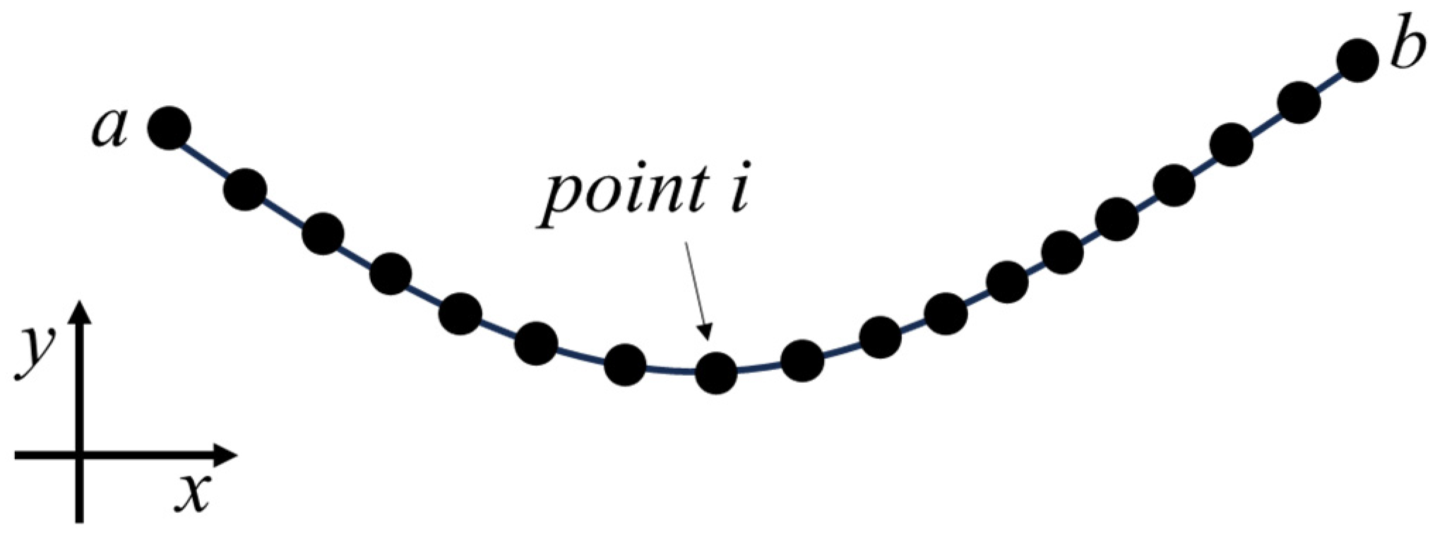
Figure 2.
Path unit of cable structure.
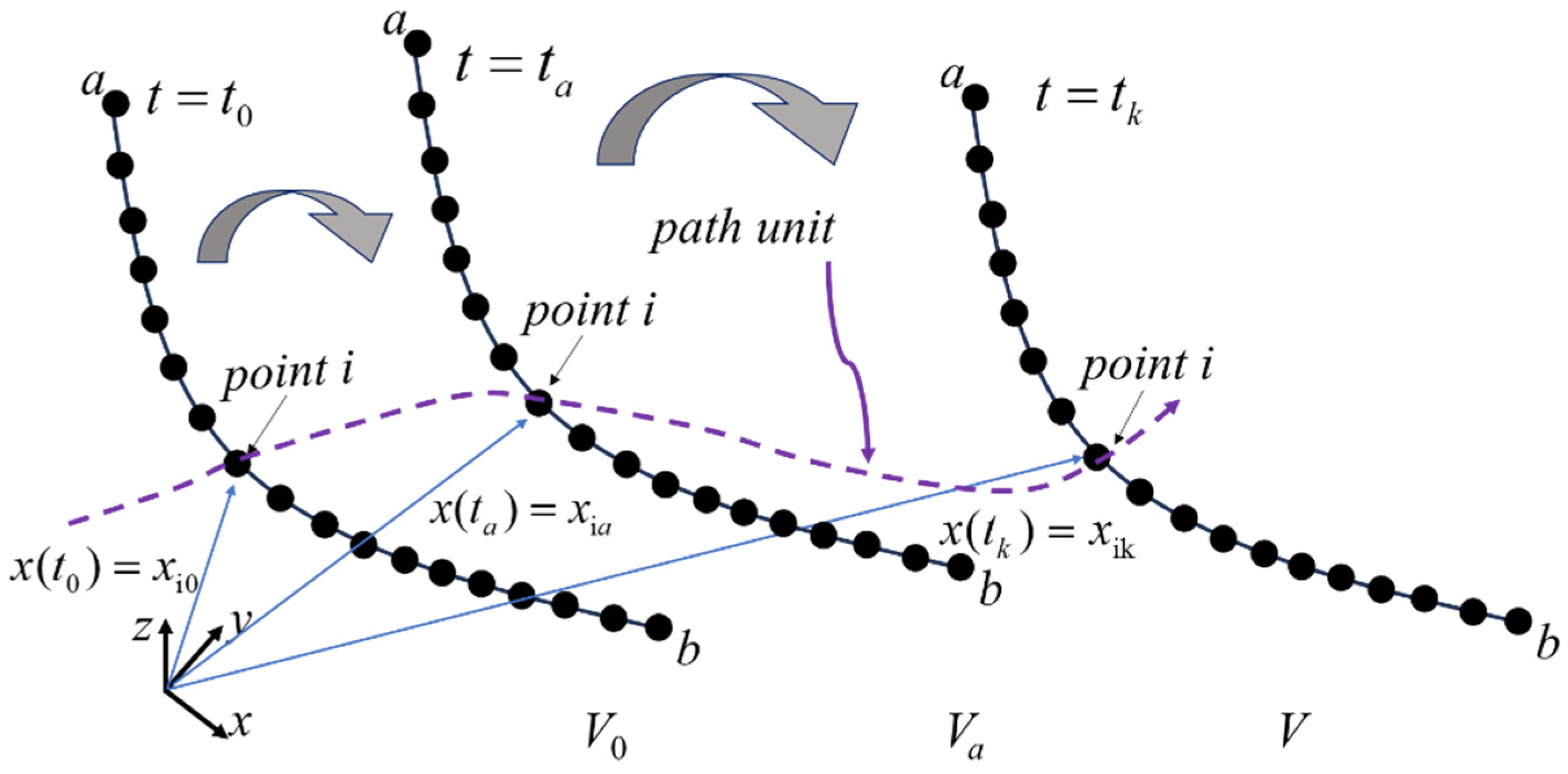
Figure 3.
Using ‘virtual motion’ to calculate the element deformation.

Figure 4.
Antenna cable net structure layout.

Figure 5.
Antenna Cable Net Discretization Strategy Based on FPM.

Figure 6.
Initial configuration of equilibrium state of cable net structure.
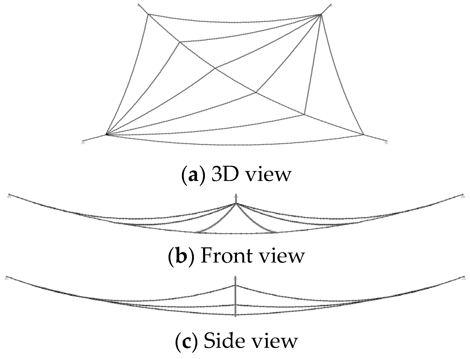
Figure 7.
Traverse sag calculation.
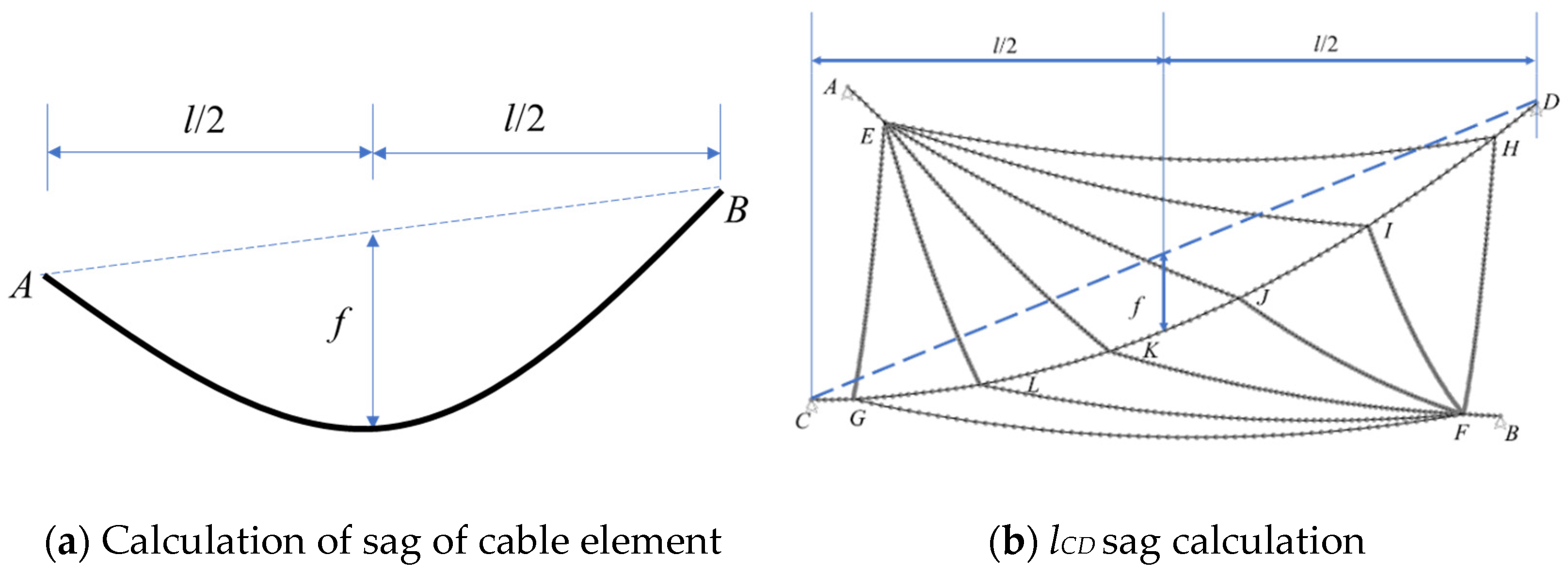
Figure 8.
Flow chart for aeolian-induced vibration analysis of large-span antenna net.
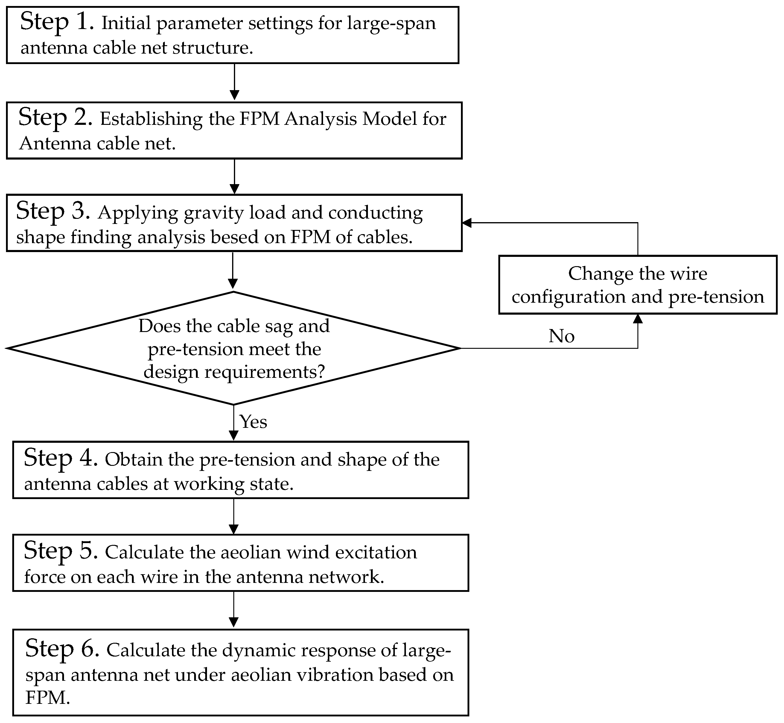
Figure 9.
Comparison of vibration response for mid-span particle.
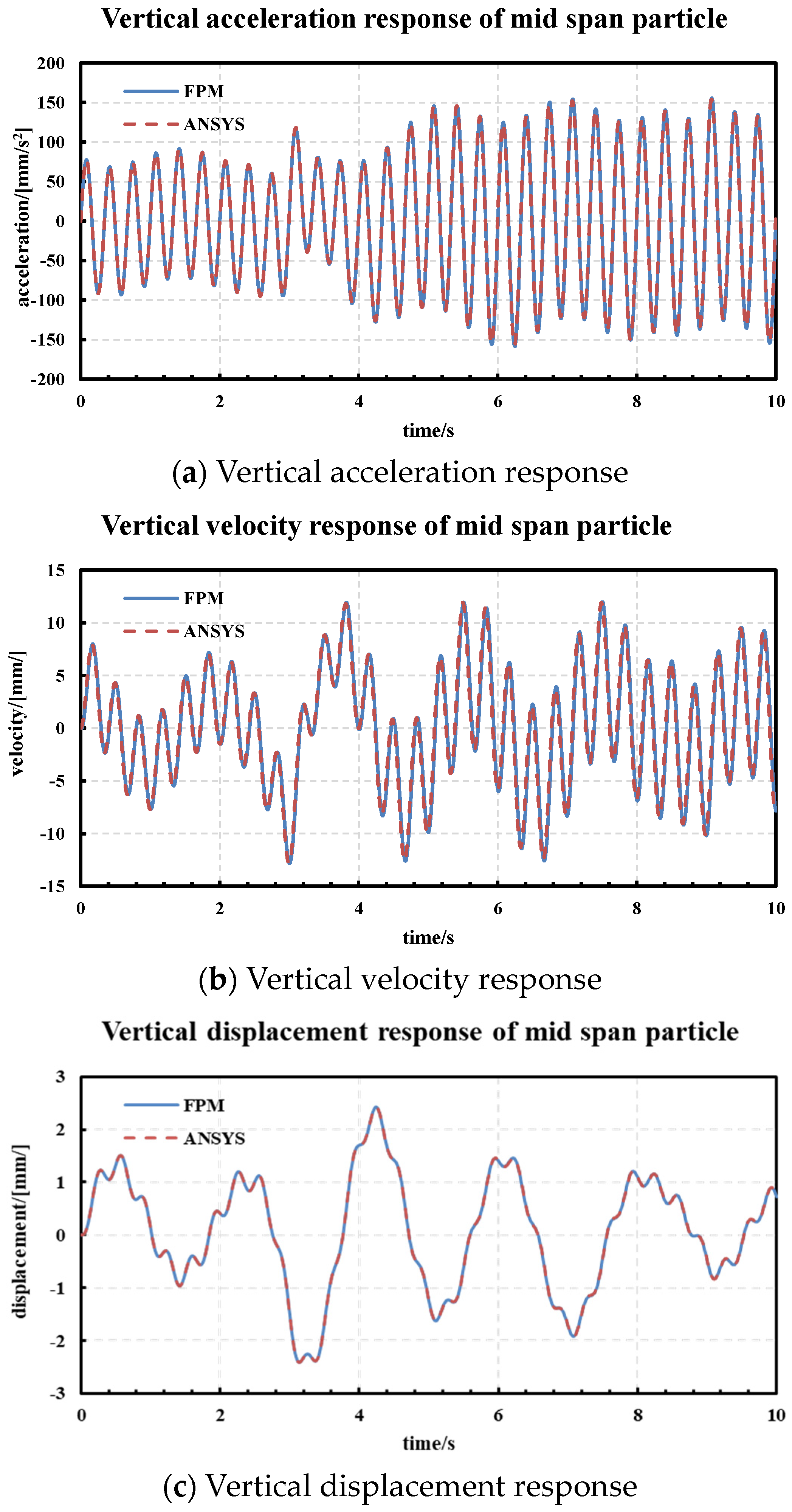
Figure 10.
Comparison of vibration response for mid-span particle.
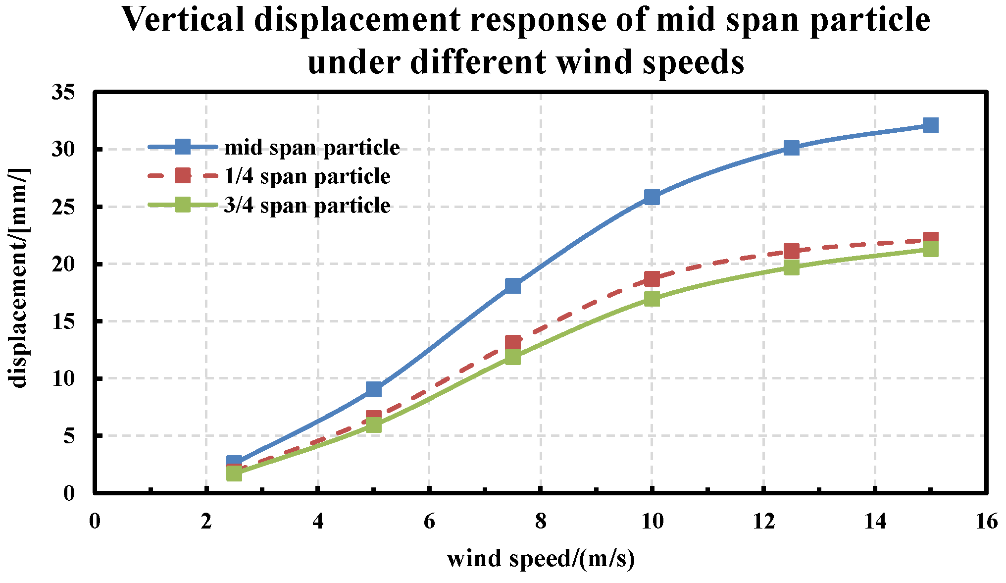
Figure 11.
Comparison of vertical displacement response along cable.


Table 1.
Mechanical information of wire materials.
| Number | Section Diameter (mm) | Section Area (mm2) | Elastic Modulus (N/mm2) |
|---|---|---|---|
| 1 | 40 | 1257 | 142,000 |
| 2 | 40 | 1257 | 142,000 |
| 3 | 40 | 1257 | 142,000 |
| 4 | 40 | 1257 | 142,000 |
| 5 | 30 | 707 | 61,700 |
| 6 | 30 | 707 | 61,700 |
| 7 | 30 | 707 | 61,700 |
| 8 | 30 | 707 | 61,700 |
| 9 | 30 | 707 | 61,700 |
| 10 | 30 | 707 | 61,700 |
| 11 | 40 | 1257 | 142,000 |
| 12 | 40 | 1257 | 142,000 |
| 13 | 40 | 1257 | 142,000 |
| 14 | 40 | 1257 | 142,000 |
| 15 | 40 | 1257 | 142,000 |
| 16 | 30 | 707 | 61,700 |
| 17 | 30 | 707 | 61,700 |
| 18 | 30 | 707 | 61,700 |
| 19 | 30 | 707 | 61,700 |
| 20 | 30 | 707 | 61,700 |
| 21 | 30 | 707 | 61,700 |
Table 2.
Initial equilibrium tension of wire.
| Cable Number | Wire Tension/kN | Cable Number | Wire Tension/kN | Cable Number | Wire Tension/kN |
|---|---|---|---|---|---|
| 1 | 173 | 8 | 38 | 15 | 193 |
| 2 | 238 | 9 | 31 | 16 | 27 |
| 3 | 173 | 10 | 27 | 17 | 31 |
| 4 | 237 | 11 | 193 | 18 | 38 |
| 5 | 27 | 12 | 157 | 19 | 38 |
| 6 | 31 | 13 | 141 | 20 | 31 |
| 7 | 38 | 14 | 157 | 21 | 27 |
Table 3.
Traverse sag.
| Number | Type | Sag | Number | Type | Sag |
|---|---|---|---|---|---|
| 1 | Sling | 0.35% | 12 | Sling | 1.21% |
| 2 | Sling | 0.26% | 13 | Sling | 1.35% |
| 3 | Sling | 0.35% | 14 | Sling | 1.21% |
| 4 | Sling | 0.26% | 15 | Sling | 0.96% |
| 5 | Top capacity line | 5.57% | 16 | Top capacity line | 5.57% |
| 6 | Top capacity line | 3.99% | 17 | Top capacity line | 3.99% |
| 7 | Top capacity line | 2.79% | 18 | Top capacity line | 2.79% |
| 8 | Top capacity line | 2.79% | 19 | Top capacity line | 2.79% |
| 9 | Top capacity line | 3.99% | 20 | Top capacity line | 3.99% |
| 10 | Top capacity line | 5.57% | 21 | Top capacity line | 5.57% |
| 11 | Sling | 0.96% | lCD | Sling | 8.67% |
Table 4.
First-order frequency of each wire.
| Number | Wire Length (m) | Mass per Unit Length of Wire (1 × 10⁻³ N·s2/m) | Initial Tension (kN) | 1st-Order Frequency (Hz) |
|---|---|---|---|---|
| 1 | 58 | 8.59 | 173 | 4.90 |
| 2 | 58 | 8.59 | 238 | 5.69 |
| 3 | 58 | 8.59 | 173 | 4.90 |
| 4 | 58 | 8.59 | 237 | 5.69 |
| 5 | 643 | 1.90 | 27 | 0.37 |
| 6 | 530 | 1.90 | 31 | 0.48 |
| 7 | 462 | 1.90 | 38 | 0.61 |
| 8 | 462 | 1.90 | 38 | 0.61 |
| 9 | 530 | 1.90 | 31 | 0.48 |
| 10 | 643 | 1.90 | 27 | 0.37 |
| 11 | 179 | 8.59 | 193 | 1.68 |
| 12 | 182 | 8.59 | 157 | 1.49 |
| 13 | 183 | 8.59 | 141 | 1.40 |
| 14 | 182 | 8.59 | 157 | 1.49 |
| 15 | 179 | 8.59 | 193 | 1.68 |
| 16 | 643 | 1.90 | 27 | 0.37 |
| 17 | 530 | 1.90 | 31 | 0.48 |
| 18 | 462 | 1.90 | 38 | 0.61 |
| 19 | 462 | 1.90 | 38 | 0.61 |
| 20 | 530 | 1.90 | 31 | 0.48 |
| 21 | 643 | 1.90 | 27 | 0.37 |
Table 5.
Comparison of calculation results.
| Comparison Item | FPM | ANSYS | Relative Error |
|---|---|---|---|
| Maximum vertical acceleration response (mm·s−2) | 156.39 | 158.20 | 1.14% |
| Maximum vertical velocity response (mm·s−2) | 12.82 | 12.79 | 0.20% |
| Maximum vertical displacement response (mm·s−2) | 2.42 | 2.43 | 0.42% |
Disclaimer/Publisher’s Note: The statements, opinions and data contained in all publications are solely those of the individual author(s) and contributor(s) and not of MDPI and/or the editor(s). MDPI and/or the editor(s) disclaim responsibility for any injury to people or property resulting from any ideas, methods, instructions or products referred to in the content. |
© 2023 by the authors. Licensee MDPI, Basel, Switzerland. This article is an open access article distributed under the terms and conditions of the Creative Commons Attribution (CC BY) license (https://creativecommons.org/licenses/by/4.0/).
Share and Cite
MDPI and ACS Style
Qin, K.; Zhao, F.; Luo, Y.; Fang, B.; Chen, S. Aeolian Vibration Dynamic Analysis of Large-Span, Relaxed Antenna Cable Net Based on Finite Particle Method. Buildings 2024, 14, 105. https://doi.org/10.3390/buildings14010105
AMA Style
Qin K, Zhao F, Luo Y, Fang B, Chen S. Aeolian Vibration Dynamic Analysis of Large-Span, Relaxed Antenna Cable Net Based on Finite Particle Method. Buildings. 2024; 14(1):105. https://doi.org/10.3390/buildings14010105
Chicago/Turabian StyleQin, Kai, Fan Zhao, Yaozhi Luo, Bin Fang, and Shangyuan Chen. 2024. "Aeolian Vibration Dynamic Analysis of Large-Span, Relaxed Antenna Cable Net Based on Finite Particle Method" Buildings 14, no. 1: 105. https://doi.org/10.3390/buildings14010105
Note that from the first issue of 2016, this journal uses article numbers instead of page numbers. See further details here.