Article

Determination of the Effective Elastic Modulus for Nodular Cast Iron Using the Boundary Element Method

1
Group of Experimental and Computational Mechanics, University of Brasília, 72.405-610 Gama, Brazil
2
Engineering School, Fluminense Federal University, Rua Passo da Patria 156, 24210-240 Niterói, Brazil
3
Institute of Computing, Fluminense Federal University, Rua Passo da Pátria 156, 24210-240 Niterói, Brazil
*
Authors to whom correspondence should be addressed.
Metals 2018, 8(8), 641; https://doi.org/10.3390/met8080641
Submission received: 21 June 2018 / Revised: 20 July 2018 / Accepted: 21 July 2018 / Published: 15 August 2018
(This article belongs to the Special Issue Cast Irons: Properties and Applications)

Abstract

:
In this work, a multiscale homogenization procedure using the boundary element method (BEM) for modeling a two-dimensional (2D) and three-dimensional (3D) multiphase microstructure is presented. A numerical routine is specially written for modeling nodular cast iron (NCI) considering the graphite nodules as cylindrical and real geometries. The BEM is used as a numerical approach for solving the elastic problem of a representative volume element from a mean field model. Numerical models for NCI have generally been developed considering the graphite nodules as voids due to their soft feature. In this sense, three numerical models are developed, and the homogenization procedure is carried out considering the graphite nodules as non-voids. Experimental tensile, hardness, and microhardness tests are performed to determine the mechanical properties of the overall material, matrix, and inclusion nodules, respectively. The nodule sizes, distributions, and chemical compositions are determined by laser scanning microscopy, an X-ray computerized microtomography system (micro-CT), and energy-dispersive X-ray (EDX) spectroscopy, respectively. For the numerical model with real inclusions, the boundary mesh is obtained from micro-CT data. The effective properties obtained by considering the real and synthetic nodules’ geometries are compared with those obtained from the experimental work and the existing literature. The final results considering both approaches demonstrate a good agreement.

1. Introduction

The multiscale homogenization procedure for microstructural material is an important topic in the science and engineering of materials. According to Nguyen et al. [1], computer modeling is the most efficient technique for this purpose, and it has been a subject of interest in recent years. One of the main challenges for multiscale modeling is in developing numerical models that predict the behavior of microstructures with high accuracy and efficiency. Many works on this subject have been developed over the years [2,3,4,5]. According to Pundale et al. [6], microstructural materials are considered to be composites for the numerical modeling approach, where the challenge relies on coupling the individual behavior of each constituent to obtain an overall response.
Achenbach and Zhu [7,8] carried out numerical studies with multiphase media using a unit cell model to study the variation of the interface parameters and to estimate the effect of distribution of stresses in both the matrix and in the fibers. Moorthy and Ghosh [9] developed a finite element (FE) model in conjunction with Voronoi cells to examine the small deformation of arbitrary heterogeneous material in a 2D model. The influences of the shape, size, orientation, and distribution of inclusions on the micro- and macroscopic responses were also investigated. The results indicated that the orientation of every grain did not play as important a role as the size of the inclusions in the response of the overall properties.
Effective properties of macrostructural materials using synthetic geometries (i.e., regular geometries such as cylinders, spheres, and ellipsoids) of different sizes and different mechanical properties were studied by Yao et al. [10], who used a 2D formulation in the boundary element method (BEM) to demonstrate that the BEM formulation may be more suitable for interface analysis when compared to the FE method. Using the following two approaches, Zheng et al. [11] studied a solid whose macrostructure comprised fluid-filled pores: the superposition method and a multi-subdomain method 2D BEM model using subregions. It was shown that the multi-subdomain method (with subregions) was more efficient and accurate for determining the effective properties. Gitman et al. [
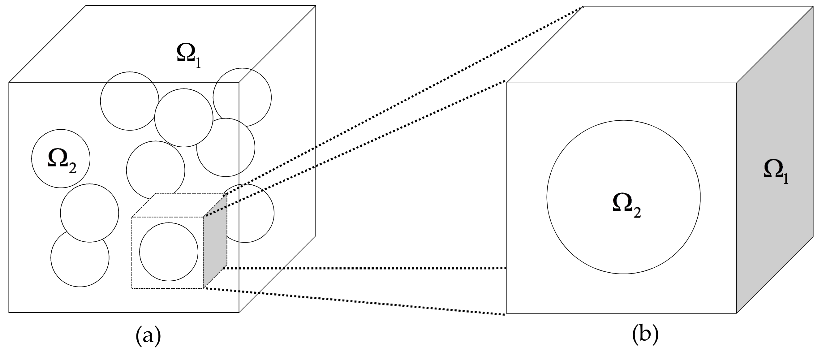
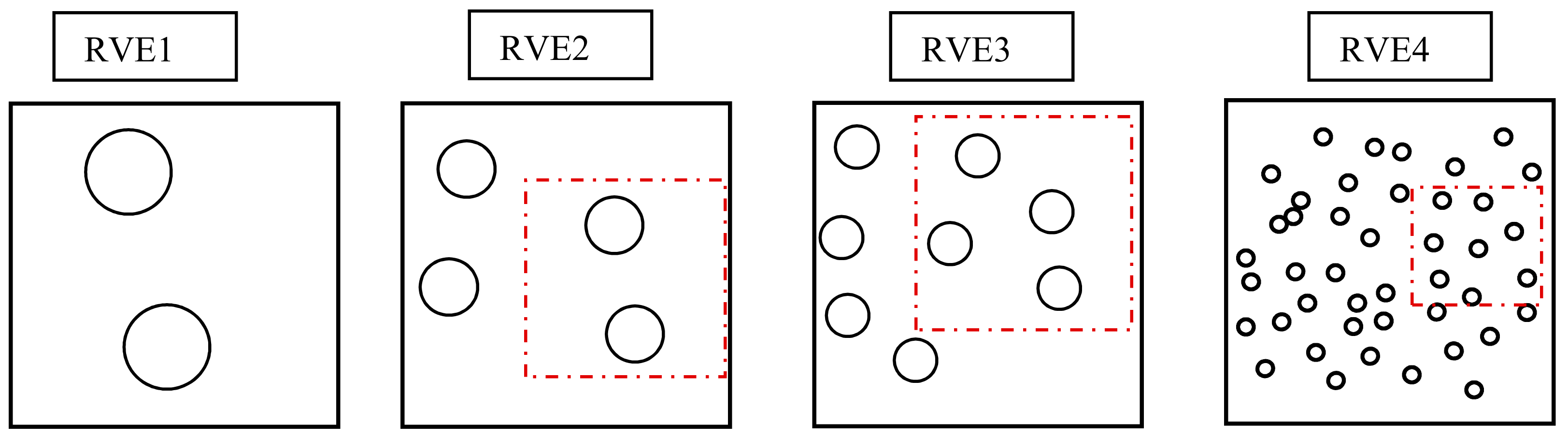
12] discussed the periodicity of the material, and they established the no-wall-effect concept, which refers to the inability of inclusions to penetrate through the sample borders within a representative volume element (RVE). According to Gitman [12], the periodicity of a material considers that a material experiencing no-wall effects due to the RVE is a representative volume and should, therefore, represent any part of the material. Despite the many experimental and computational methods devoted to the study of the effective elastic modules of nodular cast iron (NCI) [6,13,14,15], it is important to highlight that computational methods are much more attractive from the point of view of saving time and reducing the operational costs.
Numerical homogenization was used based on the concept of the RVE for determining the effective properties. Through this method, the statistical data of many RVEs can be obtained, and by averaging the values of each distribution of spherical inclusions, it is possible to find the global response of the material [16]. According to Zohdi [16], this technique is more trustworthy than performing individual direct simulations. Buroni and Marczak [13] developed a homogenization procedure using a 2D BEM as a numerical approach to determine the effective modulus of NCI. In this work, the inclusions were considered to be voids, which were discretized with a single special hole element. This new numerical approach demonstrated good accuracy and low computational cost. Carazo et al. [17] performed an RVE study to determine the effective properties of NCI. The authors imposed rectangular and hexagonal geometric shapes of the RVE; the numerical results were compared to analytical expressions, and the authors concluded that the graphite fraction has the largest influence on the effective modulus. They realized that the effective properties are independent of the RVE shape. Fernandino et al. [15] recently used the FE method and a multiscale analysis to determine the effective elastic proprieties of NCI where a complete experimental characterization was introduced and used to evaluate the numerical results.
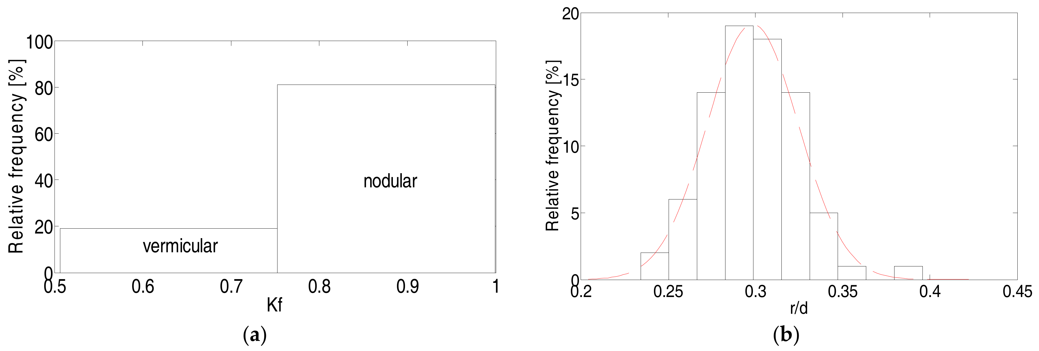
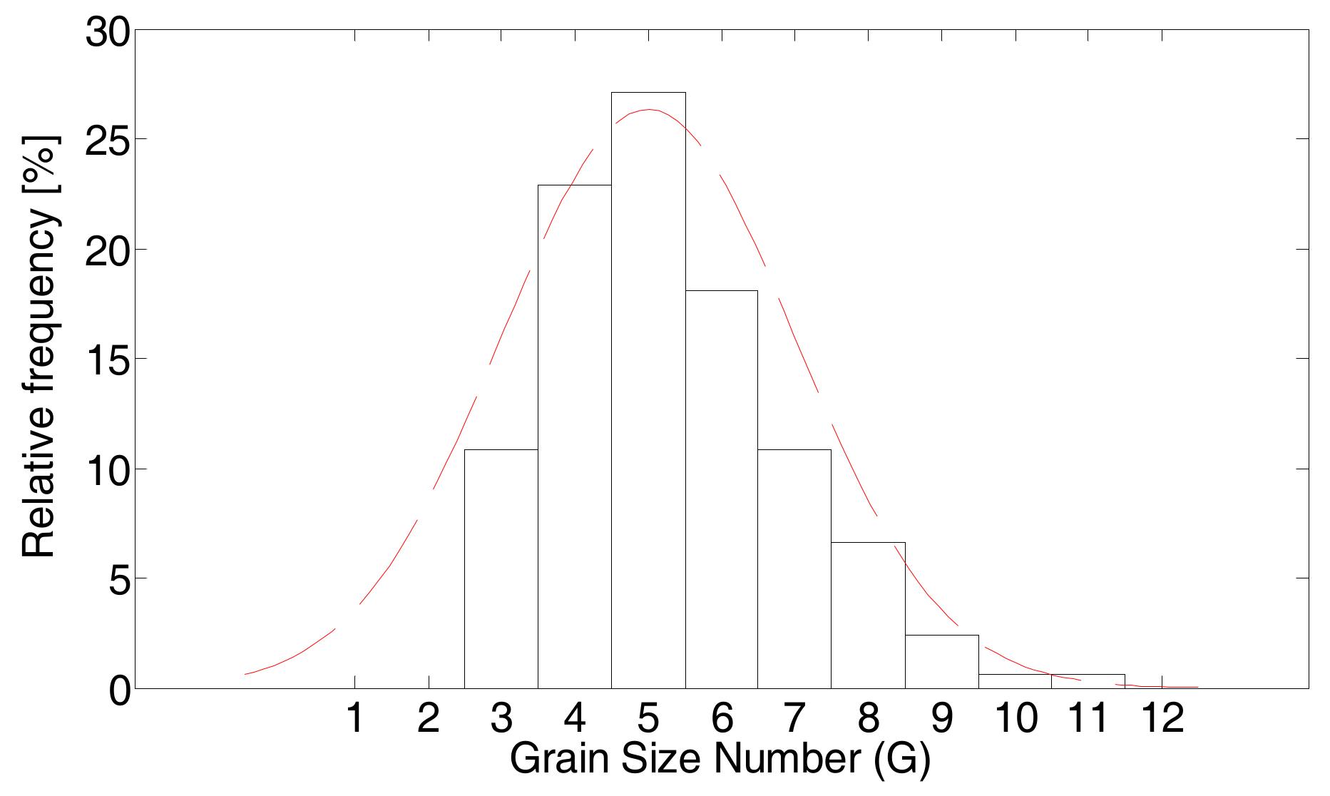
In this paper, the main objective is to develop a homogenization process for NCI. Nodular cast iron, also known as spheroidal graphite cast iron (SGI), was chosen to develop a numerical model of homogenization. The main reason is the morphology of the microstructure, which contains nearly spherical inclusions of graphite embedded in a homogeneous ferritic matrix. The nodular graphite has a high carbon content, while the matrix medium has a ferritic, pearlitic, ferritic-pearlitic, or austenitic structure [
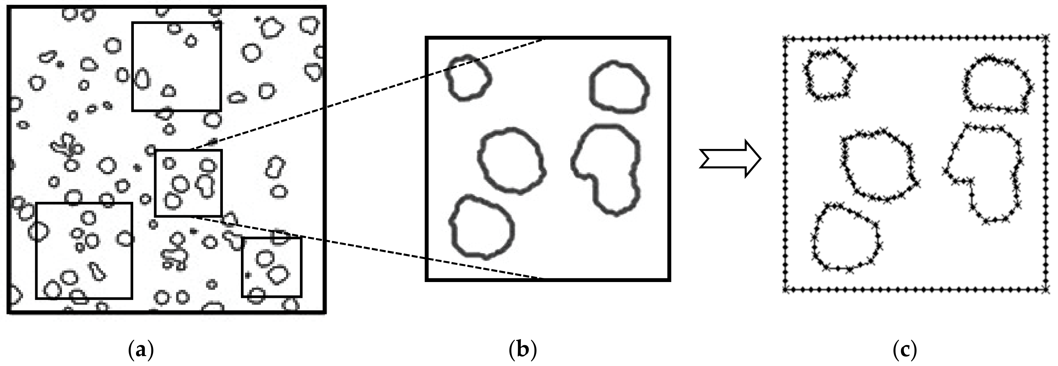
18]. For the numerical homogenization process, two approaches were employed: the first one models the nodules as a synthetic geometry, and the second one models them as their real shapes obtained via microtomography. A numerical routine using the BEM for the homogenization analysis was supported by experimental studies, such as microtomography by X-rays (micro-CT), tensile tests, hardness tests, microhardness tests, micrographic analyses, and scanning electron microscopy equipped with energy-dispersive X-ray (SEM-EDX) analyses. The main goal of this investigation is to determine the influence on the effective properties obtained when considering the nodules as synthetic and real geometries in the homogenization process.

2. Numerical Model

A multiscale numerical routine was written based on the BEM as the numerical approach for determining the effective Young’s modulus of heterogeneous materials with linear elastic behavior. The graphite was modeled as a second constituent by using the subregion methodology provided by BEM. The subregion formulation takes into account the stiffness of nodular inclusions within the ferritic homogeneous matrix of NCI. To accelerate the convergence of the homogenization process, periodic boundary conditions were also implemented in the numerical routine, particularized to plane stress (PT).

2.1. The BEM and Subregions

The BEM is essentially based on the domain’s boundary, which is partitioned in a coarse mesh where the differential governing equation is numerically integrated [19,20]. This numerical approach has all the unknown variables only on the boundary, meaning that no information from inside the domain is required. Figure 1 illustrates a boundary value problem considering both an RVE by sub-region and a no-wall-effect concept [12]. The ferritic matrix is denoted by the subscript 1, and the graphitic nodules are indicated by the subscript 2.
The governing equation for a linear elastic material is presented in Equation (1):
u ( x ) = Γ i U i j ( x , y ) t ( y ) t ( y ) d s y Γ i T i j ( x , y ) u ( y ) d s y
where U and T are the components of displacement and tractions containing the fundamental solutions for the nodal displacement (u) and tractions (t), respectively. The fundamental solutions for a 2D elastic model are as follows:
U i j ( x , y ) = 1 8 π μ [ ( 3 4 ν ) log 1 r δ i j + r i r j ]
T i j ( x , y ) = 1 4 π ( 1 ν ) r { r n [ ( 1 2 ν ) δ i j + 2 r i r j ] + ( 1 2 ν ) ( n i r j n j r i ) }
where μ and ν are the shear stress and Poisson’s ratio, respectively; r is the distance between the source point and a field point; and δ stands for the Kronecker delta. Once the external boundary conditions are imposed, the system is integrated over the total number of nodes (Tn), resulting in a linear system of equations:
i = 1 T n [ H i j u i ] = i = 1 T n [ G i j t i ] [ H ] ( u ) = [ G ] ( t )
where H and G are the arrays of displacement and tractions, respectively. Every subregion is discretized by discontinuous quadratic elements. Therefore, the BEM equations for each subregion were implemented according to Brebbia and Dominguez [19] and Aliabadi [20].
For the homogenization process to succeed, the influence of the boundary conditions imposed on the problem must be taken into account in order to increase the accuracy and convergence. In this sense, three classical methods may be used to impose the boundary conditions [21]: (1) a linear displacement boundary condition (Dirichlet condition); (2) a constant traction boundary condition (Neumann condition); and (3) a periodic boundary condition (PBC). Some works [21,22,23] emphasize the importance of imposing the PBC due to its efficiency and accuracy for the final results of analyses in microstructural material. In this work, a PBC that considers the Dirichlet condition was implemented to ensure good accuracy in the homogenization procedure.

2.2. Constitutive Law

The constitutive linear equation of an elastic material is written in index notation as:
σ i j = C i j k m ε k m
where Cijkm represents the components of the fourth-order constitutive tensor, which relates the stress and strain tensors, and it is related to the mechanical properties according to Equation (6):
C i j k m = E 1 ν 2 [ ( 1 ν ) I i j k m + ν ( I i j × I i j ) ]
where E and ν denote the Young’s modulus and Poisson’s ratio, respectively. In our problem using subregions, these parameters are given by:
E = { E m a t r i z a n d ν m a t r i z i f    ( x , y ) Ω m a t r i x E n o d u l e a n d ν n o d u l e i f    ( x , y ) Ω n o d u l e
where Ematrix and νmatrix are the Young’s modulus and Poisson’s ratio, respectively, for the ferritic matrix, while Enodule and νnodule are the Young’s modulus and Poisson’s ratio for the graphite nodule.

2.3. The Plane Stress (PT) and Plane Strain (PS) Hypotheses and the Mean Field Theory

The PT and PS hypotheses are two considerations that should be taken into account to decrease the computational costs as well as to minimize the number of variables for a 2D analysis. The macroscopic properties of a heterogeneous material are typically determined using Equation (8), where the micro- and macro-couplings are implicitly defined. Equations (9) and (10) establish the relationship between the infinitesimal macroscopic stress and strain tensors and the averages of the stress and strain in the RVE [24]:
σ i j Γ = C i j k m ε k m Γ
ε i j M = ε i j Γ
σ i j M = σ i j Γ
where ‹› stands for the average stress taken over the boundary Γ. It is the spatial average operator, which is defined as follows:
= 1 | Γ | Γ d Γ
when is the mechanical property to be evaluated. According to Zohdi et al. [25], a specimen can be computationally tested to permit the solution to the elastic problem for determining the stress and strain micro fields. Solving the system of equations shown in Equation (8) determines the constants for the matrix of elasticity. The microstructural sample material is subjected to the same boundary conditions, resulting in a field of tensions and deformations that are distributed uniformly as an entire homogeneous body [13,24].

3. Methodology and Materials

In this work, the graphite nodules were modeled numerically using two different procedures. The first one employs a statistical analysis, assuming that nodular graphite has a synthetic geometry (circular shape), and the second procedure assumes that the nodular graphite has the real geometry obtained by X-ray microtomography. The morphological characterization and mechanical properties were determined through experimental tests, which were used to support and validate the proposed numerical homogenization.

3.1. X-Ray Microtomography

To validate the proposed methodology, digital images were acquired using micro-CT. The samples were scanned using a ZEISS X radial 510 Versa, high-resolution, micro-CT scanner system (Versa 510, Bregnerødvej, Birkerød, Denmark). This system generates X-rays with a cone-beam geometry, and a 3D digital object can be visualized from the acquired radiograms. The small samples of NCI have dimensions of 6 mm × 7 mm × 24 mm. Each sample was then mounted on a rotating cylindrical support inside the X-ray chamber and positioned so that the X-ray lines were perpendicular to their axis of rotation. Then, the scanning parameters were adjusted and scanned for 15 s. The geometry obtained by micro-CT was straightforwardly exported to generate a BEM mesh, making it possible to use the real geometry of the microstructure.
Through the micro-CT images, it was also possible to determine the shape coefficient K f ( K f = D 1 / D 2 ) and the characteristic parameter r / d ( r = ( D 1 + D 2 ) / 4 ) . Here, D 1 and D 2 are the smallest and the largest diameter, respectively, measured inside the graphite nodule; r is the average radio; and d is the average distance measured between two graphite nodules [26,27].
To obtain an approximate representation of the characteristic parameters of the NCI microstructure, a statistical analysis was implemented by random selection of graphite nodules over the analysis zone. All data were tabulated in histograms.

3.2. Microstructure of NCI

A micrographic analysis was used to characterize the spatial distribution of graphite nodules and the average nodule size. Micrograms were obtained from NCI blocks with dimensions of 5 mm × 5 mm × 5 mm. The surface was polished and etched with nital at 3%, and the samples were then mounted on a sample holder and analyzed in a vacuum according to ASTM E112-96 standard. Three micrograms were obtained with scales of 400, 100, and 20 μm, and the resulting images were used to measure the amount, area, and overall size of the graphite nodules.

3.3. Hardness Tests

Vickers and Brinell hardness testing was performed to measure the hardness of both the ferritic matrix and the graphite nodules in line with ASTM E92-16 standard. By using the micro-indentation methodology [28], it was possible to determine the Young’s modulus for both the matrix and the graphite nodules. In this work, the measurements were carried out with an FM 700 Vickers microhardness apparatus (FM 700 Vickers, Karola Miarki 12, Gliwice, Polska), equipped with a glass camera with a 100 × magnification capability and which had a load of 10 g. The average hardness of the ferritic bulk was determined using a Brinell hardness (HB) test, in line with ASTM E92-16, with a semiautomatic HB tester (ZHU250 HB, Kennesaw, GA, USA). Afterwards, the tensile strength of NCI was determined through the standard correlations between the HB hardness and tensile strength. Figure 2a,b depict the shallow indentations made in the microhardness tests, revealing that the graphite nodule is softer than the matrix due to the difference in highlights between the areas of the hardness impression. The HB test is presented in Figure 2c. In this case, the spherical indentations are larger than the Vickers hardness HV indention, meaning that the hardness value only indicates the toughness of the bulk material.
The mathematical model discussed in [28] consists of identifying the geometric parameters of the indented surface. Then, from the geometrical parameters of the hardness impressions and the mechanical and geometrical properties of the indenter, it is possible to determine the Young’s modulus according to Equation (12):
E = 1 υ 2 1 E r 1 v i 2 E i
where νi is the Poisson’s ratio of the indenter, ν is the Poisson’s ratio of the sample, Ei is the Young’ modulus of the indenter, Er is the reduced Young’s modulus of the sample, and E is the Young’s modulus of the sample. The parameters used for estimating the effective Young’s modulus are listed in Table 1.
The values of Er were extracted by using Equation (13):
E r = ϖ P max π 2 h s A
where ϖ is a constant that depends on the geometry of the indenter; Pmax is the maximum load; hs is the amount of sink-in, which is assumed to be approximately equal to the final depth hf; and A is the projected area of the elastic contact. Due to the uncertainty in the Vickers system and the structurally inhomogeneous sample, a statistical test was developed using micro-indentation patterns containing 50 indentations over the analysis zone.

3.4. Tensile Tests

Tensile testing was performed on sub-size test samples, which were obtained by machining the NCI blocks according to the specifications in ASTM E8/E8M-09 standard, using an Instron 8801 test machine (Instron, Glenview, IL, USA) [±100 kN (22,500 lbf)] with a 2620-601 dynamic gauge extensometer (Instron, Glenview, IL, USA). The Young’s modulus, tensile strength, and ultimate tensile strength were determined from the experimental stress-strain curve.

3.5. Scanning Electron Microscope Equipped with EDX

The quantitative compositional information for NCI was determined by using a scanning electron microscope system equipped with energy dispersive X-ray analyzer system (JEOL JSM 6610 SEM-EDX, Musashino, Tokyo, Japan). The samples were polished, treated, and placed in a vacuum chamber for visualization of the surface. The samples were analyzed at 100×, and the microstructural examinations were carried out for a representative sample with a large number of graphite inclusions.

3.6. Computational Homogenization

The homogenization concept is based on a multiscale analysis that establishes the relationships between macro- and micro-scale entities [29]. The micromechanical analysis typically focuses on the concepts of RVEs; the analysis involves an average representative volume extracted from the micro-heterogeneity in an infinitesimal-volume sample [1,12,24]. This sample contains a reasonable representation of the microstructure’s material; therefore, the material properties are obtained through average volumes of the respective micro fields obtained from an RVE [12,24]. The numerical homogenization was developed following two procedures.

3.6.1. Case I: Graphite Nodules Considered as Synthetic Geometry

The synthetic homogenization procedure was developed using the characteristic parameters obtained from statistical analyses based on morphological characterizations. There is no definitive way in which to establish an RVE [16].; the most frequently used procedure currently involves either fixing the nominal RVE size and then increasing the number of graphite nodules (Figure 3) or increasing the size of the RVE so that the number of heterogeneities changes by a fixed percentage.
In Figure 3, RVE1 ⊂ RVE2 ⊂ RVE3 ⊂ RVE4. The discretization strategy of the microstructure was assumed to be a square sheet for the 2D RVE case and a cube for the 3D RVE case. In both cases, a constants dimension, containing a specific number of nodules, was defined. The characteristic parameter obtained with the procedure described in Section 3.1 was used to model NCI. The nodules/matrix ratio of the sample was obtained by morphological characterization using image analysis during the binarization process, which establishes the percentage of each phase. The homogenization model employed samples with the following numbers of nodules: 4, 6, 8, 10, 15, 20, 25, 30, 40, 45, 50, 55, and 60.

3.6.2. Case II: Graphite Nodules Considered as Real Geometry

Figure 4 presents the homogenization procedure used to estimate the effective Young’s modulus considering a real morphology. This procedure involves the generation of several RVEs with different sizes and in random coordinates over the sample (Figure 4a) [12]. The RVE sizes were obtained from numerical tests, where constant displacements were imposed as a boundary condition. Furthermore, the micrograms obtained by micro-CT were used to obtain the forms and distribution of the nodules (Figure 4b). In the sequence, a 2D mesh that represents the inclusions of the irregular geometry inside the ferritic matrix was generated (Figure 4c).
The boundary was discretized with a discontinuous quadratic element. Moreover, the dimensions of the RVE were progressively increased until the effective Young’s modulus was reached.

4. Results and Discussion

The results obtained from the experimental and numerical tests described in the previous section are presented below.

4.1. X-Ray Microtomography

According to the micro-CT images, the graphite nodules exhibited a shape that is approximately a circle. In this sense, the shape parameter (Kf) and the characteristic parameter (r/d) were estimated through statistical testing. Figure 5 illustrates the nodule distributions in an NCI sample. The results for Kf and the r/d ratio are presented in a histogram graph.
According to Figure 5a, it is possible to verify that the graphite nodules present a dominant circular shape, as most of the samples present Kf values between 0.75 and 1.0. However, some inclusions also present a vermicular shape. Due to this accentuated characteristic, in this work, the homogenization procedure using synthetic geometry will be developed considering the graphite as a circular shape. The r/d parameter was 0.3 ± 0.01, as indicated in Figure 5b, and the error was sufficiently low for the model representation of NCI. These parameters were coded into the numerical model to represent NCI.

4.2. Microstructure of NCI

The micrograms obtained from the laser confocal system were used to determine the NCI grain size. Figure 6 presents the microstructure of a sample of NCI after etching with a 3% nital solution. In Figure 6a, the ferritic-pearlitic structure of the sample is observed. This structure is surrounding the nodular graphite, forming a so-called “bullseye,” and it contains certain alloying elements, such as magnesium and silicon, and small quantities of other elements that do not act during the nucleation process. The presence of pearlite lamellae is due to the high cooling rate of the iron from the eutectoid temperature. Figure 6b depicts the matrix structure with the “bullseyes” and the mixture of fine lamellar pearlite and a ferrite matrix structure. Finally, Figure 6c presents the pearlite as a thin lamellar structure, which is the result of a high cooling rate after casting. Graphite is surrounded by perlite, with the presence of some ferrite [30].
Table 2 summarizes the result for NCI that corresponds to the nodule diameter for a grain size number (G) of 4.62 (See ASTM E112-96). The average grain size of NCI obtained from the statistical count is illustrated in Figure 7.
From Figure 7, the nodular graphite size indicates a value of G of around 5. In addition, ASTM E112-96 standard presents a relationship between G and the average diameter. For this study, the average diameter is approximately 64 ± 10 μm, which is in good agreement with related works [18,31,32].

4.3. Hardness Tests

The effective Young’s modulus was determined from the Vickers micro-hardness tests, with the associated results presented via the histograms in Figure 8a,b for the Young’s modulus of the matrix and the nodules, respectively.
The mean and standard deviations for the matrix and nodules are 241 ± 19   GPa and 29.17 ± 1.1   GPa , respectively. There is a significant difference between the Young’s modulus of the matrix and that of the graphite nodules; the main reason for this is the low strength of the graphite. To ensure that the present results are valid, some studies regarding the determination of the Young’s modulus for NCI are introduced and presented in Table 3.

4.4. Tensile Tests

Tensile tests were performed, and the stress versus strain curve is presented in Figure 9. The mechanical properties, including the yield stress (σ0.2), ultimate tensile strength (σu), Young’s modulus (E), and Poisson’s ratio (ν), were obtained from the experimental curve, and they are reported in Table 3. The Young’s modulus was 171 GPa, averaged over the four tests. The values of the modulus of elasticity that others obtained for NCI are 187 GPa [33], 172 GPa [15], and 179 GPa [34], demonstrating good agreement with the present values.

4.5. Scanning Electron Microscope Equipped with EDX

During the formation of the nodular graphite in the casting process, additional elements, such as silicon and magnesium, are required to alter the solidification mechanism and chromium to improve the tensile strength. The chemical composition is presented in Table 4.
Nodular cast iron is formed by approximately 3.6% carbon, and it makes up 92.8% per mass of iron. The remaining chemical compounds were measured by SEM-EDX equipment (JEOL JSM 6610 SEM-EDX, Musashino, Tokyo, Japan). Despite obtaining information regarding all percentages of constituents (Table 4), it is important to note that this type of equipment is not able to detect small percentages of chemical constituents with good accuracy. For those constituents with high percentages (Fe, Si, and C), the values measured through the use of SEM-EDX equipment demonstrated good agreement with those provided by the foundry industry from which these samples were acquired. The high amounts of carbon are responsible for the formation of nodular graphite and for the lamellar perlite produced by the carbon remainder that did not form graphite during nucleation. According to Table 4, the high percentage of Si joined to the Mg explains the nodular graphite’s round shape in the ferritic matrix. The small amounts of Cr and Cu account for the formations of the pearlite structure and the high tensile strength.

4.6. Computational Homogenization

4.6.1. Case I: Graphite Nodules Considered as Synthetic Geometry

Two-Dimensional Model

Figure 10 illustrates the convergence curve for E*, where a wide dispersion for each computational test is evidenced. According to this graph, when a few nodules are considered, E* varies considerably, indicating a positional dependence, which affects the effective properties significantly. It is possible to observe that as the number of nodules increases, E* stabilizes for each set of samples. The elasticity modules, as well as the statistical data, are presented in Table 5.
In Table 5, E* is the average value for each sample, (EmaxEmin) is the difference between the maximum and minimum values, (SD) is the standard deviation, (DVM) is the percentage deviation of the difference between maximum and minimum values with respect to the average, and (DM) is the percentage deviation of the standard deviation from the average value. Based on Table 5, it is possible to realize that E* is reached with 35 nodules, and after this increment, the Young’s modulus no longer varies significantly (less than 5%) except for particular points that affect the general result generated, as can be seen in Figure 11a. Figure 11a depicts the results for the E* microstructures containing 35 nodules in each analysis; the maximum, minimum, average, and standard deviations of the group of samples tested are shown. Figure 11b presents the corresponding histograms of the results, where most of the analyses yielded values for E* of 181 GPa. The value of E* for the NCI obtained from the experimental data is 171 GPa.
The slight difference between the experimental and numerical results is approximately 8%. This difference is perhaps due to the 2D microstructural model employed and its simplification. According to Rodrígues et al. [14], a difference exists in the effective properties when using 2D and 3D RVEs. The authors claim that hydrostatic effects on the deformation of a 2D nodule are different from those effects that occur in a real 3D solid.

Three-Dimensional Model

In this work, the same strategy from [13] and [16] was used to study the effective property in an NCI RVE. Figure 12 presents the convergence curve of E* for a 3D model. Furthermore, Table 6 lists the (EmaxEmin), the standard deviation, the percentage change in the difference between the maximum and minimum values with respect to sock (DVM) and the mean values of each of the samples for E*, and the difference between the maximum and minimum values and the standard deviation (DM).
It can be observed that an E* is reached for 30 inclusions, where there are increases of less than 5%. Figure 13a presents the result for E* for an RVE with 30 random distributions of inclusions, while Figure 13b presents the corresponding histograms of the results, where it can be appreciated that the data for E* were 186 GPa.
Now, for the 3D analysis, it can be seen that the Young's modulus was 186 GPa due to the hydrostatic effects that generate a higher stiffness in the material.

4.6.2. Case II: Graphite Nodules Considered as Real Geometry

The homogenization was performed through the use of the real geometry of the NCI microstructure obtained by micro-CT acquisition. The results of the homogenization process are presented in Figure 14. It can be observed that as the number of inclusions increases, the effective Young’s modulus is stabilized, reaching values of 175 GPa for an RVE with 30 inclusions. The RVE size in this case was 1.5 mm2. The present methodology demonstrated good accuracy for determining the effective Young’s modulus in relation to the values obtained with the experimental results, where the difference is approximately 8%. The error in the Young’s modulus value can be justified by the 2D model approach. Despite considering the real geometry of the graphite, a difference of 8% remains between the values of the effective Young’s modulus obtained experimentally and numerically. In this sense, perhaps a 3D model that takes into account the real geometry should be more realistic, thereby minimizing this difference. Table 7 summarizes the results for the effective Young's modulus obtained through homogenization (real and synthetic geometries) and the experimental procedure and those available in the literature.
In this work, three numerical models for determining the effective Young’s modulus were considered. Table 7 summarizes the results for the effective Young’s modulus obtained for each numerical model, the Young’s modulus obtained by tensile test. Considering the approach of the graphite nodule as a synthetic geometry, both 2D and 3D models resulted in values greater than those obtained experimentally and those available in the literature. However, the 2D model that considers the real geometry of a graphite nodule resulted in good agreement with the values obtained experimentally and with [33]. In this sense, it may be possible to claim that those models that consider the real geometry of graphite nodules are more accurate for determining the effective properties.

5. Conclusions

In this paper, a homogenization process for determining the effective Young’s modulus of NCI was performed. A numerical strategy for the homogenization process was written for a 2D and a 3D elastic model using all features provided for the BEM. The homogenization process was performed considering the nodular graphite modeled with synthetic and real geometries. Periodic boundary conditions were imposed to increase the convergence to reach an RVE. The real geometry of the microstructure was obtained from micro-CT images, and a special subroutine was developed to generate the BEM mesh. The graphite nodules were always considered as inclusions, and their geometries were modeled as subregions. In this sense, experimental studies were also performed to identify NCI’s mechanical properties and morphological structure. From the results of the homogenization process, it is possible to verify that the modeling of the graphite as inclusions instead of voids significantly increases the accuracy. Regarding the graphite nodules, two different approaches were considered. The first one used the real geometry in which the BEM mesh was built based on micro-CT images of NCI. In the other approach, the graphite nodules were considered with a synthetic geometry; that is, the graphite shapes were considered to be perfectly round. The numerical results computed by the two approaches had nearly the same accuracy, whereas the modeling considering the real geometry of the graphite had higher computational efficiency than the model considering the synthetic geometry. The authors are, thus, devoting efforts to 3D BEM modeling considering the real geometry of NCI.

Author Contributions

A.B. and C.A. contributed with the numerical modelling and the experimental tests for the material characterization. A.M. and R.L. contributed with micro CT test.

Acknowledgments

The authors thank Capes and FAPDF for financial support.

Conflicts of Interest

The authors declare no conflict of interest.

References

  1. Nguyen, V.P.; Stroeven, M.; Sluys, L.J. Multiscale Continuous and Discontinuous Modeling of Heterogeneous Materials: A Review on Recent Developments. J. Multiscale Model. 2011, 3, 1–42. [Google Scholar] [CrossRef]
  2. Lee, K.; Ghosh, S. A microstructure based numerical method for constitutive modeling of composite and porous materials. Mater. Sci. Eng. A 1999, 272, 120–133. [Google Scholar] [CrossRef]
  3. Héripré, E.; Dexet, M.; Crépin, J.; Gélébart, L.; Roos, A.; Bornert, M.; Caldemaison, D. Coupling between experimental measurements and polycrystal finite element calculations for micromechanical study of metallic materials. Int. J. Plast. 2007, 23, 1512–1539. [Google Scholar] [CrossRef]
  4. Yue, X.; Weinan, E. The local microscale problem in the multiscale modeling of strongly heterogeneous media: Effects of boundary conditions and cell size. J. Comput. Phys. 2007, 222, 556–572. [Google Scholar] [CrossRef]
  5. Patil, R.U.; Mishra, B.K.; Singh, I.V. A new multiscale XFEM for the elastic properties evaluation of heterogeneous materials. Int. J. Mech. Sci. 2017, 122, 277–287. [Google Scholar] [CrossRef]
  6. Pundale, S.H.; Rogers, R.J.; Nadkarni, G.R. Finite Element Modeling of Elastic Modulus in Ductile Irons: Effect of Graphite Morphology. J. Am. Foundrymen’s Soc. Trans. 1998, 106, 99–105. [Google Scholar]
  7. Achenbach, J.D.; Zhu, H. Effect of interfacial zone on mechanical behavior and failure of fiber-reinforced composites. J. Mech. Phys. Solids 1989, 37, 381–393. [Google Scholar] [CrossRef]
  8. Zhu, H.; Achenbach, J.D. Effect of Fiber-Matrix Interphase Defects on Microlevel Stress States at Neighboring Fibers. J. Compos. Mater. 1991, 25, 224–238. [Google Scholar] [CrossRef]
  9. Ghosh, S.; Moorthy, S. Elastic-plastic analysis of arbitrary heterogeneous materials with the Voronoi Cell finite element method. Comput. Methods Appl. Mech. Eng. 1995, 121, 373–409. [Google Scholar] [CrossRef]
  10. Yao, Z.; Kong, F.; Wang, H.; Wang, P. 2D simulation of composite materials using BEM. Eng. Anal. Bound. Elem. 2004, 28, 927–935. [Google Scholar] [CrossRef]
  11. Huang, Q.; Zheng, X.; Yao, Z. Boundary element method for 2D solids with fluid-filled pores. Eng. Anal. Bound. Elem. 2011, 35, 191–199. [Google Scholar] [CrossRef]
  12. Gitman, M.; Askes, H.; Sluys, L.J. Representative volume: Existence and size determination. Eng. Fract. Mech. 2007, 74, 2518–2534. [Google Scholar] [CrossRef]
  13. Buroni, F.C.; Marczak, R.J. Effective properties of materials with random micro-cavities using special boundary elements. J. Mater. Sci. 2008, 43, 3510–3521. [Google Scholar] [CrossRef]
  14. Rodríguez, F.J.; Dardati, P.M.; Godoy, L.a.; Celentano, D.J. Evaluación de propiedades elásticas de la fundición nodular empleando micromecánica computacional. Rev. Int. Métodos Numéricos para Cálculo y Diseño en Ing. 2014, 31, 1–15. [Google Scholar] [CrossRef]
  15. Fernandino, D.O.; Cisilino, A.P.; Boeri, R.E. Determination of effective elastic properties of ferritic ductile cast iron by computational homogenization, micrographs and microindentation tests. Mech. Mater. 2015, 83, 110–121. [Google Scholar] [CrossRef]
  16. Zohdi, T.I. Statistical ensemble error bounds for homogenized microheterogeneous solids. ZAMP 2005, 56, 497–515. [Google Scholar] [CrossRef]
  17. Carazo, F.D.; Giusti, S.M.; Boccardo, A.D.; Godoy, L.A. Effective properties of nodular cast-iron: A multi-scale computational approach. Comput. Mater. Sci. 2014, 82, 378–390. [Google Scholar] [CrossRef]
  18. Hütter, G.; Zybell, L.; Kuna, M. Micromechanisms of fracture in nodular cast iron: From experimental findings towards modeling strategies-A review. Eng. Fract. Mech. 2015, 144, 118–141. [Google Scholar] [CrossRef]
  19. Brebbia, C.; Dominguez, J. Boundary Elements An Introductory Course, 2nd ed.; McGraw-Hill: New York, NY, USA, 1987. [Google Scholar]
  20. Aliabadi, M.H. The Boundary Element Method, 1st ed.; Wiley: London, UK, 2002. [Google Scholar]
  21. Nguyen, V.D.; Béchet, E.; Geuzaine, C.; Noels, L. Imposing periodic boundary condition on arbitrary meshes by polynomial interpolation. Comput. Mater. Sci. 2012, 55, 390–406. [Google Scholar] [CrossRef] [Green Version]
  22. Larsson, F.; Runesson, K.; Saroukhani, S.; Vafadari, R. Computational homogenization based on a weak format of micro-periodicity for RVE-problems. Comput. Methods Appl. Mech. Eng. 2011, 200, 11–26. [Google Scholar] [CrossRef]
  23. Burla, R.K.; Kumar, A.V.; Sankar, B.V. Implicit boundary method for determination of effective properties of composite microstructures. Int. J. Solids Struct. 2009, 46, 2514–2526. [Google Scholar] [CrossRef] [Green Version]
  24. Nemat-Nasser, S.; Lori, M.; Datta, S.K. Micromechanics: Overall Properties of Heterogeneous Materials. J. Appl. Mech. 1996, 63, 561. [Google Scholar] [CrossRef]
  25. Zohdi, T.I.; Wriggers, P.; Huet, C. A method of substructuring large-scale computational micromechanical problems. Comput. Methods Appl. Mech. Eng. 2001, 190, 5639–5656. [Google Scholar] [CrossRef]
  26. Roula, A.; Kosnikov, G.A. Manganese distribution and effect on graphite shape in advanced cast irons. Mater. Lett. 2008, 62, 3796–3799. [Google Scholar] [CrossRef]
  27. Ortiz, J.; Cisilino, A.; Otegui, J. Effect of Microcracking on the Micromechanics of Fatigue crack Growth in Austempered Ductile Iron. Fatigue Fract. Eng. Mater. Struct. 2001, 24, 591–605. [Google Scholar] [CrossRef]
  28. Oliver, W.C.; Pharr, G.M. Measurement of hardness and elastic modulus by instrumented indentation: Advances in understanding and refinements to methodology. J. Mater. Res. 2004, 19, 3–20. [Google Scholar] [CrossRef] [Green Version]
  29. Hollister, S.J.; Kikuehi, N. A comparison of homogenization and standard mechanics analyses for periodic porous composites. Comput. Mech. 1992, 10, 73–95. [Google Scholar] [CrossRef]
  30. Bradley, W.L.; Srinivasan, M.N. Fracture and fracture toughness of cast irons. Int. Mater. Rev. 1990, 35, 129–161. [Google Scholar] [CrossRef]
  31. Konečná, R.; Nicoletto, G.; Bubenko, L.; Fintová, S. A comparative study of the fatigue behavior of two heat-treated nodular cast irons. Eng. Fract. Mech. 2013, 108, 251–262. [Google Scholar] [CrossRef]
  32. Steglich, D.; Brocks, W. Micromechanical modelling of damage and fracture of ductile materials. Fatigue Fract. Eng. Mater. Struct. 1998, 21, 1175–1188. [Google Scholar] [CrossRef]
  33. Zhang, K.; Bai, J.; François, D. Ductile fracture of materials with high void volume fraction. Int. J. Solids Struct. 1999, 36, 3407–3425. [Google Scholar] [CrossRef]
  34. Zybell, L.; Selent, M.; Hübner, P.; Kuna, M. Overload Effects During Fatigue Crack Growth in Nodular Cast Iron-simulation with an Extended Strip-yield Model. Procedia Mater. Sci. 2014, 3, 221–226. [Google Scholar] [CrossRef]
Figure 1. BEM using subregions (or multi-domains): (a) RVE for NCI and (b) RVE for a unitary cell.
Metals 08 00641 g001
Figure 2. Hardness tests: (a) HV matrix indentation; (b) HV graphite nodular indentation; and (c) HB indentation.
Metals 08 00641 g002
Figure 3. The RVE with different sizes of graphite nodules.
Metals 08 00641 g003
Figure 4. The RVE for NCI: (a) sample, (b) random RVE, and (c) 2D mesh.
Metals 08 00641 g004
Figure 5. Geometric parameters for NCI: (a) histograms of Kf and (b) r/d ratio.
Metals 08 00641 g005
Figure 6. Metallographic structure of NCI: (a) ferritic-pearlitic structure, (b) “bullseye” structure, and (c) lamellar pearlite structure.
Metals 08 00641 g006
Figure 7. Grain size number (G) for GGG-40 obtained by the 3D laser microscopic system.
Metals 08 00641 g007
Figure 8. Histogram depicting the results for the Young’s modulus of (a) the matrix and (b) the nodules.
Metals 08 00641 g008
Figure 9. Stress-strain behavior of NCI determined from a tensile test.
Metals 08 00641 g009
Figure 10. Convergence curve of the RVE. Values of the effective Young’s modulus for samples with different random distributions of nodules.
Metals 08 00641 g010
Figure 11. Statistical studies for average value: (a) E* for 20 microstructures with 35 randomly distributed graphite nodules, and (b) the histogram of E*.
Metals 08 00641 g011
Figure 12. Convergence curve of the RVE. Values of the effective Young’s modulus for samples with different random distributions of nodules.
Metals 08 00641 g012
Figure 13. Statistical studies for average values: (a) E* of material for 50 microstructures with 30 randomly distributed graphite nodules, and (b) the histogram of E*.
Metals 08 00641 g013
Figure 14. E* for NCI.
Metals 08 00641 g014
Table 1. Parameters used for estimating the experimental Young’s modulus.
ParameterValue
ν0.30
νi0.07
Ei1411 GPa
Load applied HV10 gf
Table 2. Experimental results from the laser micrographs.
Sample Comment
ASTM grain size number G4.62
Analysed area (mm²)6.55
Grains/unit area (N°/mm2) at 1×13.31
Grains/unit area (N°/mm2) at 1×5233.55
Average diameter (µm)64.5
Elongation0.99
Table 3. Experimental results from the tensile and micro-hardness testing.
Comment ResultsYield Stress σ0.2 (MPa)Ultimate Tensile Stress σut (MPa)Young’s modulus E (GPa)Comment ResultsUltimate tensile stress σut (MPa)Young’s modulus E (GPa)
Experimental results325437171Matrix532241.2
Nodules29.2
Table 4. The chemical composition of NCI (wt %).
CMgSiPSCrMnNiCuFe
3.60.082.520.060.020.070.410.310.0692.87
Table 5. E* for computational tests of the NCI microstructure with various random distributions of nodules.
E   ( GPa ) E max E min S D % (DVM)
E m a x E m i n E m e d i a × 100
% (DM)
S D E m e d i a × 100
4185.0590.8825.794.911.39
6177.69107.6930.046.061.69
8182.9896.1828.375.251.54
10173.4293.1422.455.371.29
15179.8365.8016.083.650.89
20185.6395.3526.465.131.42
25172.9681.5024.544.711.41
30177.84101.7727.585.721.54
35181.51119.6428.676.591.57
40178.2879.1124.304.431.36
45180.91119.5228.526.061.57
50182.2986.3824.780.470.13
55178.5048.4925.882.711.44
60181.5181.2018.124.470.99
Table 6. The E* for computational test of the NCI microstructure with various random distribution of nodules.
E (GPa) E max E min SD% (DVM)
E m a x E m i n E m e d i a × 100
% (DM)
S D E m e d i a × 100
4171.4794.5623.415.511.36
6180.9876.8618.224.241.00
8174.6483.9624.424.801.39
10175.2287.3523.074.981.31
15181.0371.6818.183.951.00
20183.2354.4813.702.970.74
25183.5290.9618.724.951.02
30186.3677.3215.854.140.85
35183.6964.0112.893.480.72
40181.9163.6316.643.490.91
45188.0441.419.872.200.52
50183.9148.6712.512.640.68
55185.5949.9111.752.680.63
60186.7264.6916.373.460.87
Table 7. Results.
Table 7. Results.
ModelE* (GPa)
Synthetic 2D181
Synthetic 3D186
Real 2D175
Experimental171

