Predictive Simulation of Plastic Processing of Welded Stainless Steel Pipes

Abstract

Metal forming is the most used technique to manufacture complex geometry pieces in the most efficient way, and the technological progress related to the various application fields requires increasingly higher quality standards. In order to achieve such a requirement, people are forced to perform quality and compliance tests finalized to guarantee that these standards are met; this often implies a waste of material and economic resources. In the case of welded stainless steel pipes, several critical points affecting the general trend of subsequent machining need to be taken into account. In this framework, the aim of the paper is to study the effects of different process parameters and geometrical characteristics on various members of the stainless steel family during finite elements method (FEM) simulations. The analysis of the simulation outputs, such as stress, strain, and thickness, is reported through mappings, in order to evaluate their variation, caused by the variation of the simulation input parameters. The feasibility of the simulated process is evaluated through the use of forming limit diagrams (FLD). An experimental validation of the model is performed by comparison with real cases. Major parameters that mainly guide the outcome of the simulations are highlighted.

1. Introduction

Stainless steels represent a quite interesting material family, both from the scientific and commercial point of view, following to their excellent combination in terms of strength and ductility, together with corrosion resistance [1,2,3,4,5]. Thanks to such properties, stainless steels have been indispensable for the technological progress during the last century, and their annual consumption has increased with a rate of 5% during the last 20 years, faster than other materials [6]. They find application in all these fields, requiring good corrosion resistance together with ability to be worked into complex geometries [7,8].

Metal forming is the most used technique to manufacture complex geometry pieces in the most efficient way, and the technological progress related to the various application fields requires increasingly higher quality standards. In order to face such a requirement, people are forced to perform quality and compliance tests, finalized to guarantee that these standards are met; this often implies a waste of personnel, time, and resources, both material and economic. From the prospective of plastic forming, the plastic processing of welded pipes is characterized by a poor homogeneity of the behavior, especially in the case of ferritic steels [9]. This involves a certain percentage of unreliability in the tests, carried out on random samples, because of the nature of the steel itself, whose behavior can be completely modified by defects and inhomogeneity. Therefore, these checks, generally carried out by means of tensile tests according to specifications, are not sufficient to guarantee the required standards.

Many researchers are focused on solving such problems through the implementation of predictive simulations using a finite element method (FEM) numerical analysis [10,11,12], to predict the behavior of various pipes’ geometries in different processing areas, such as hydroforming and bending, or the cold metal forming of steel sheets. Many relevant industrial applications, where a proper procedure of pipe bending and a correct simulation of pipe yielding after bending turns out to be critical, are found in the literature (e.g., [13,14]). All of these applications require the analysis of the steel mechanical properties, both at the macroscopic level, and at the crystalline structure and grain level, such as stress–strain curves and hardening, and with particular attention to the anisotropic characteristics [15] caused by the plastic processing that led to the pipe manufacturing.

As far as the pipes manufactured are concerned, starting from rolled and welded steel plates, several critical points affecting the general trend of subsequent machining need to be taken into account, especially regarding high strength materials for application in the structural field. For example, the geometry of the pipe itself or the operating parameters that are used during the plastic processing, such as used speed and bending angle, have a strong impact on the influence of the aforementioned defects and on the final outcome of the process carried out on the same type of stainless steel.

In this framework, the aim of the paper is to study the effects of different process parameters and geometrical characteristics on various types of stainless steel (both ferritic and austenitic).

2. Material Properties and Modelling

2.1. Materials

The following steel grades and pipe geometries are considered:

• AISI 304 and AISI 316 (austenitic stainless steel)

  -

  Diameter: 35, 40, 50 and 60 mm

  -

  Thickness: 1.0, 1.2, 1.5 mm

• AISI 409 and AISI 441 (ferritic stainless steel)

  -

  Diameter: 35, 40, 50 and 60 mm

  -

  Thickness: 0.8, 1.0, 1.2, 1.5 and 1.8 mm

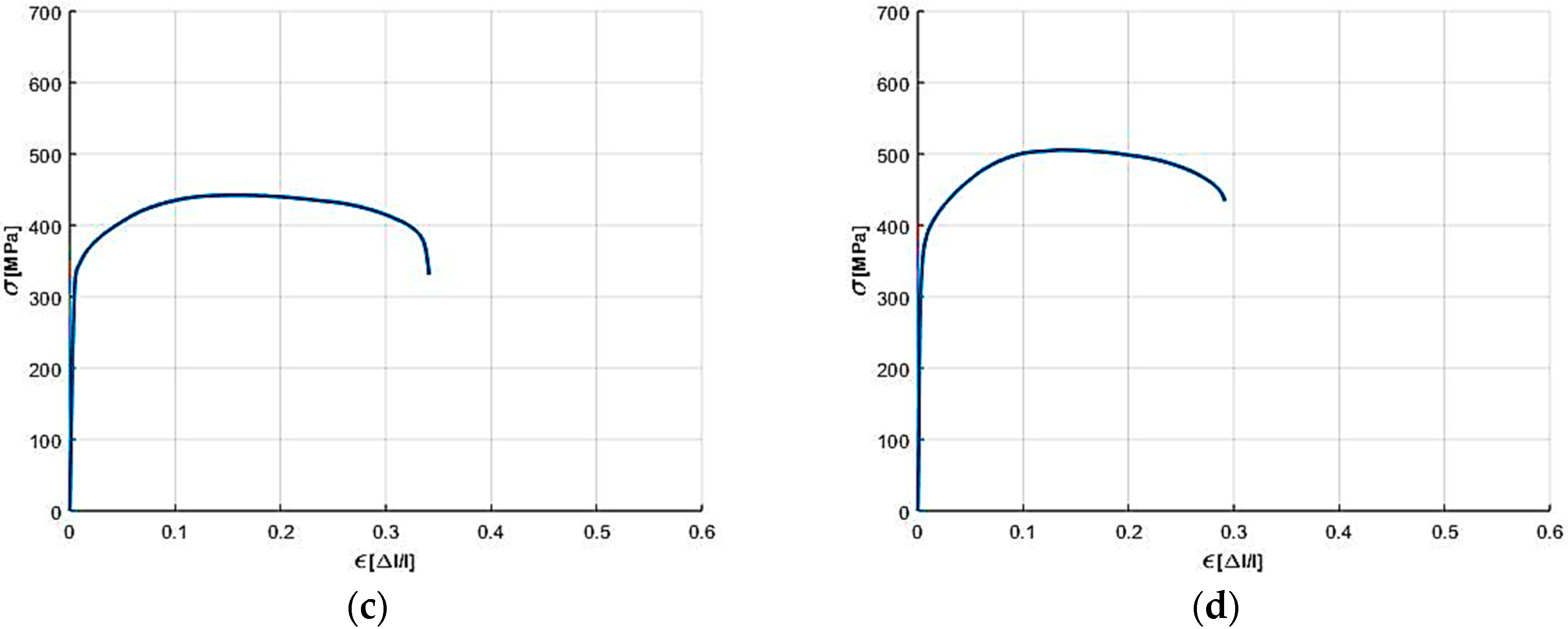
The mean experimental stress–strain curves at room temperature for the considered materials are reported in Figure 1.

All of the considered steels were characterized by a sigma–epsilon curve calculated according to the specification for the tensile tests for pipes (UNI EN ISO 6892), for each combination of diameter and thickness.

2.2. Model

A commercial software package integrated with its own solver, commonly used by automotive engineers, was adopted for the numerical calculations. Inside the software framework [16,17] the Hill 48' yield function was adopted, ideal for small-sized tubular geometries [11], as a constitutive equation for stainless steels’ behavior.

The following parameters are taken into account in order to simulate the bending process:

• Bending radius
• Bending angle
• Rotational speed

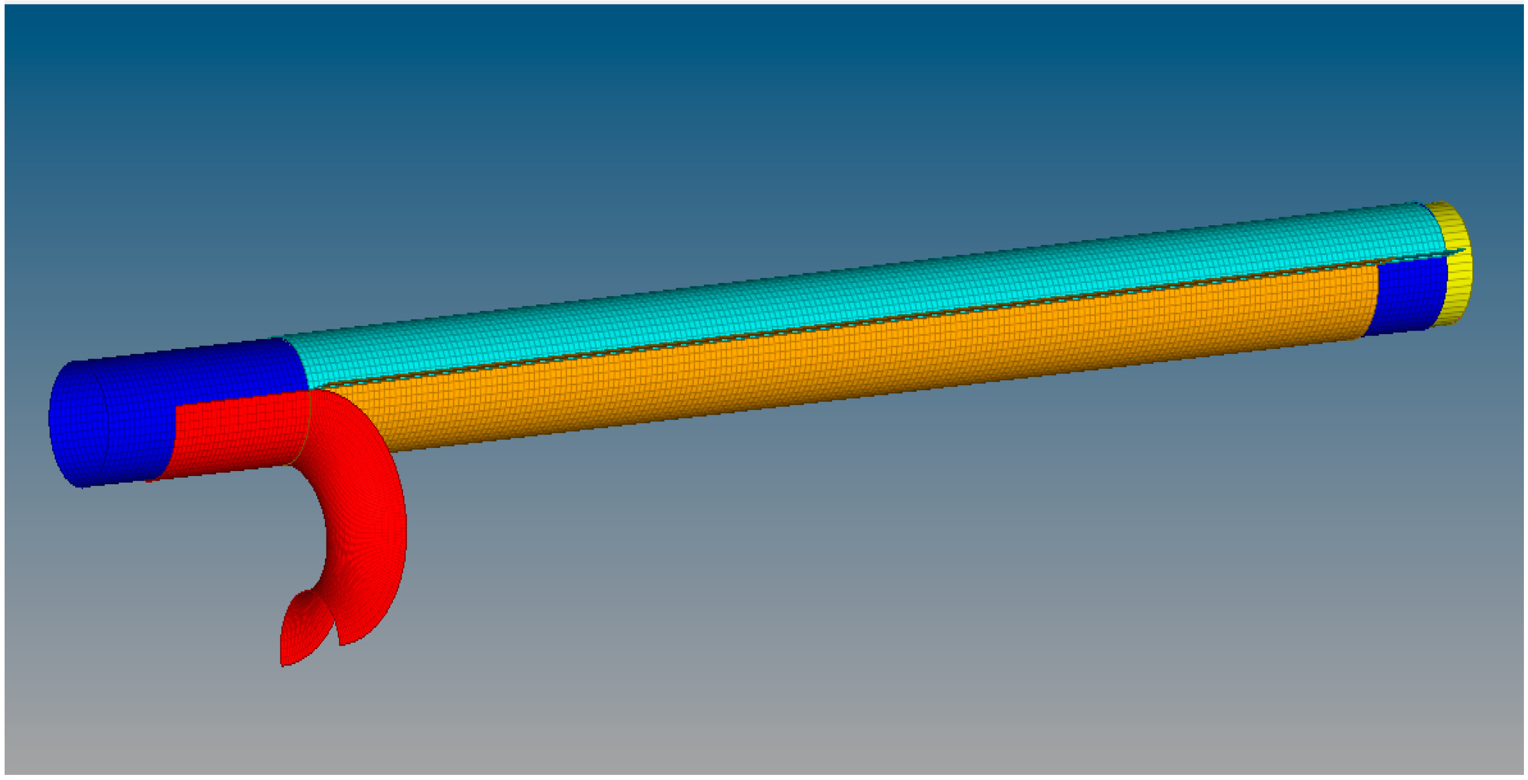
Based on the above assumptions/inputs, it is possible to simulate the pipe bending behavior. A typical model for such an approach is as reported in Figure 2.

2.3. Methodology of Analysis

The analysis of the simulation outputs is carried out through mappings of the values calculated by the solver (such as internal stress, thinning, and deformation). Specifically, the stress analyzed is an equivalent stress calculated by the solver on the basis of the Hill criterion, which is a mathematical form optimized for the Finite Element Analysis (FEA) and developed starting from the Von Mises criterion. In order to analyze the influence that the parameters have on the final process and on the feasibility, the maximum values obtained on the mappings will be considered in order to consider the critical points on the geometry.

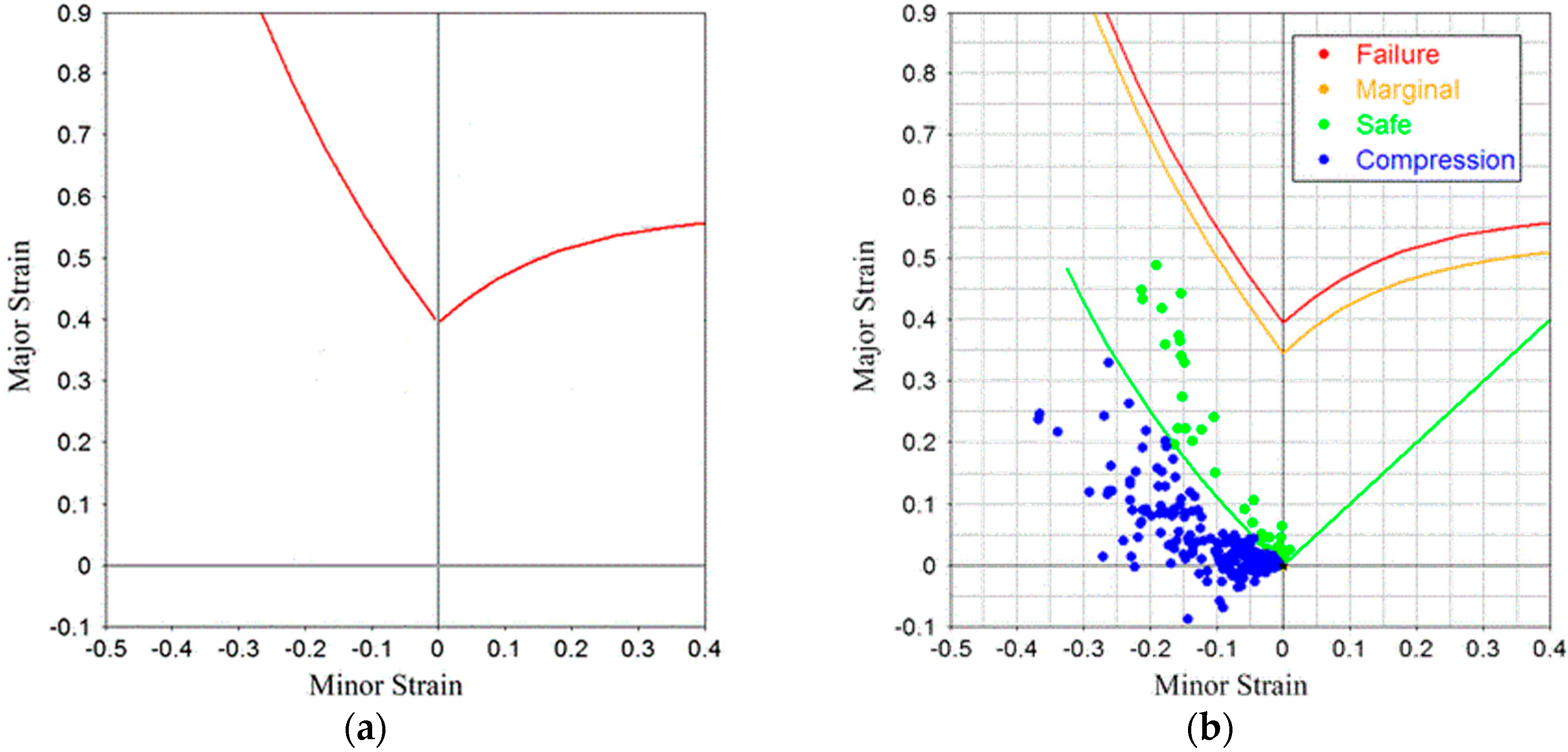
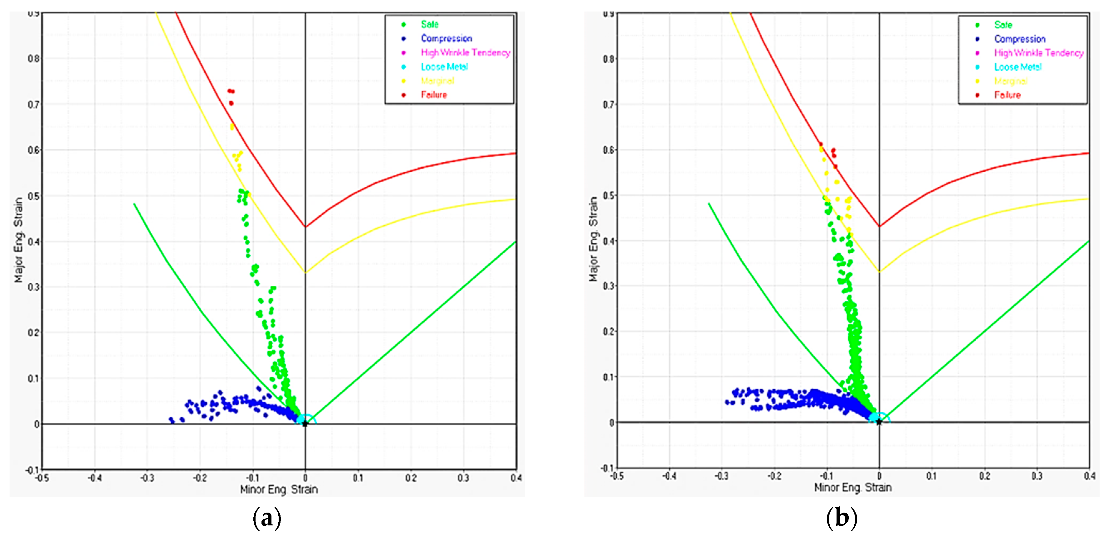
Usually, however, above all in the industrial field, a diagram defined as formability limit diagram (FLD) is used to describe the deformation paths along the whole sample. This diagram, as shown in the Figure 3, contains the formability limit curve (FLC), showing the maximum capacity of a material to be deformed, calculated by carrying out repeated Nakazima tests. The strains obtained from this test are measured with a conventional grid method, creating a pattern of circles on the surface of the specimen, which are deformed during the process obtaining ellipses. On these ellipses, the strains on the minor and major dimensions are measured, identifying the deformation state points of the material on the FLD diagram.

3. Results and Discussion

The influence of the different input parameters are reported below.

3.1. Diameter Influence

The typical ratio between the curvature radius and the pipe diameter (R/D) for industrial application is in the range between 1.0 and 1.5. Therefore, considering the various diameter cases, it was decided that R/D = 1 as a constant value, which aimed to consider cases that are actually representative of the real processes, and to have results, in terms of stress, that can be compared with each other.

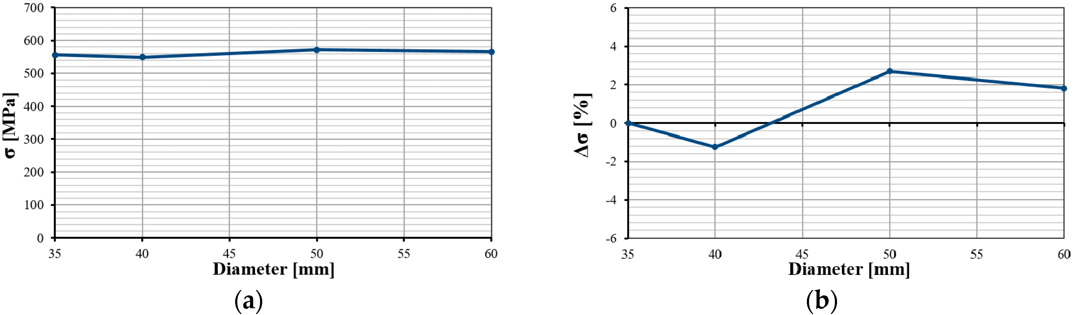
Figure 4 shows the stress mapping for smaller and larger diameters, while Figure 5 shows the stress reached for each diameter.

The results show that by varying the diameter and always keeping the ratio R/D = 1, a variation of the maximum stresses in a range between −2% and 3% is found; such an effect can be considered negligible. Furthermore, it is also evident that the distribution of the internal stresses is not particularly modified with the increase in diameter.

Additionally, in order to evaluate the deformation capacity of the various samples, the FLD diagrams were compared, and Figure 6 shows the extreme cases of the analyzed range of stainless steel AISI 304 with a 35 and 60 mm diameter. Furthermore, from the FLD diagrams, it can be deduced that the deformation path of the various elements of the geometry are not particularly modified by this parameter.

3.2. Influence of Thickness

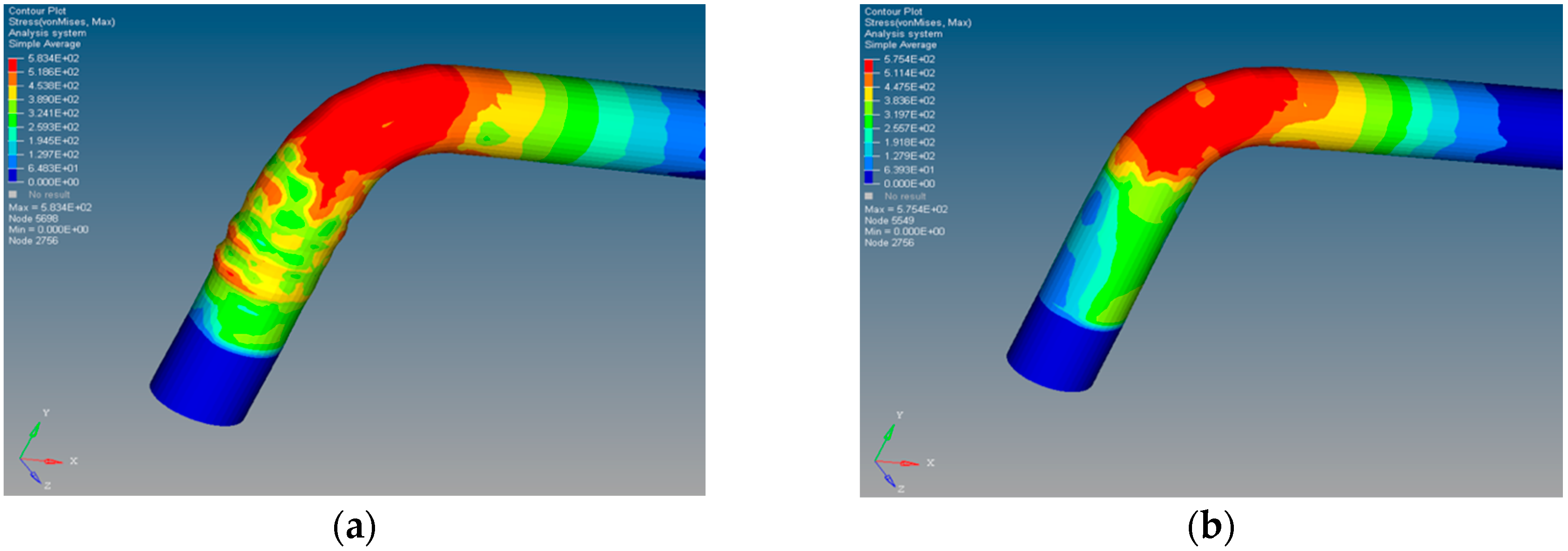
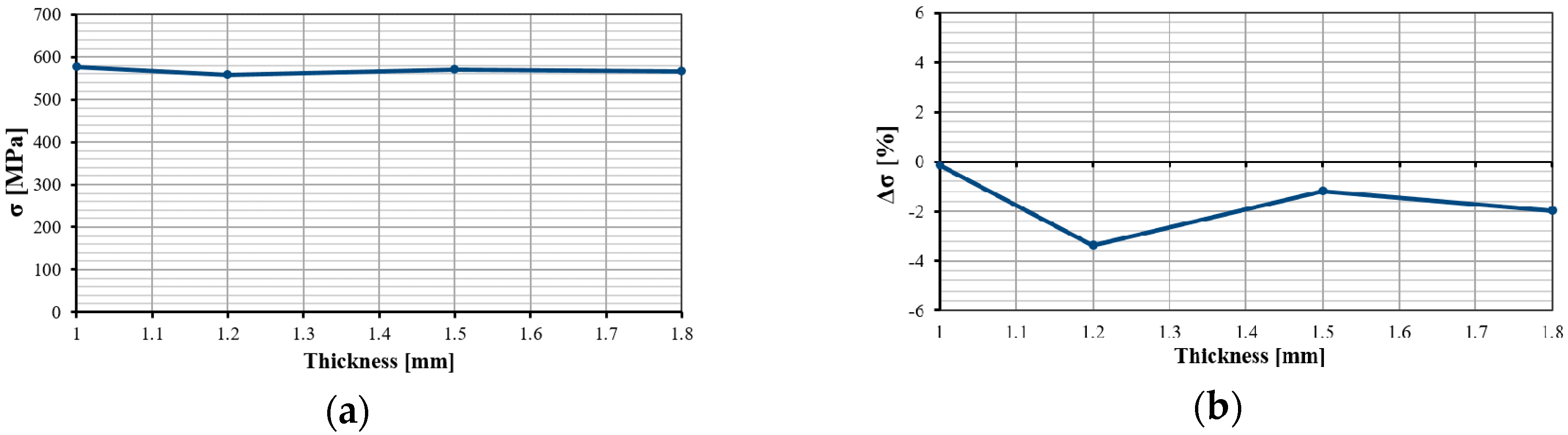
As for the study carried out for the diameter, the same cases have been analyzed, however varying the thickness of the tube and keeping all the other parameters constant and equal to the case studies of the diameter, such as R/D = 1. Figure 7 shows stress mapping for smaller and larger thickness and in Figure 8 their distribution as before.

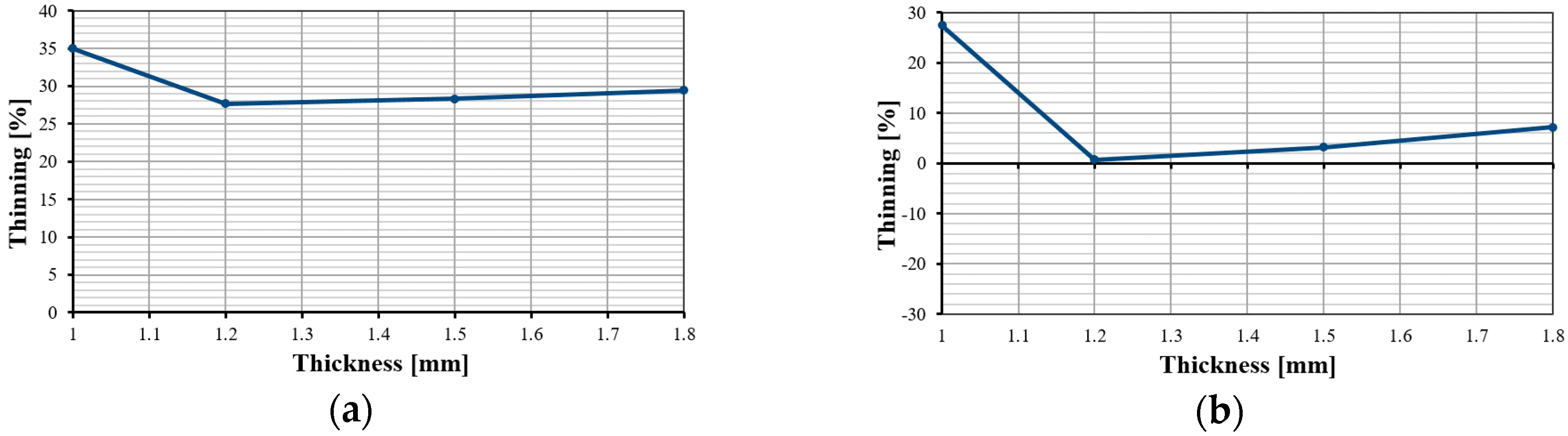
While from the graphs of the maximum stresses there is not a substantial difference, except for an oscillating decreasing trend, depending on the thickness, it is noticed in the images of the distributions that there is a processing failure for the thickness of 1 mm. Therefore, to deepen the analysis, the thinning caused by the working on the tube geometry was considered, as shown in Figure 9. From these graphs, it is more evident how the initial thickness of the geometry has a strong impact on the success of the bending process. In fact, we can see, first of all, the decreasing trend, even if it does not appear to be monotonic, confirming what was supposed before, but above all, the variation that this parameter involves, having a percentage difference of about 30% in the final thickness of the most stressed area.

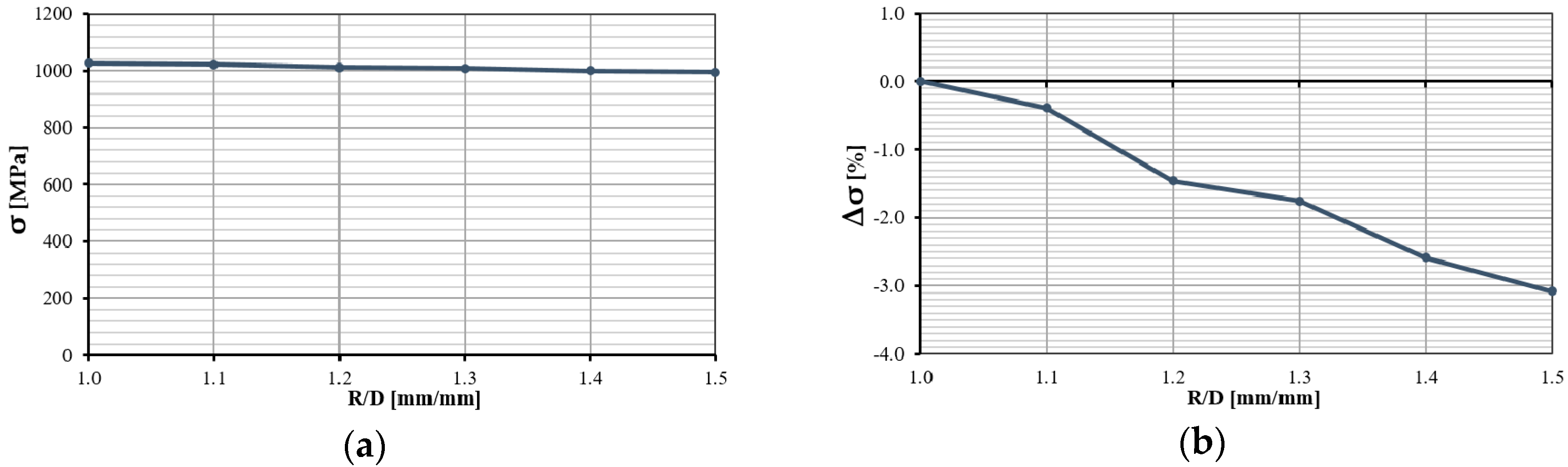
3.3. Influence of the R/D Ratio

The R/D ratio, defined as the radius of curvature/diameter, as previously mentioned, is a parameter not present within the simulation model, but is widely used in industrial applications. It is primary used as a feasibility index for processing and is generally between 1.0 and 1.5 in standard conditions. Already, in the case R/D = 1 (radius of curvature equal to diameter), the tube undergoes a considerable stress, and for lower values, there is a breakage of the piece in almost all of the cases with the standard processing conditions; therefore, in this case, particular precautions are necessary. For this reason, no cases of R/D < 1 have been studied and values of R/D greater than 1.5 are instead used for larger pipes, ducts, or special cases that are not present in the application fields of the pipes produced by the company.

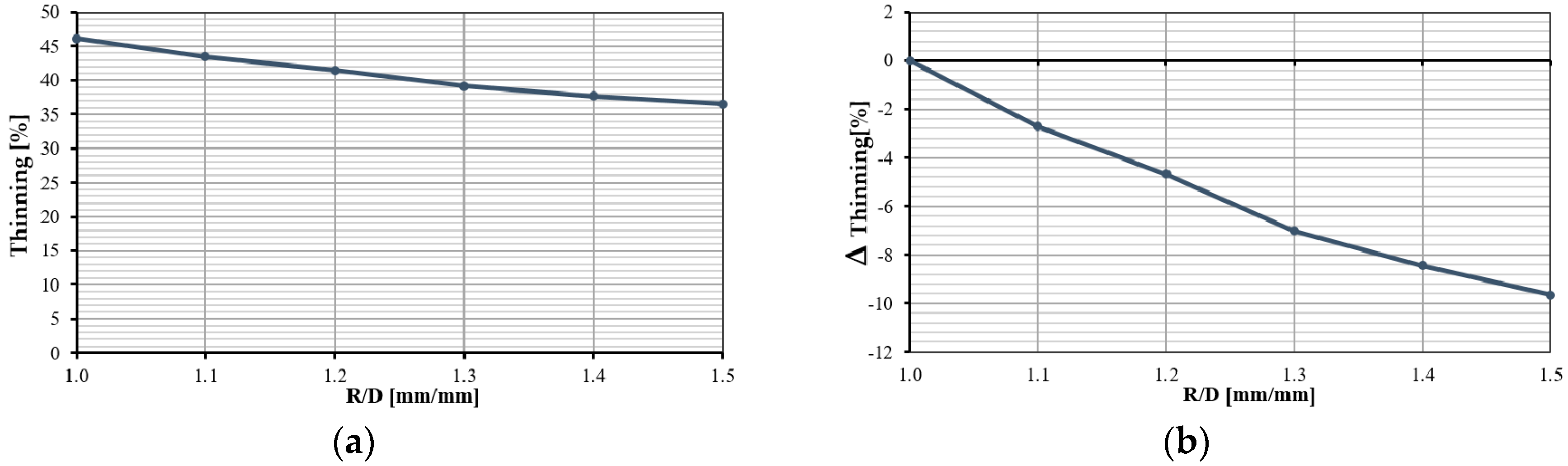
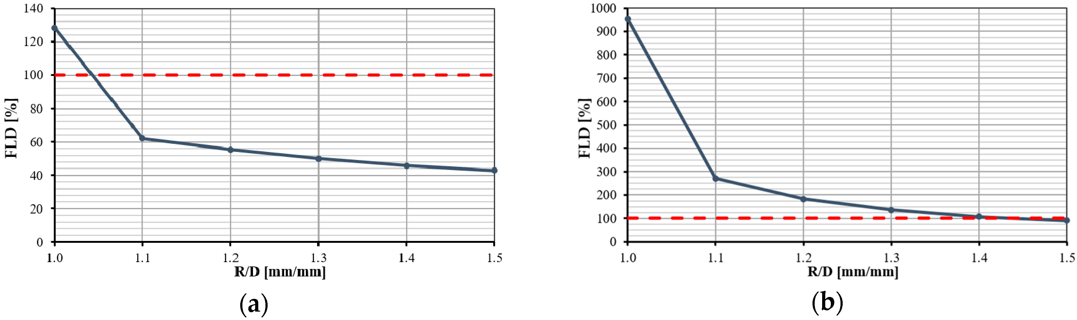
Then, by performing the simulations (with a constant diameter and then varying the radius of curvature) and analyzing the results, we see how, in Figure 10, the stresses achieved do not vary significantly by increasing the R/D ratio, but, as also seen for the other case studies, the maximum internal stress results are not sufficient to correctly describe the influence of the parameter. In fact, as can be seen in Figure 11, as the R/D ratio increases, the maximum thinning obtained decreases, therefore, although one would expect a decrease in stress, an increase in the ratio (obtained by increasing the radius of curvature or decreasing the diameter) causes minor forces in the tube and, at the same time, a minor thinning (as seen in Figure 11), thus significantly attenuating their decrease. It is also useful to observe the FLD diagrams in order to be able to make further considerations. Therefore, in Figure 12, it can be observed that both for the austenitic and ferritic steels, the increase in the R/D ratio leads to an increase in the feasibility of bending, which is very important, especially for AISI 409, because of its low plastic deformability compared with other families of the stainless steels considered.

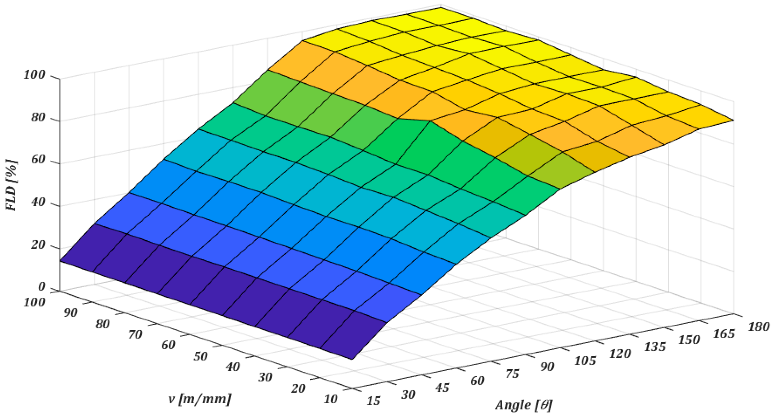
3.4. Influence of Velocity Based on the Bend Angle

In this case, for the study of velocity, the effect of its variation for each bend angle, which is generally set during the common forming processes (specifically, angles between 30° and 90°), has been analyzed. Furthermore, angles of more than 90° have been considered for completeness, and in order to verify the trend that involves the variation of speed, up to a maximum of 180°.

So, it can be initially observed, in Figure 13, how the percentage reached of the formability limit is mapped for each combination of the speed and angle.

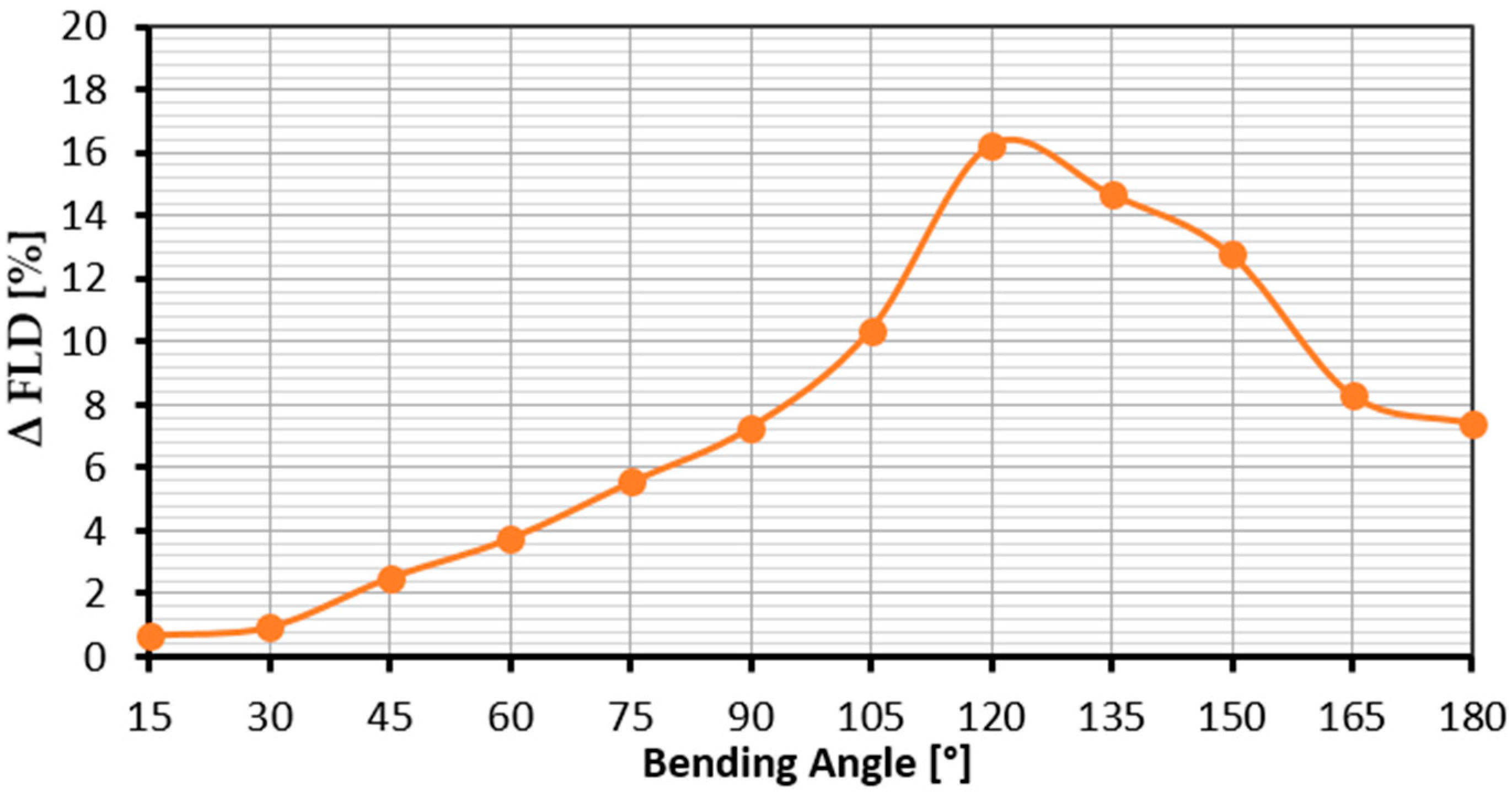
Moreover, in order to more advantageously evaluate the influence of the speed variation, it was decided to report the variation between percentage obtained for minimum and maximum speed of each considered angle, according to the Equation 1, in a graph (Figure 14), thus obtaining a graph purely from the variation itself.

ΔFLD = FLD_v-max − FLD_v-min

(1)

Therefore, as can be observed from Figure 14, it is noted that for the region of angles between 30° and 90°, which is the range of interest for common industrial processes, the influence of speed variation assumes an approximate linear trend against the bend angle. Instead, considering the whole range of study, it can be observed that the variation tends to reach a maximum at about 120° of bending, then returning to decrease with the increasing angle. The motivations that lead to this particular behavior can be studied in more detail, but currently, we can hypothesize, also observing Figure 15, that this is due to the concentration of stress that is more localized in the first 90° of bending, where the machine actually deforms the tube continuously and applies the forces involved in forming.

3.5. Experimental Validation

3.5.1. Validation Methods

In order to be able to consider these results correctly, it is necessary to validate the simulation model by comparing it with the corresponding real case in the same conditions. Six samples of tubes, for each of the following stainless steels families, were then examined:

• AISI 304
• AISI 316
• AISI 409
• AISI 441

All of the samples have the same dimensions corresponding to the simulation performed, a diameter 60 mm and thickness 1.2 mm. For each steel family, one of the six samples, for each group, were used to obtain, through tensile tests as before, the specific stress–strain curves, in order to eliminate the uncertainty due to the use of a mean curve. Both the tests and the simulations have been carried out with the settings, the rotational velocity and bending radius, that are actually used by the industries for the typical finishing process.

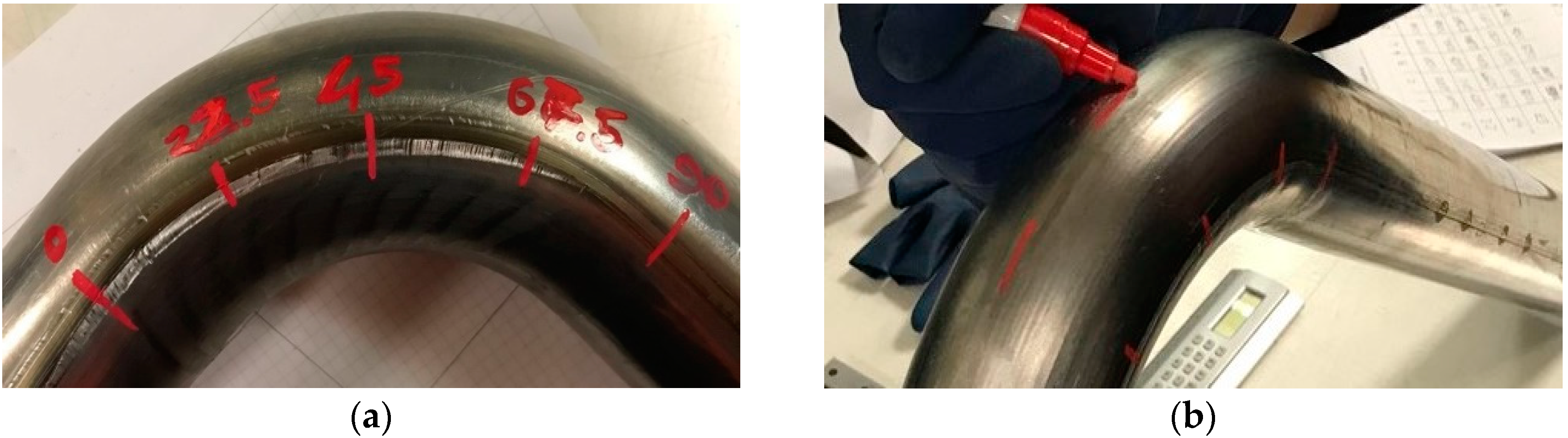
For the comparison, we decided to measure both of the thicknesses reached during the bend along the backbone at specific angles, as shown in Figure 16.

3.5.2. Validation Results

The values of the thicknesses were measured for each marked angle, and the average has been calculated. The values obtained are shown in

Table 1. Thickness for the AISI 304 samples.

Measurement Angle	Sample n° 1	Sample n° 2	Sample n° 3	Sample n° 4	Sample n° 5	Sample n° 6	Mean Value
0°	1.169	1.200	1.180	1.124	1.250	1.235	1.108
22.5°	1.003	1.019	1.026	1.023	1.023	1.101	1.037
45°	0.982	0.993	1.002	1.058	1.157	1.016	1.039
67.5°	1.086	1.016	1.050	1.029	1.166	1.052	1.042
90°	1.200	1.146	1.180	1.152	1.149	1.161	1.149

,

Table 2. Thickness for the AISI 316 samples.

Measurement Angle	Sample n° 1	Sample n° 2	Sample n° 3	Sample n° 4	Sample n° 5	Sample n° 6	Mean Value
0°	1.091	1.131	1.290	1.119	1.119	1.123	1.119
22.5°	1.023	1.010	1.028	1.014	1.048	1.032	1.026
45°	1.016	0.999	1.004	0.986	0.987	1.021	1.002
67.5°	1.028	1.015	1.021	1.030	1.071	1.017	1.030
90°	1.135	1.101	1.149	1.128	1.192	1.143	1.140

,

Table 3. Thickness for the AISI 409 samples.

Measurement Angle	Sample n° 1	Sample n° 2	Sample n° 3	Sample n° 4	Sample n° 5	Sample n° 6	Mean Value
0°	1.080	1.067	1.070	1.075	1.083	1.079	1.076
22.5°	0.959	0.961	0.950	0.963	0.942	0.962	0.956
45°	1.011	0.970	0.936	0.911	1.026	0.937	0.965
67.5°	0.987	0.971	0.968	0.990	1.010	0.989	0.986
90°	1.200	1.092	0.097	1.107	1.079	1.096	1.112

and

Table 4. Thickness for the AISI 441 samples.

Measurement Angle	Sample n° 1	Sample n° 2	Sample n° 3	Sample n° 4	Sample n° 5	Sample n° 6	Mean Value
0°	1.169	1.200	1.180	1.124	1.250	1.235	1.193
22.5°	1.003	1.019	1.026	1.023	1.123	1.101	1.049
45°	0.982	0.993	1.002	1.058	1.157	1.016	1.035
67.5°	1.086	1.016	1.050	1.029	1.166	1.052	1.067
90°	1.200	1.180	1.180	1.152	1.149	1.161	1.166

, in millimeters.

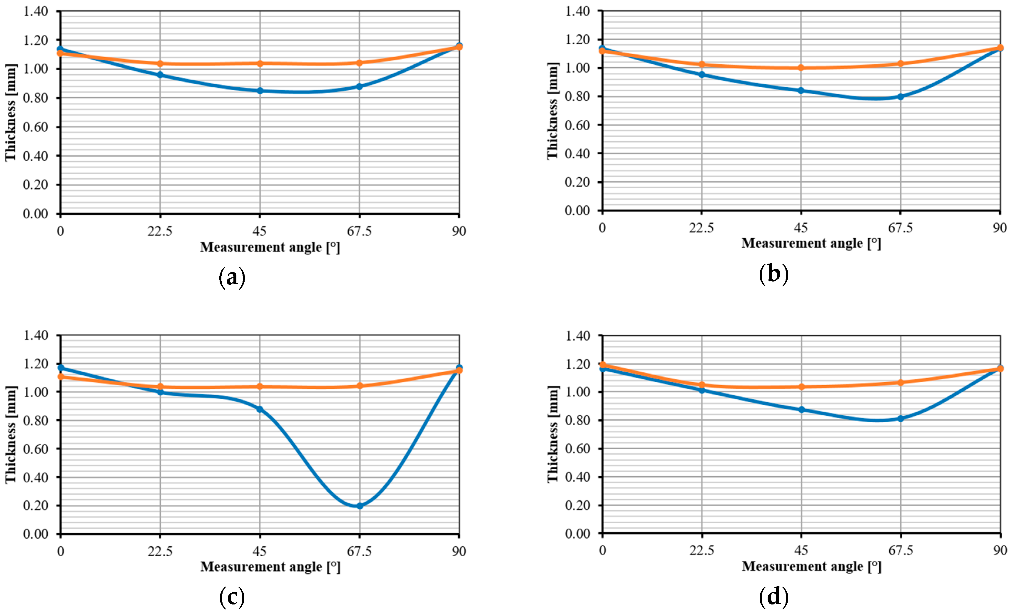
The same measures were extracted from the simulation result in the same points. The thickness variation and the percentage variation of the simulation, with respect to the real case, were then calculated to have a first feedback on the goodness of the predictive model adopted.

Table 5. Thickness for the AISI 304 samples.

Measurement Angle	Simulation Thickness [mm]	Sample mean Thickness [mm]	Δ Thickness [mm]	Percentage Variation [%]
0°	1.138	1.108	0.031	2.80
22.5°	0.958	1.037	−0.079	−7.62
45°	0.850	1.039	−0.188	−18.10
67.5°	0.880	1.042	−0.162	−15.55
90°	1.160	1.149	0.010	0.87

,

Table 6. Thickness for the AISI 316 samples.

Measurement Angle	Simulation Thickness [mm]	Sample mean Thickness [mm]	Δ Thickness [mm]	Percentage Variation [%]
0°	1.135	1.118	0.007	0.62
22.5°	0.952	1.025	−0.073	−7.12
45°	0.840	1.002	−0.160	−16
67.5°	0.800	1.030	−0.230	−22.3
90°	1.135	1.140	−0.005	−0.43

,

Table 7. Thickness for the AISI 409 samples.

Measurement Angle	Simulation Thickness [mm]	Sample Mean Thickness [mm]	Δ Thickness [mm]	Percentage Variation [%]
0°	1.170	1.076	0.094	8.7
22.5°	1.000	0.956	0.044	4.6
45°	0.880	0.965	−0.085	−8.8
67.5°	0.200	0.986	−0.786	−79.7
90°	1.170	1.112	0.058	5.2

and

Table 8. Thickness for the AISI 441 samples.

Measurement Angle	Simulation Thickness [mm]	Sample Mean Thickness [mm]	Δ Thickness [mm]	Percentage Variation [%]
0°	1.166	1.193	−0.027	−2.26
22.5°	1.013	1.049	−0.036	−3.43
45°	0.874	1.035	−0.161	−15.56
67.5°	0.814	1.067	−0.253	−23.71
90°	1.171	1.166	0.005	0.42

show the calculated data and Figure 17 shows the trends of the four families of stainless steels considered.

The above figures show that the simulation results are in agreement with the real case. It is noted that the major deviation occurs in all four of the cases for 67.5° of measurement, and a maximum deviation of −79.7% for AISI 409 and 18–24% for the other stainless steels is reached. As a matter of fact, it is important to note that there is a huge difference between the two cases, specifically for the 67.5° of AISI 409 ferritic stainless steel, but this is due to the fact that for this particular case there is a localized break near the considered angle on the simulation results, and furthermore, the maximum variation for AISI 304, 316 and 441 corresponds to a value in the range of 0.16–0.25 mm. The difference between realty and simulation, for both the failure of AISI 409 and for the general variation of the other three stainless steels families, is due to the presence of an additional support element present in most of the bending machines, called a ‘booster’, which was not present in the simulation model. Its function is precisely that of pushing the tube during bending, in order to avoid the deformations or failure caused by the friction between the element and the machine or by the concentration of stresses. Its action also affects the distribution of the thinning, caused by the deformation, in fact, of the tube being pushed by the booster, which will have more evenly distributed the stresses on itself, and consequently, the deformations and the thinning will take place on a wider area and will not lead to failure of the piece.

4. Conclusions

In this paper, the bending process of stainless steel pipes has been studied. The experimental investigations coupled with simulations highlighted the importance of each parameter, both operational and geometric, on the final results.

In particular, it has been observed that the pipe diameter does not prove to be a decisive parameter for the success of the working process, while the pipe thickness appears to be a determinant factor for failure and/or unwanted deformation of the formed piece. The R ratio is extremely important; in fact, its variation within the standard range (between 1.0 and 1.5) identified the transition between the failure and success of the operation, both for the AISI 304 austenitic stainless steel and for AISI 409 ferritic stainless steel, of which for the latter led to a 90% increase in feasibility.

The combined study of the rotational speed and bending angle allowed us to define a trend of influence for these operating parameters, showing how there is a linear increase in the influence of the speed in the range between 30° and 90° of bending, while for the angles higher than around 120°, this tendency is reversed.

The overall experimental validation showed a deviation of the model from the reality, between an overestimation of 8% to an underestimation of 20%, with the maximum displacement generally located on the back of the bending, probably due to the presence in the experimental tests of an additional element support of the machinery, called a booster, which was not contemplated in the simulation model. Furthermore, the maximum deviation recorded corresponds to a deviation in thickness between the two cases in the order of 10⁻² mm, thus resulting in a good starting point for the refinement and optimization of the final model.

Moreover, thanks to this analysis and the preliminary experimental tests, the FEM simulation has proved to be a useful tool in order to predict the industrial deformation processes, where there are currently no means to characterize the processes generally carried out on these components, but only of the empirical methods to define its overall feasibility.

References

- Marshall, P. Austenitic Stainless Steels; Springer: Heidelberg, Germany, 1984; ISBN 978-0-85334-277-9. [Google Scholar]
- Di Schino, A.; Barteri, M.; Kenny, J.M. Fatigue behavior of a high nitrogen austenitic stainless steel as a fuction of its grain size. J. Mater. Sci. Lett. 2003, 22, 1511–1513. [Google Scholar] [CrossRef]
- Di Schino, A.; Kenny, J.M.; Salvatori, I.; Abbruzzese, G. Modelling recrystallization and grain growth in low nickel austenitic stainless steels. J. Mater. Sci. 2001, 36, 593–601. [Google Scholar] [CrossRef]
- Di Schino, A.; Kenny, J.M.; Barteri, M. High temperature resistance of high nitrogen low nickel austenitic stainless steels. J. Mater. Sci. Lett. 2003, 22, 691–693. [Google Scholar] [CrossRef]
- Corradi, M.; Di Schino, A.; Borri, A.; Rufini, R. A review of the use of stainless steel for masonry repair and reinforcement. Constr. Build. Mater. 2018, 181, 335–346. [Google Scholar] [CrossRef]
- Badoo, N.R. Stainless steel in construction: A review of research, applications, challenges and opportunities. J. Constr. Steel Res. 2008, 64, 1199–1206. [Google Scholar] [CrossRef]
- Lo, K.H.; Shek, C.H.; Lai, J.K.L. Recent development in stainless steels. Mater. Sci. Eng. R Rep. 2009, 65, 39–104. [Google Scholar] [CrossRef]
- Gardner, L. The use of stainless steel in structures. Prog. Struct. Eng. Mater. 2005, 7, 45–52. [Google Scholar] [CrossRef]
- Bong, H.J.; Barlat, F.; Lee, M.G.; Ahn, D.C. The forming limit diagram of ferritic stainless steel sheets: Experiments and modeling. Int. J. Mech. Sci. 2012, 64, 1–10. [Google Scholar] [CrossRef]
- Yang, T.B.; Yu, Z.Q.; Xu, C.B.; Li, S.H. Numerical analysis for forming limit of welded tube in hydroforming. J. Shanghai Jiaotong Univ. 2011, 45, 6–10. [Google Scholar]
- Zhang, H.; Liu, Y. The inverse parameter identification of Hill’48 yield function for small-sized tube combining response surface methodology and three-point bending. J. Mater. Res. 2017, 32, 2343–2351. [Google Scholar] [CrossRef]
- Zhan, M.; Guo, K.; Yang, H. Advances and trends in plastic forming technologies for welded tubes. Chin. J. Aeronaut. 2016, 29, 305–315. [Google Scholar] [CrossRef]
- Giannella, V.; Fellinger, J.; Perrella, M.; Citarella, R. Fatigue life assessment in lateral support element of a magnet for nuclear fusion experiment “Wendelstein 7-X”. Eng. Fract. Mech. 2017, 178, 243–257. [Google Scholar] [CrossRef] [Green Version]
- Citarella, R.; Giannella, V.; Lepore, M.A.; Fellinger, J. FEM-DBEM approach to analyse crack scenarios in a baffle cooling pipe undergoing heat flux from the plasma. AIMS Mater. Sci. 2017, 4, 391–412. [Google Scholar] [CrossRef]
- Khalfallah, A.; Oliveira, M.C.; Alves, J.L.; Zribi, T.; Belhadjsalah, H.; Menezes, L.F. Mechanical characterization and constitutive parameter identification of anisotropic tubular materials for hydroforming applications. Int. J. Mech. Sci. 2015, 104, 91–103. [Google Scholar] [CrossRef]
- Dama, K.K.; Snirivasulu, S.; Swaroop, D. Design for crashworthiness of an automotive sub-system using cae techniques. Int. J. Mech. Eng. Technol. 2018, 9, 21–27. [Google Scholar]
- Cao, F.; Li, J.; Cui, M. Analysis of frame structure of medium and small truck crane. AIP Conf. Proc. 2018, 1944. [Google Scholar] [CrossRef]
Figure 1.
Examples of experimental stress–strain curves for the considered materials, obtained from tensile tests at room temperature on the pipes for the following grades of stainless steel: (a) AISI 304; (b) AISI 316; (c) AISI 409; and (d) AISI 441.
Figure 2.
Geometry and working parts of the machinery simulated inside the software.
Figure 3.
Typical shape of the formability limit curve (a); example of Nakazima’s experimental test results on the formability limit diagram (FLD) with deformation state points for an AISI 304 stainless steel sheet (b).
Figure 4.
Equivalent stress mapping for diameters of 35 mm (a) and 60 mm (b) for AISI 304, 1.5 mm thickness.
Figure 5.
Trend of maximum equivalent stress according to the diameter for AISI 304, 1.5 mm thickness (a); percent variation of maximum equivalent stress according to the diameter for AISI 304, 1.5 mm thickness (b).
Figure 6.
FLD diagrams of 35 mm (a) and 60 mm (b) for AISI 304, 1.5 mm thickness.
Figure 7.
Equivalent stress mapping for a thickness of 1 mm (a) and 1.8 mm (b) for AISI 304, 50 mm diameter.
Figure 8.
The trend of maximum equivalent stress according to thickness for AISI 304, 50 mm diameter (a); percent variation of maximum equivalent stress according to the thickness for AISI 304, 50 mm diameter (b).
Figure 9.
Trend of maximum thinning according to thickness for AISI 304, 50 mm diameter (a); percent variation of maximum thinning according to thickness for AISI 304, 50 mm diameter (b).
Figure 10.
Trend of maximum equivalent stress according to the curvature radius and the pipe diameter (R/D) ratio for AISI 304 (a); percent variation of maximum equivalent stress according to the R/D ratio for AISI 304 (b).
Figure 11.
Trend of maximum thinning according to the R/D ratio for AISI 304 (a); percent variation of maximum thinning according to the R/D ratio for AISI 304 (b).
Figure 12.
Percentage reached of the formability limit (red dashed line) according to the R/D ratio for AISI 304 (a) and AISI 409 (b).
Figure 13.
Percentage reached of the formability limit for every combination of speed and angle for AISI 304.
Figure 14.
Percentage of formability limit variation in the minimum–maximum speed range as a function of the bending angle for AISI 304 steel.
Figure 15.
Equivalent stress mapping for bending angle of 90° (a); 120° (b); 150° (c); and 180° (d), at 2.7 rad/s for AISI 304.
Figure 16.
Thicknesses measuring grid on the backbone (a,b).
Figure 17.
Thickness trend for the simulation case (blue) and real case (orange) for AISI 304 (a); AISI 316 (b); AISI 409 (c); and AISI 441 (d).