Numerical Prediction of Forming Car Body Parts with Emphasis on Springback


1
Department of Mechanical Technology and Materials, Faculty of Mechanical Engineering, Technical University of Košice, Mäsiarska 74, 040 01 Košice, Slovakia
2
Department of Computer Support of Technology, Faculty of Mechanical Engineering, Technical University of Košice, Mäsiarska 74, 040 01 Košice, Slovakia
*
Author to whom correspondence should be addressed.
Metals 2018, 8(6), 435; https://doi.org/10.3390/met8060435
Submission received: 27 April 2018
/
Revised: 31 May 2018
/
Accepted: 6 June 2018
/
Published: 8 June 2018
(This article belongs to the Special Issue Modelling and Simulation of Sheet Metal Forming Processes)
Abstract
:Numerical simulation is an important tool which can be used for designing parts and production processes. Springback prediction, with the use of numerical simulation, is essential for the reduction of tool try-outs through the design of the forming tools with die compensation, therefore, increasing the dimensional accuracy of stamped parts and reducing manufacturing costs. In this work, numerical simulation was used for performing the springback analysis of car body stamping made of aluminium alloy AA6451-T4. The finite element analysis (FEM) based software PAM-STAMP 2G was used for performing the forming and springback simulations. These predictions were conducted with various combinations of material models to achieve accurate springback prediction results. Six types of yield functions (Barlat89, Barlat2000, Vegter-Lite, Hill90, Hill48 isotropic, and Hill48 orthotropic) were used in combination with the Voce hardening model. Springback analysis was conducted in three sections of the formed part; the numerical results were compared with the experimental values. It was found that the combinations of Barlat’s yield functions and the Voce hardening law were most accurate in terms of springback prediction. Additionally, it was found that the phenomena that were investigated, which are required for the determination of the kinematic hardening model, such as the change of Young’s modulus E, the transient behaviour, work-hardening stagnation, and permanent softening, were not observed in the aluminium alloy studied.
1. Introduction
Automobile manufacturers have started to use new types of high strength steels (HSS, AHSS, and UHSS) at the end of the last century, with the aim of increasing the passive safety of vehicles and to reduce vehicle weight to decrease fuel consumption [1,2,3]. However, these types of steels have a lower formability in comparison with steels used for deep drawing. The main reason for this is the higher values of the yield strength and lower ductility of high strength steels [2]. In addition, aluminium alloys are now widely used in the automotive industry due to advantages, including the low density, high specific strength, good corrosion resistance, exceptional specific stiffness, and so forth [1]. The implementation of aluminium alloys in car body production can reduce fuel consumption and emissions [4]. Both high strength steels and aluminium alloys are more prone to wrinkling and springback than mild steels [1,5].
Springback in the present refers to a change of shape which is elastically driven. Springback occurs following a sheet-forming operation when the forming loads are removed from the workpiece—sheet metal blank. It is usually unwanted, causing problems in the next forming operations, in assembly, and in the final product. These problems usually degrade the accuracy, appearance, and quality of the products being manufactured [2,3,6]. The most common counter measurement against the springback of car body parts is to design a forming tool with anticipation of springback, thus compensating springback by die design. However, the amount of compensation is a difficult question even for skilled tool designers. In practice, this compensation of die is still sometimes done by the “trial and error” method. This method can be replaced by FEA (finite element analysis)—numerical simulation. With the use of FEA, it is possible to achieve a more accurate prediction of springback [6,7,8]. There are other counter measurements against springback, for example, the stiffening of pressings (use of beads or embossing), crash forming with pressure pads, the use of variable blank holder force, and so forth [7].
In general, two types of methods are used for springback prediction—finite element analysis and the analytical model. For example, the analytical model for springback prediction of aluminium alloys can be found in the work by Gau and Kinzel [9]. Analytical methods usually use simplified models of real processes. Thus, analytical models are usually not as accurate in predicting springback as numerical simulations and their use is limited, especially for stampings with complex geometry [10]. The finite element method (FEM) is a well-known tool for the prediction and analysis of sheet metal deformation. Springback prediction with the use of numerical simulation is not limited by the geometrical complexity of the stamped part like in the case of the analytical model. However, the numerical simulation of springback is more sensitive to the accuracy of the input data than the analytical method. Thus, it is very important to choose the correct input and numerical parameters in the FEA analysis of springback [11].
Numerical parameters involve the through-thickness integration scheme (which can be implicit, explicit, or a combination of both), the number of integration points, the used elements (type, size, and count), and so forth. Trzepiecinski and Lemu [12] studied the effect of a number of integration points and integration rules on the springback amount. Their results indicate that at least 5 integration points must be used to achieve accurate springback prediction. The input parameters involve geometry (sheet thickness, tool and sheet dimensions, and so forth), process conditions (type of forming method, tribology, forming forces, forming temperature and speed, and so forth), and material characteristics (Young’s modulus, yield strength, hardening behaviour, yield function, and so forth) [10,11]. Slota, Siser, and Dvorak [13] studied the effects of yield functions (isotropic and orthotropic) on the springback prediction accuracy of aluminium alloys. Their results showed that the orthotropic yield function is more accurate in predicting springback than the isotropic function. In addition, the effect of the die radius on springback was studied. They found out that the increase of the bending radius caused a higher springback of the bend materials. Seo et al. [14] conducted a study to evaluate the effect of constitutive equations on the springback prediction accuracy. They used two yield functions, Hill48 and Yld2000, in combination with the Yoshida-Uemori hardening model in the finite element (FE) simulation to predict the springback of the U-bend part and drawn T-shape part. Both parts were made of TRIP steel. They found out that it is essential to choose the right yield function to get an accurate prediction of springback. Mulidran et al. [15] conducted a numerical simulation of the drawing hat-shaped part made of the DP600 and DC04 steels with the use of two forming methods: drawing with a blank holder and crash forming with a pressure pad. They studied the effect of forming methods and the various process parameters on springback amount. Their results indicated that the higher blank holder and pad pressure have positive effects on reducing springback. Additionally, crash forming with a pressure pad showed lower springback in comparison with drawing with a blank holder. The work by Jung et al. [16] aimed at studying anisotropic hardening behaviour and the springback of AHSS steels. They proposed the modified isotropic-kinematic hardening model, which they used in the simulation of U-bending. Their model showed better results in the predicting springback in comparison with the isotropic hardening model.
The novelty of this work lies in findings which indicate that the isotropic hardening model is sufficient for predicting the springback of formed parts made of aluminium alloy. This model is simpler, and does not need cyclic shear tests. In addition, isotropic hardening models do not use as many parameters as kinematic hardening models. The accuracy of springback prediction with use of the isotropic hardening model was high. In addition, we found out that the phenomenon of the degradation of Young´s modulus is not present for aluminium alloys which are precipitation hardened, and that the degradation is not as significant as in AHSS steels (max. 2% degradation of Young´s modulus for aluminium alloys). Villuendas et al. [17] and Roca et al. [18] studied the effect of plastic deformation on the changes of Young´s modulus of metallic alloys. They reported that, in aluminium alloys, there were no appreciable changes in the E value. This conclusion is consistent with our findings. These changes are related to the dislocation density changes. However, even though the dislocation density is high, the values of parameter l (length of dislocations) are very low, due to the interaction between nanometric precipitates and dislocations in the aluminium alloys. The Mott model then shows that the change of Young´s modulus E is very small. Kinematic hardening models also take into account other phenomena, such as the transient behaviour, work-hardening stagnation, and the permanent softening. These phenomena were not observed in the material studied in this work.
These findings have a significant financial impact. For example, it is not necessary to conduct time-consuming tests on special (expensive) equipment, which are used to determine the parameters for kinematic hardening models.
In addition, the detailed analysis of a complex shaped part made of aluminium alloy with a significant thickness of 3 mm, mainly used in car production, was conducted. In most of the studied literature, the research was done on simply shaped parts.
In this research work, a FEM was used to predict the springback of a car body part made of aluminium alloy AA6451-T4. The finite element analysis (FEA) was conducted to investigate the influence of the used yield functions in the numerical simulation on springback prediction accuracy. Three sections were used for springback evaluation; in these sections, the thickness and part profile were measured and compared with the experimental results. The experimental results were given by the automobile manufacturer. Additionally, the computation times for the various yield functions were compared.
2. Materials and Methods
In the presented work, aluminium alloy AA6451-T4 with a thickness of 3.00 mm was used as the blank. Mechanical properties were measured by uniaxial and biaxial tensile tests. To obtain the required data for the FEM model, the specimens for the uniaxial tensile test were cut in three different orientations (0°, 45°, and 90° to the rolling direction). Specimens for the uniaxial tensile test were produced according to the EN 10002-1:2002-11 standards. Several specimens were tested for each orientation, and the average values of the basic mechanical properties (displayed in Table 1) were obtained by the formula
where X is the mechanical parameter, and the subscripts denote the orientation of the specimen with respect to the rolling direction of the sheet. The elastic mechanical properties of the aluminium alloy are shown in Table 2.
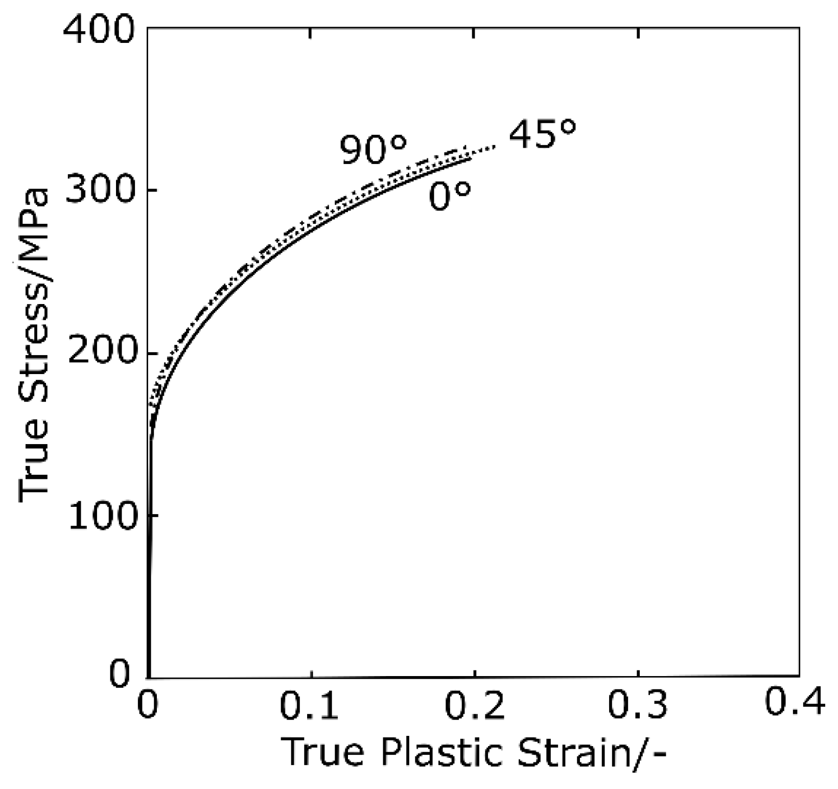
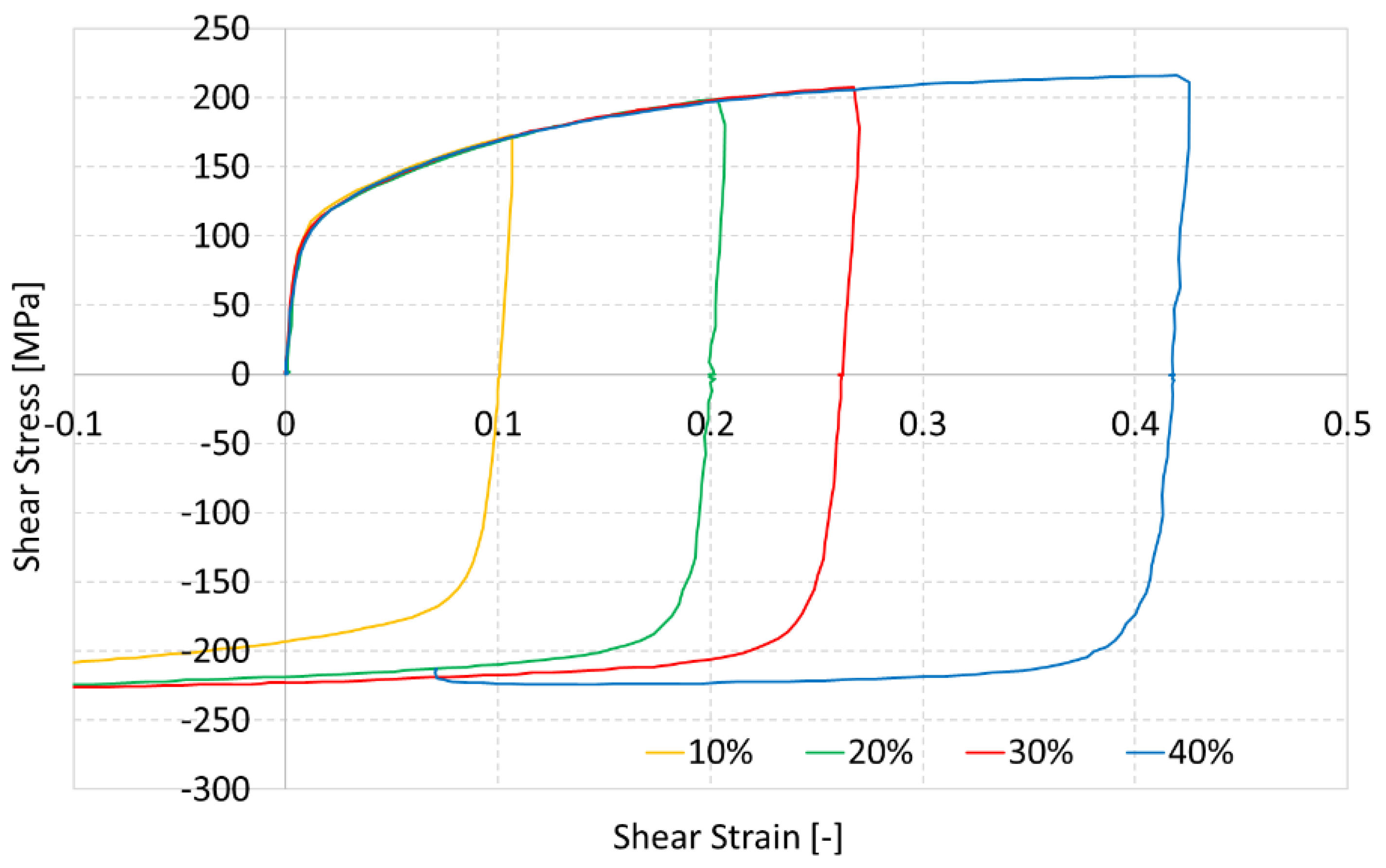
The true stress–strain curves obtained in three different orientations (0°, 45°, and 90° with respect to the rolling direction) are shown in Figure 1. The tension-compression test (Figure 2) was started by the tension load as the first part of the full cycle. After a specific crosshead stroke corresponding to a defined pre-strain level, the load was reversed to compression until it reached the crosshead displacement according to a given compression strain. Next, reloading in tension direction was introduced until the crosshead stroke was equal to that in the first tension. The investigated phenomena, such as the change of Young’s modulus E, transient behaviour, work-hardening stagnation, and permanent softening, were not observed in the material studied in this work, as we can see from Figure 2.
The equal biaxial tensile yield stress and the biaxial anisotropy rb are given in Table 3. The parameters obtained from this test are necessary to determine the advanced yield functions.
3. Numerical Model
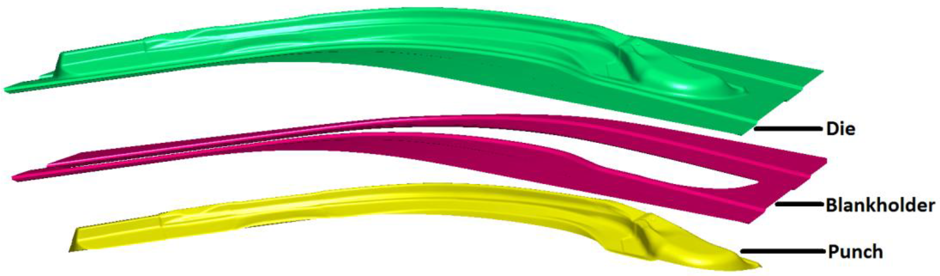
The springback computation was performed using the dynamic explicit code in the PAM-Stamp 2G software. The tool setup imported in the simulation software is shown in Figure 3. The tool consists of punch, blankholder, and die. The tool is aligned with the global z- axis without a plane of symmetry. The blank was positioned between the die and blankholder.
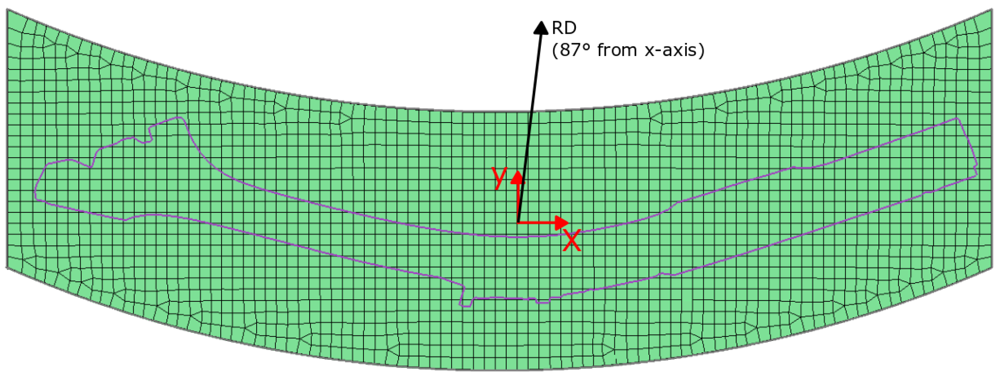
The blank was meshed by the quadrilateral shell elements which were 23 mm in size. The refinement level of the elements was set to 4 so that the smallest elements after refinement had a size of 2.875 mm. The number of integration points was set to 11, which is recommended for springback computation. The friction coefficient was set to 0.08, which responded to the grease lubrication. The initial meshed blank with a rolling direction is illustrated in Figure 4.
The obtained values of the mechanical properties were used as the basic input for the material model in the FEM simulation. The accuracy of the springback prediction for several yield functions was investigated by the FEM simulation. The yield function describes the material transition from the elastic state to the plastic state. It can be described as a function of the area that limits the elastic area of the multi-axis stress plane. In 1948, Hill introduced the concept of material anisotropy in yield functions. According to Hill’s plasticity conditions [20], in case of uniaxial load, a local thickness reduction occurs in a direction sensitive to the sample load. Hill assumed that the direction of the compression is in line with the direction of zero extension and, therefore, the deformation of the narrowed areas is only reflected as a reduction in thickness. This is assumed for the plane strain (σ1—major stress, σ2—minor stress, and σ3 = 0). If we assumed that the anisotropy axes are identical with the main guideline strain tensor (σx = σ1, σy = σ2, τxy = 0), it is possible to describe the Hill48 yield function by the formula
where σxx, σyy, and σzz are stresses in the RD (x), TD (y), and thickness (z) directions, respectively; σxy, σyz, and σzx are the shear stresses in xy, yz, and zx directions. Parameters F, G, H, and N are material parameters that describe the anisotropy of the material. If F = G = H = 1, and N = 3, the Hill48 function is reduced to the von Mises criterion, or as it is called in FEM code, the Hill48 isotropic criterion. A more common description is based on normal anisotropy in the 0°, 45°, and 90° directions to the rolling direction. Then, the material parameters F, G, H, and N can be described by
For orthotropic hardening law and the values of anisotropy under 1.0, the Hill90 yield function is more suitable. This function is considered to be more suitable for aluminium alloys, and it is based on a non-quadratic transition function. In order to construct this function, the values from the uniaxial tensile test are deficient. For a complete description of this function, the biaxial test data are also required. The function can be described as
where σ0 is uniaxial tensile stress in the rolling direction, σ90 is uniaxial tensile stress in the direction normal to the rolling direction, σb is the stress under the balanced biaxial stress, and the c, p, and q parameters are defined as follows [21]:
where R0 is the anisotropy value for the uniaxial tension in the rolling direction and R90 is the anisotropy value for the uniaxial tension in the in-plane direction, perpendicular to the rolling direction.
The Barlat’s material models describe the plastic behaviour of a material in a more detailed way than Hill’s functions, but the higher number of parameters increases the calculation time. The Barlat89 model needs three parameters for its complete formulation, by which it is possible to describe the plane strain behaviours. Those parameters are defined in Table 4. The formulation is the following:
where M is the exponent related to the crystallographic structure of the material, and k1 and k2 can be described as
where a, h, and p are the material model parameters.
A more precise function was presented by Barlat in 2003, called Barlat2000, where the linear transformation method was used. In the FEM software, this function is described by the eight parameters shown in Table 5. The formulation for this model is as follows:
where a is an exponent related to the crystallographic structure of the material and and are two isotropic functions described as follows [22]:
According to several works [23,24,25], the Vegter yield function should be more suitable for special steels and aluminium alloys due to its more convenient results. The Vegter criterion describes the yield locus more accurately from a series of physically tested points. According to Vegter, it is possible to establish the first quadrant of the yield function on the basis of the basic experimental measurement. To construct the ellipses, the Bezier interpolations between each point need to be performed. Every point requires three parameters to be defined, the main stresses σ1 and σ2, and the strain vector ρ = dε2/dε1. For a complete description of planar anisotropy, it is necessary to obtain 17 parameters from 9 mechanical tests. The mathematical expression of this function is
where λ is the parameter for the Bezier interpolation subscript, i refers to the first reference point, r and h refer to a reference point and hinge point, respectively [26].
It is possible to use a simplified formula—Vegter-Lite. For this optional model, only 7 parameters from three mechanical tests (uniaxial tensile test, hydraulic bulge test, and the measurement of anisotropy) need to be defined. In this model, the second order Bezier interpolation is replaced by the second order NURBS interpolation, and the weight factor w—that controls the position of the curve between the points—is introduced. The formula for this model is
To fully define the material behaviour, the hardening curve of the material is also required. The Voce hardening curve gives the best correlation with the experimental results at an orientation of 0° from the rolling direction. This law provides a sufficient description of the elastic behaviour for aluminium alloys. The Voce hardening law is given by the equation
where A, B, and C are parameters defined in Table 6.
To determine the failure criteria, Keller´s and Goodwin´s forming limit curve (FLC) model was used [27]. This empirical formula was obtained from experimental trials, and requires only two parameters: the thickness of the material and the strain hardening coefficient. The formula can be written as follows:
where t0 is the initial thickness of the sheet and n is the strain hardening coefficient.
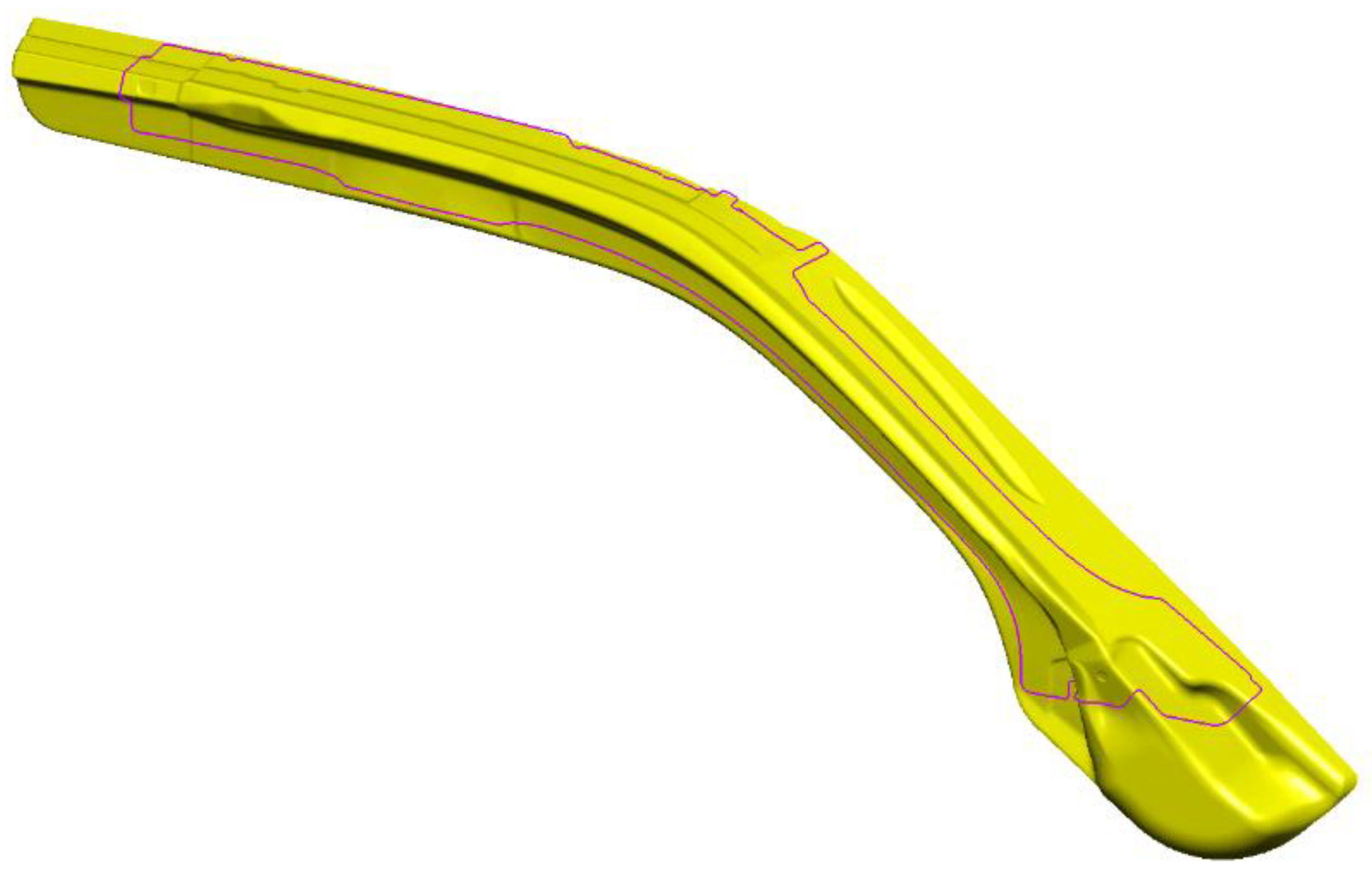
The simulation process consisted of three operations (stamping, trimming, and springback). Stamping was carried out as one continuous process in which the die moved at a speed of 100 mm/s. The blank was positioned between the die and the blankholder during holding. The die movement was set in the −z-direction at 300 mm until the blank was clamped. Subsequently, a blankholding force of 1900 kN was applied. The die and blankholder moved in the −z-direction until the tool was closed. After the part was fully formed, the trimming operation was performed. The trimming curve is shown in Figure 5.
4. Results
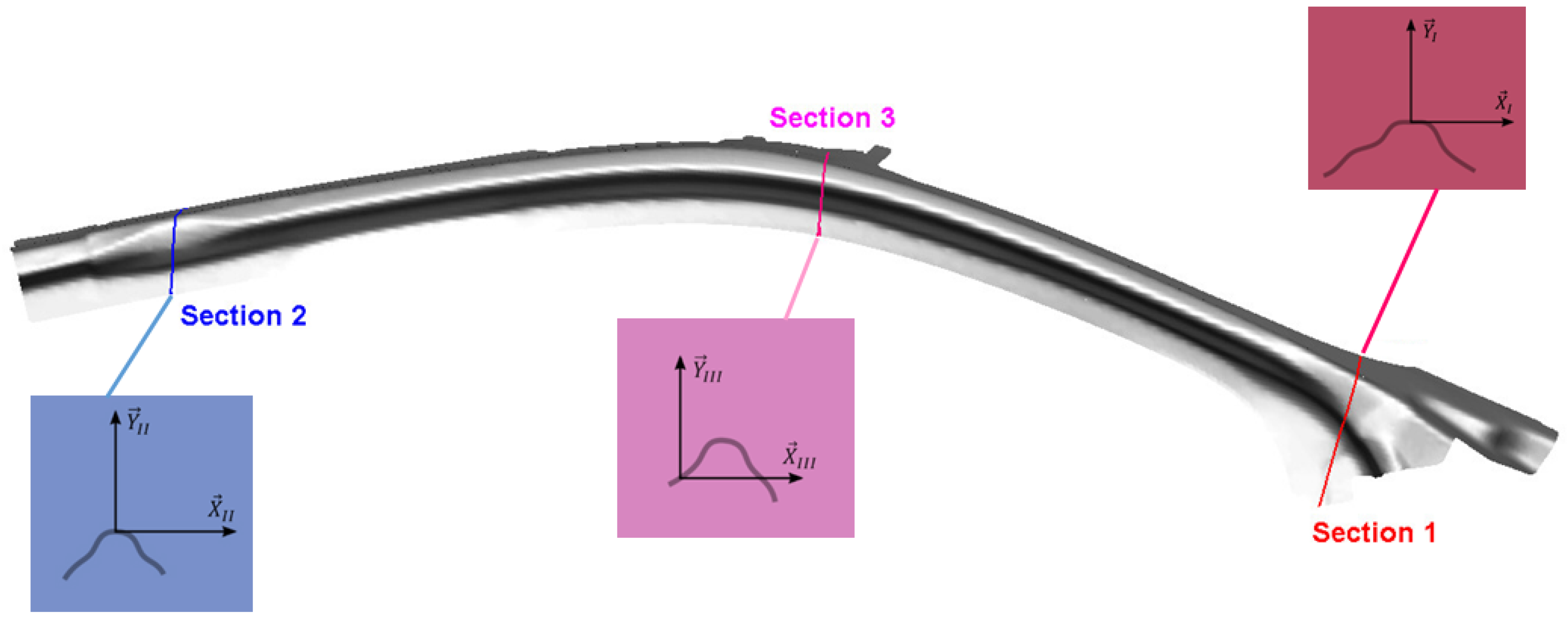
The results obtained from the numerical simulation were compared with the experimental ones. The springback was measured using locked nodes of the model. The stamped part profile and thickness were evaluated in three sections displayed in Figure 6. Section 1 is located on the right side of the part. This section passes through the hole, and due to the complex shape of the stamped part, the effect of the springback is quite significant in this area. The hole also runs through Section 2; this section is located on the left side of the part. The third section is located between section one and two. Figure 6 also shows the centres of the coordination systems used for profile evaluation. These centres were key for assembly purposes.
4.1. Profile Analysis
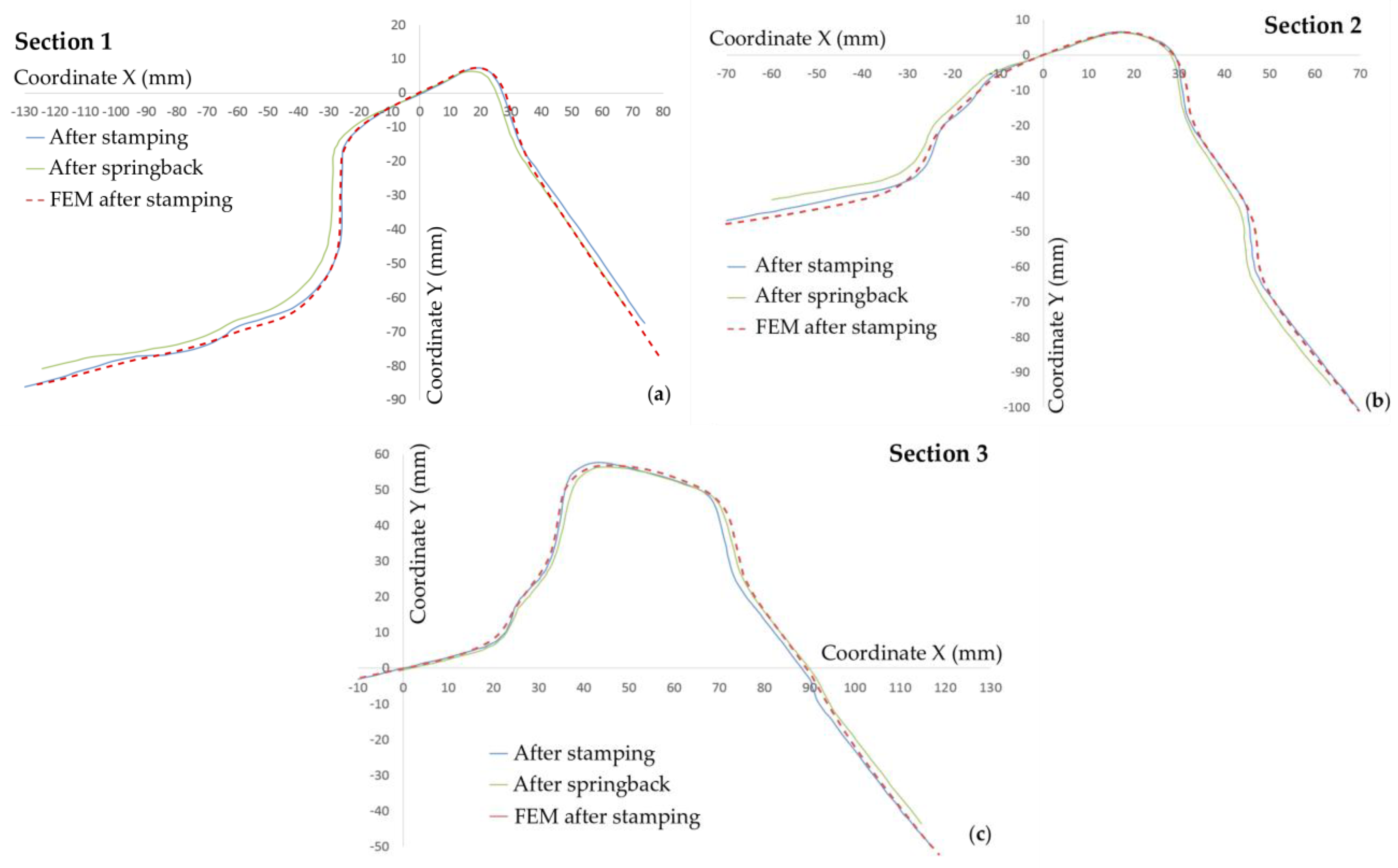
The profile of the part was measured before and after springback. Since the stamped part copies the shape of the die, the profiles after stamping were almost identical for every material model. Good correlation of the experimental and numerical results can be observed after stamping. The comparison of the experimental results and the FEM simulation after springback for each section is shown in Figure 7. Subsequently, the FEM results for each yield function after springback were also compared.
The deviations from the experimental results were measured on the left and on the right side of the sections. For assembly purposes, the deviation was measured in mm. Due to the difficulty of using conventional methods for springback measurement, the MATLAB system was implemented into the evaluation process. A simple program in the MATLAB environment was developed by the authors, which made it possible to measure the springback more accurately and easily. At first, a section was imported into the program, and the coordinate system was defined. Then, by selecting one point on the arm, a straight line parallel to the X-axis was created. Further points could only be created on this line, and the distance between each point was evaluated.
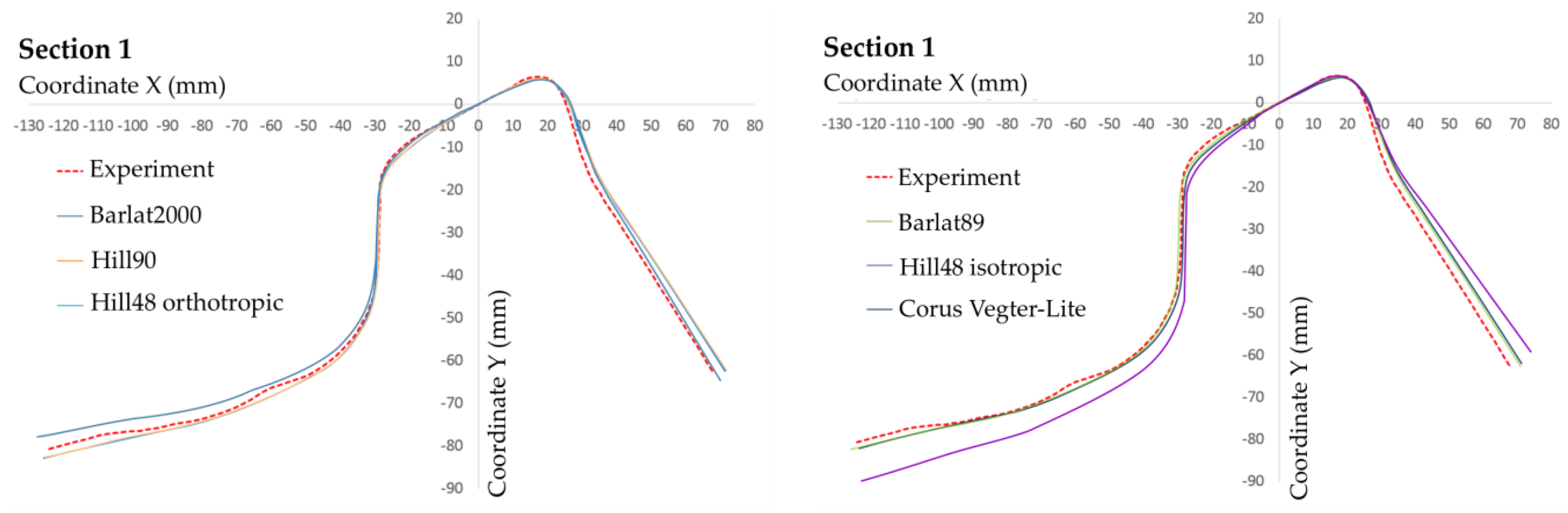
Figure 8 shows the experimental results and results from the numerical simulation in Section 1. Deviation from the experimental results for every yield function is shown in Table 7. A positive value means that the numerical simulation predicted a higher springback value than the experimental ones, and a negative value means that the simulation value was lower than the experimental ones. From these values, the average value of springback was calculated by the following equation:
where XL is the offset for the left side of the part and XR is the offset for the right side of the part.
The lowest average deviation of 1.21 mm was measured when the Barlat89 yield function was used. Yield functions Barlat2000 and Vegter-Lite had average deviations of 2.12 and 1.63, also showing very good correlation with the experimental results. The highest average deviation of 5.44 mm was measured for the isotropic Hill48 yield function. In this function, the anisotropy of the material was not considered.
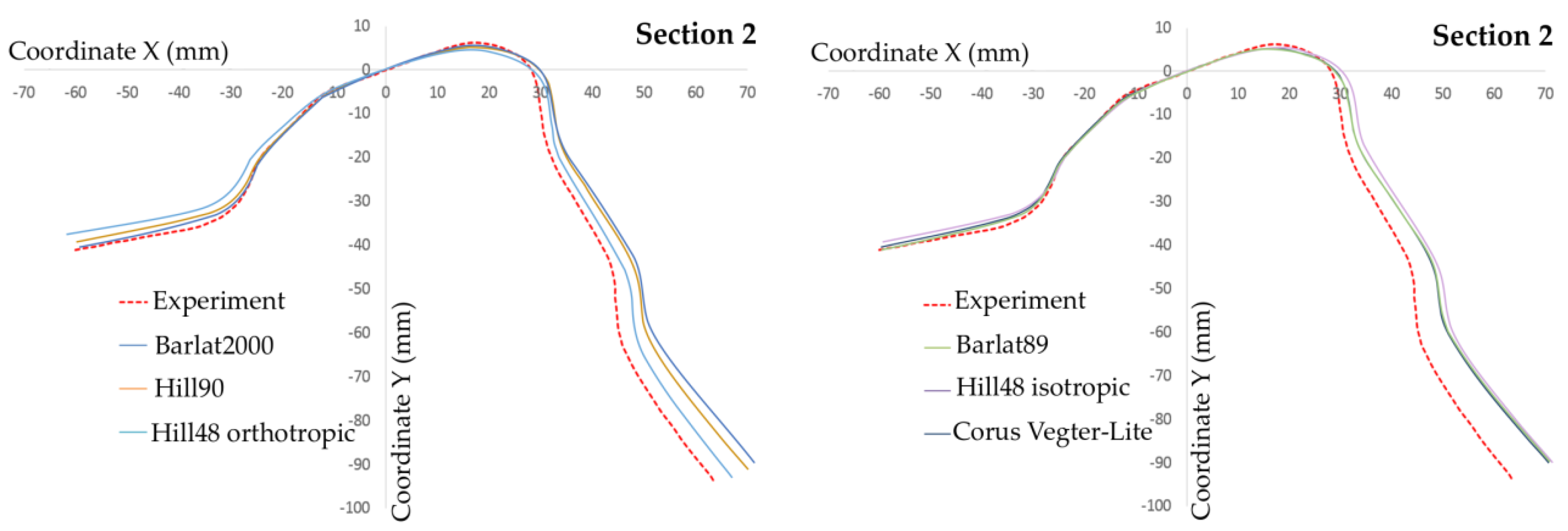
In Section 2 (Figure 9), greater deviation of the numerical springback values from the experimental ones can be seen on the right side of the profile. The reason is the shape of the part. Springback did not appear so significantly on the left side of the part where the material is compressed. The results are displayed in Table 8. In this section, the material model with the Vegter-Lite yield function showed the lowest average value of deviation: 2.65 mm. The Barlat89 yield function with 2.68 mm average deviation also shows good correlation. The other material models show very similar results, but the isotropic Hill48 method shows the highest deviation (3.51 mm) from the experimental results.
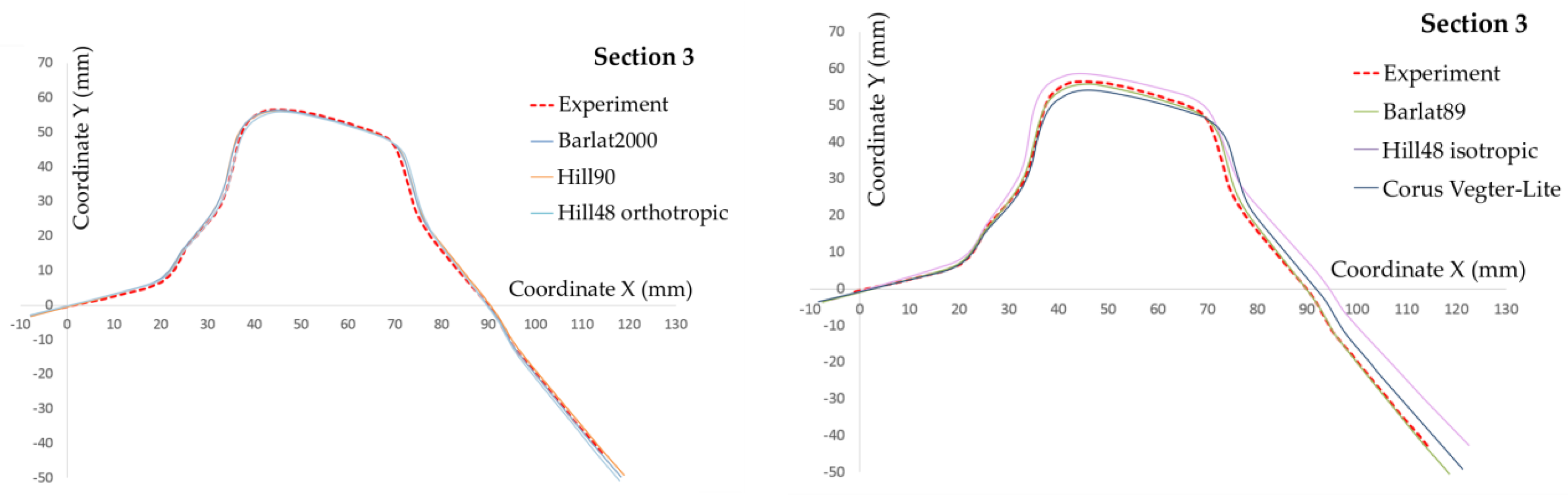
In the third section, the deviation was measured only on the right side because, on the left side, the deviation was too low, as shown in Figure 10. In this section, the best correlation was achieved with the Barlat yield functions, where the Barlat2000 deviation was 0.21 mm and the Barlat89 deviation was 0.32 mm. The highest deviation of 5.26 mm was measured for the isotropic Hill48 yield function. The results for all the material models are shown in Table 9.
4.2. Thickness Analysis
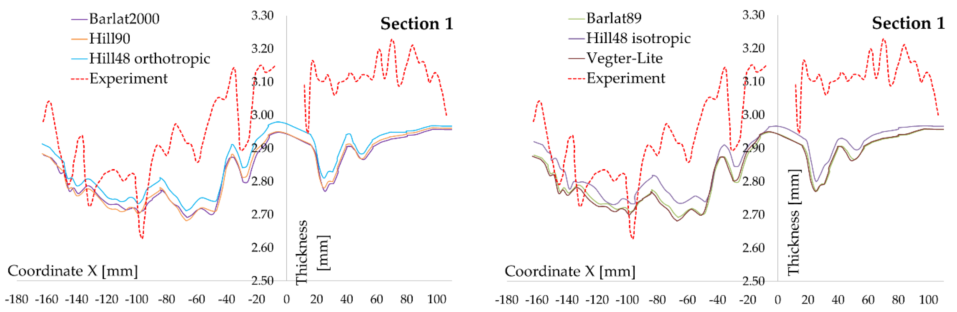
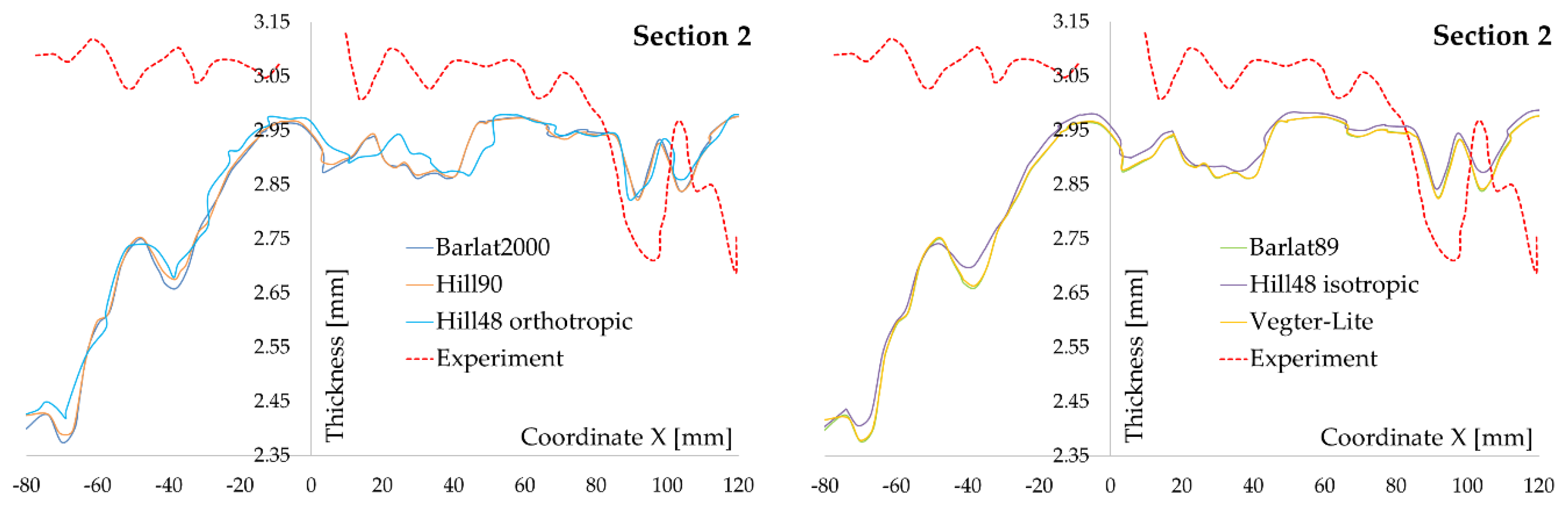
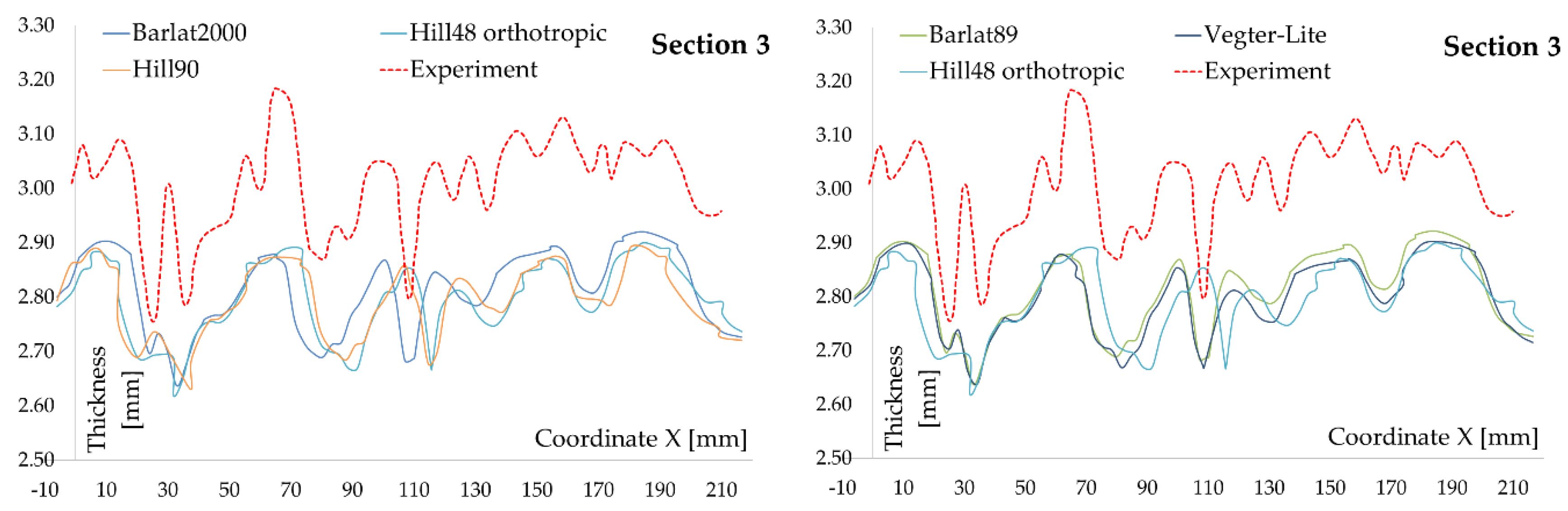
The next investigated parameter in this work was thickness, which was also measured in mentioned sections. The thickness of the material can significantly influence the accuracy of the FEM prediction. Since shell elements, which were used in this work, are suitable for thicknesses up to 1 mm, the volume element should give better results. However, in the FEM software, it is possible to define the volume elements for only the Hill48 and Barlat2000 yield functions. For comparison purposes of all previously mentioned yield functions, the models must have shell elements. Figure 11, Figure 12 and Figure 13 show comparisons of the experimental and FEM results in each section.
From the results of the thickness distribution in the individual sections, it is clear that the material models with the Barlat (Barlat89 and Barlat2000) yield functions, and the Vegter-Lite yield function shows very similar results. Although the description of the yield function and the amount of data needed for their definition is different between those models, the results of the thickness distribution were practically the same. The Hill48 model, either isotropic or orthotropic, exhibited significant deviations. The average values of thickness are shown in Table 10. The experimental results show a higher average thickness than the thickness data obtained by the FEM simulation.
4.3. Computation Time
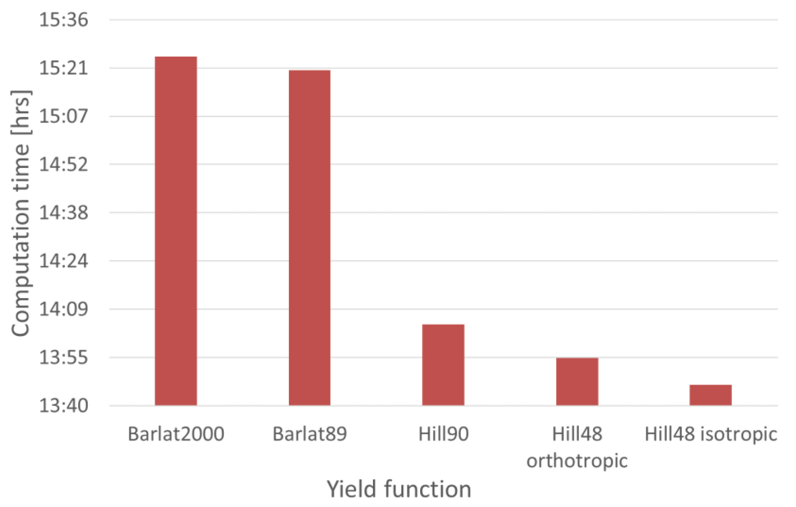
With the increased complexity of the yield function formulation and, thus, with the increased number of necessary variables, the calculation time was increased. For the Hill48 isotropic model, where the anisotropy of material was not considered, the computation took around 13 h and 47 min. For the Hill48 orthotropic and Hill90 models, where the anisotropy of the material was considered, the computation time took 14 h. In the Barlat yield functions, where the material’s crystallographic structure was considered, the computation time increased significantly to around 15 h and 20 min. The Vegter-Lite yield function achieved a similar accuracy and computation time as the Barlat material models. Figure 14 shows the comparison of the computation times for each yield function.
5. Conclusions
The accuracy of the springback prediction is one of the most challenging problems in the numerical simulation of forming processes. In the present article, the influence of the yield function on the accuracy of springback prediction with the use of numerical simulation was investigated. Three sections were defined on the formed part. In these sections, the thicknesses of the profile of the stamped part after springback calculation were evaluated. After the stamping operation, for all the examined yield functions, the sheet metal copied the shape of the die. Visible differences can be seen after cutting and springback calculation. The results of the Barlat2000, Barlat89, and Vegter-Lite yield functions were in good correlation with the experimental results. Hill’s yield functions (Hill90, isotropic Hill48, and anisotropic Hill48) were not as accurate as the yield functions mentioned above. Barlat’s yield functions takes into account the material’s crystallographic structures. The Barlat89 yield function, with an average deviation of 1.40 mm from experimental results of springback, is not suitable for materials with strong anisotropy [26]. Additionally, this model cannot capture the change of yield stress and the Lankford coefficient values. However, the advantage of this function lies in its simple mathematical description, and in the ability of the accurate plastic behaviour prediction (yield locus) of aluminium alloys, thus, the results of the Barlat89 model are more accurate than the results obtained with the use of Hill’s yield functions. The Barlat2000 yield function is an improved version of the Barlat89 model, but the description of this improved model in the numerical simulation is more difficult. This is the reason why this function is not used as much in industrial practice. The experimental thickness values were higher than the predicted ones in all cases. From the results of the thickness distribution in the individual sections, it is clear that the yield functions of the Barlat’s family and Vegter-Lite yield function show very similar results. Although the description of the yield function and the amount of data needed for their definition is different between those models, the results of the thickness distribution were practically the same. The Hill48 model, either isotropic or orthotropic, exhibited significant deviations. This can be attributed to the shell elements used in the numerical simulation or to the Voce isotropic hardening law. However, the Voce hardening law exhibited good correlation with the experimentally measured FLC (forming limit curve). One of the results of the work is that the combination of the isotropic hardening law with the isotropic yield function did not achieve accurate springback prediction results. The combination of more advanced yield functions (Barlat2000, Barlat89 and Vegter-Lite) with the isotropic Voce hardening law improved the accuracy of the springback prediction, but the computation time was increased by approximately an hour. Additionally, it was found out that the investigated phenomena which are required for the determination of the kinematic hardening model, such as the change of Young’s modulus E, transient behaviour, work-hardening stagnation, and permanent softening, were not observed in the aluminium alloy studied in this work. Our research confirmed that in aluminium alloys, there are no appreciable changes in the Young’s modulus value.
Author Contributions
M.Š. and J.S. performed the numerical simulations; E.S., J.S., M.Š., P.M., and T.S. performed the results analysis; E.S., J.S, M.Š., and P.M. wrote the article; E.S. and J.S. designed the experiments.
Funding
This research was funded by the Slovak Research and Development Agency under grant number APVV-14-0834 and the Grant Agency under grant number VEGA 1/0441/17.
Acknowledgments
The authors are grateful for the support of experimental works to the Slovak Research and Development Agency under project APVV-14-0834 “Increasing the quality of cut-outs and effectiveness of cutting electric sheets” and the grant agency for the support of the project VEGA 1/0441/17 “Application of high-strength materials for exterior car body parts”.
Conflicts of Interest
The authors declare no conflict of interest.
References
- Jeswiet, J.; Geiger, M.; Engel, U.; Kleiner, M.; Schikora, M.; Duflou, J. Metal forming progress since 2000. CIRP J. Manuf. Sci. Technol. 2008, 1, 2–17. [Google Scholar] [CrossRef]
- Banu, M.; Takamura, M.; Hama, T.; Naidim, O.; Teodosiu, C.; Makinouchi, A. Simulation of springback and wrinkling in stamping of a dual phase steel rail-shaped part. J. Mater. Process. Technol. 2006, 173, 178–184. [Google Scholar] [CrossRef]
- Chongthairungruang, B.; Uthaisangsuk, V. Springback prediction in sheet metal forming of high strength steels. Mater. Des. 2013, 50, 253–266. [Google Scholar] [CrossRef]
- Lei, D.; Xinyun, W.; Junsong, J.; Liangjun, X. Springback and hardness of aluminum alloy sheet part manufactured by warm forming processs using non-isothermal dies. Procedia Eng. 2017, 207, 2388–2393. [Google Scholar] [CrossRef]
- Mahabunphachai, S.; Koc, M. Investigations on forming of aluminum 5052 and 6061 sheet alloys at warm temperatures. Mater. Des. 2010, 31, 2422–2434. [Google Scholar] [CrossRef]
- Wagoner, R.H.; Lim, H.; Lee, M.G. Advanced Issues in springback. Int. J. Plast. 2013, 45, 3–20. [Google Scholar] [CrossRef]
- Yoshida, T.; Sato, K.; Hashimoto, K. Springback Problems in Forming of High-Strength Steel Sheets and Countermeasures; Nippon Steel Technical Report No. 103; Nippon Steel & Sumitomo Metal Corporation: Tokyo, Japan, May 2013. [Google Scholar]
- Toros, S.; Polat, A.; Ozturk, F. Formability and springback characterization of TRIP800 advanced high strength steel. Mater. Des. 2012, 41, 298–305. [Google Scholar] [CrossRef]
- Gau, J.T.; Kinzel, G.L. A New Model for Springback Prediction for Aluminum Sheet Forming. J. Eng. Mater. Technol. 2005, 127, 279–288. [Google Scholar] [CrossRef]
- Li, M.; Gan, W.; Wagoner, R.H. Sheet springback: Prediction and design. In Proceedings of the HSIMP 2007, High Speed Manufacturing Process, Senlis, France, 13–15 November 2007; pp. 1–7. [Google Scholar]
- Wagoner, R.H. Report: Advanced High Strength Workshop 2006; The Ohio State University: Columbus, OH, USA, 2006. [Google Scholar]
- Trzepiecinski, T.; Lemu, H.G. Effect of Computational Parameters on Springback Prediction by Numerical Simulation. Metals 2017, 7, 380. [Google Scholar] [CrossRef]
- Slota, J.; Siser, M.; Dvorak, M. Experimental and Numerical Analysis of Springback Behavior of Aluminum Alloys. Strength Mater. 2017, 49, 565–574. [Google Scholar] [CrossRef]
- Seo, K.Y.; Kim, J.H.; Lee, H.S.; Kim, J.H.; Kim, B.M. Effect of Constitutive Equations on Springback Prediction Accuracy in the TRIP1180 Cold Stamping. Metals 2017, 8, 18. [Google Scholar] [CrossRef]
- Mulidran, P.; Spisak, E.; Majernikova, J.; Sleziak, T.; Gres, M. Influence of forming method and process conditions on springback effect in the sheet metal forming simulation. Int. J. Eng. Sci. 2017, 6, 62–67. [Google Scholar] [CrossRef]
- Jung, J.B.; Jun, S.; Lee, H.S.; Kim, B.M.; Lee, M.G.; Kim, J.H. Anisotropic Hardening Behaviour and Springback of Advanced High-Strength Steels. Metals 2017, 7, 480. [Google Scholar] [CrossRef]
- Villuendas, A.; Jorba, J.; Roca, A. The Role of Precipitates in the Behavior of Young’s Modulus in Aluminum Alloys. Metall. Mater. Trans. A 2014, 45, 3857–3865. [Google Scholar] [CrossRef]
- Roca, A.; Villuendas, A.; Meíja, I.; Benito, J.B.; Llorca-Isern, N.; Lluma, J.; Jorba, J. Can Young’s modulus of metallic alloys change with plastic deformation? Mater. Sci. Forum 2014, 783–786, 2382–2387. [Google Scholar] [CrossRef]
- Allen, M.; Oliveira, M.; Hazra, S.; Adetoro, O.; Das, A.; Cardoso, R. Benchmark 2—Springback of a Jaguar Land Rover Aluminium. J. Phys. Conf. Ser. 2016, 734, 022002. [Google Scholar] [CrossRef]
- Dasappa, P.; Inal, K.; Mishra, R. The effects of anisotropic yield functions and their material parameters on prediction of forming limit diagrams. Int. J. Solids Struct. 2012, 49, 3528–3550. [Google Scholar] [CrossRef]
- Bruschi, S.; Altan, T.; Banabic, D.; Bariani, P.F.; Brosius, A.; Cao, J.; Ghiotti, A.; Khrasheh, M.; Merklein, M.; Tekkaya, A.E. Testing and modelling of material behaviour and formability in sheet metal forming. CIRP Ann.-Manuf. Technol. 2014, 63, 727–749. [Google Scholar] [CrossRef]
- Barlat, F.; Brem, J.C.; Yoon, J.W.; Chung, K.; Dick, R.E.; Lege, D.J.; Pourboghrat, F.; Choi, S.H.; Chu, E. Plane stress yield function for aluminum alloy sheets—Part 1: Theory. Int. J. Plast. 2003, 19, 1297–1319. [Google Scholar] [CrossRef]
- Slota, J.; Siser, M. Advanced Material Models for Stamping of AW 5754 Aluminum Alloy. Strength Mater. 2016, 48, 487–494. [Google Scholar] [CrossRef]
- Novy, J.; Vache, V.; Sobotka, J. Influence of used yield function in deep drawing simulation of highly anisotropic aluminum alloy. In Proceedings of the IDDGRG, Zurich, Switzerland, 2–5 June 2013; pp. 273–277. [Google Scholar]
- Vegter, H.; Horn, C.; Abspoel, M. The Corus-Vegter Lite Material model: Simplifying advanced material modeling. Int. J. Mater. Form 2009, 2, 511–514. [Google Scholar] [CrossRef]
- Slota, J.; Spisak, E. Comparison of the forming-limit diagram (FLD) models for drawing quality (DQ) steel sheets. Metabk 2005, 4, 249–253. [Google Scholar]
- Banabic, D. Advanced anisotropic yield criteria. In Sheet Metal Forming Processes, 1st ed.; Springer: Heidelberg/Berlin, Germany; Dordrecht, The Netherlands, 2010; pp. 76–87. ISBN 978-3-540-88112-4. [Google Scholar]
Figure 1.
The experimental stress-strain curves from the tensile test.

Figure 2.
The cyclic tension-compression experimental curve of AA6451-T4 [19].
Figure 2.
The cyclic tension-compression experimental curve of AA6451-T4 [19].

Figure 3.
The tool geometry in the PAM-Stamp 2G software.

Figure 4.
The rolling direction on the initial meshed blank.

Figure 5.
The trimming curve on the punch.

Figure 6.
The sections used for profile and thickness evaluation.

Figure 7.
The comparison of the part profile from FEM simulation after springback with the experimental results after stamping and springback in (a) Section 1; (b) Section 2; (c) Section 3.
Figure 7.
The comparison of the part profile from FEM simulation after springback with the experimental results after stamping and springback in (a) Section 1; (b) Section 2; (c) Section 3.

Figure 8.
The comparison of the yield functions in Section 1.

Figure 9.
The comparison of yield functions in Section 2.

Figure 10.
The comparison of yield functions in Section 3.

Figure 11.
The thickness distribution in Section 1.

Figure 12.
The thickness distribution in Section 2.

Figure 13.
The thickness distribution in Section 3.

Figure 14.
The computation time comparison.


Table 1.
The uniaxial tensile test data of the AA6451-T4 sheet [19].
Table 1.
The uniaxial tensile test data of the AA6451-T4 sheet [19].
| Orientation | Yield Strength σy (MPa) | Normal Anisotropy r (–) |
|---|---|---|
| 0° | 151.28 | 0.62 |
| 45° | 171.20 | 0.33 |
| 90° | 163.60 | 0.80 |
| Average value | 164.32 | 0.52 |
Table 2.
The elastic mechanical properties of AA66451-T4 [19].
Table 2.
The elastic mechanical properties of AA66451-T4 [19].
| Sample | Density, ρ (g·cm−3) | Young´s Modulus, E (GPa) | Poisson´s Ratio, v |
|---|---|---|---|
| AA6451-T4 | 2.7 | 70.0 | 0.3 |
Table 3.
The equal biaxial tension test data [19].
Table 3.
The equal biaxial tension test data [19].
| Biaxial Yield Stress σb (MPa) | Biaxial Anisotropy rb (-) |
|---|---|
| 153.60 | 0.55 |
Table 4.
The material constants for the Barlat89 yield function (m = 8.0).
| a | c | h | p |
|---|---|---|---|
| 1.3033 | 0.9556 | 0.9247 | 0.8465 |
Table 5.
The material constants for the Barlat2000 yield function (a = 8.0).
| a1 | a2 | a3 | a4 | a5 | a6 | a7 | a8 |
|---|---|---|---|---|---|---|---|
| 1.065173 | 0.841891 | 0.960059 | 0.958652 | 1.034037 | 1.027112 | 0.838988 | 0.877033 |
Table 6.
The parameters for the Voce hardening curve.
| A (MPa) | B (MPa) | C (–) |
|---|---|---|
| 359.093260 | 169.310139 | 9.374256 |
Table 7.
The results of springback in Section 1.
| Yield Function | Left Side Offset (mm) | Right Side Offset (mm) | Yield Function | Left Side Offset (mm) | Right Side Offset (mm) |
|---|---|---|---|---|---|
| Barlat2000 | +3.36 | +0.88 | Barlat89 | −1.28 | +1.15 |
| Hill90 | −2.14 | +3.77 | Hill48 isotropic | −9.29 | +3.53 |
| Hill48 orthotropic | −1.85 | +4.51 | Vegter-Lite | −1.67 | +1.59 |
Table 8.
The results of springback in Section 2.
| Yield Function | Left Side Offset (mm) | Right Side Offset (mm) | Yield Function | Left Side Offset (mm) | Right Side Offset (mm) |
|---|---|---|---|---|---|
| Barlat2000 | +0.45 | +5.79 | Barlat89 | −0.20 | +5.15 |
| Hill90 | +1.62 | +4.48 | Hill48 isotropic | +1.56 | +5.46 |
| Hill48 orthotropic | +3.78 | +2.21 | Vegter-Lite | +0.04 | +4.90 |
Table 9.
The results of springback in Section 3.
| Yield Function | Right Side Offset (mm) | Yield Function | Right Side Offset (mm) |
|---|---|---|---|
| Barlat2000 | −0.21 | Barlat89 | −0.32 |
| Hill90 | −0.75 | Hill48 isotropic | +5.26 |
| Hill48 orthotropic | +0.37 | Vegter-Lite | +1.97 |
Table 10.
The comparison of the average thickness of each section.
| Barlat2000 | Barlat89 | Vegter-Lite | Hill90 | Hill48 Orthotropic | Hill48 Isotropic | Experiment | |
|---|---|---|---|---|---|---|---|
| Section 1 | 2.825 | 2.828 | 2.826 | 2.828 | 2.834 | 2.858 | 2.980 |
| Section 2 | 2.856 | 2.847 | 2.853 | 2.852 | 2.847 | 2.859 | 2.991 |
| Section 3 | 2.809 | 2.810 | 2.792 | 2.798 | 2.797 | 2.809 | 2.990 |
© 2018 by the authors. Licensee MDPI, Basel, Switzerland. This article is an open access article distributed under the terms and conditions of the Creative Commons Attribution (CC BY) license (http://creativecommons.org/licenses/by/4.0/).
Share and Cite
MDPI and ACS Style
Mulidrán, P.; Šiser, M.; Slota, J.; Spišák, E.; Sleziak, T. Numerical Prediction of Forming Car Body Parts with Emphasis on Springback. Metals 2018, 8, 435. https://doi.org/10.3390/met8060435
AMA Style
Mulidrán P, Šiser M, Slota J, Spišák E, Sleziak T. Numerical Prediction of Forming Car Body Parts with Emphasis on Springback. Metals. 2018; 8(6):435. https://doi.org/10.3390/met8060435
Chicago/Turabian StyleMulidrán, Peter, Marek Šiser, Ján Slota, Emil Spišák, and Tomáš Sleziak. 2018. "Numerical Prediction of Forming Car Body Parts with Emphasis on Springback" Metals 8, no. 6: 435. https://doi.org/10.3390/met8060435
Note that from the first issue of 2016, this journal uses article numbers instead of page numbers. See further details here.