Simulation of Compound Rolls Produced by Electroslag Remelting Cladding Method

Abstract

Electroslag remelting cladding (ESRC) with a t-shape current carrying mold was adopted to make a compound roll including a working layer and mandrel. A comprehensive coupled transient model was established to reveal the basic phenomena of electromagnetic fields, flow fields, temperature fields, and multiphase flow. Meanwhile, the movement of the mandrel and working layer relative to the slag pool was simulated by dynamic mesh technology to reveal the interface bonding mechanism. The mechanism is as follows: The temperature of the mandrel increases and the mandrel melts slightly when the mandrel passes through the slag pool. The fusion layer is a mixture of molten steel of mandrel and working layer that is the connector between the mandrel and the working layer. Therefore, the interface bonding quality is dependent on a fusion layer that is affected by the voltage/power. The investigation indicates that the fusion layer thickness is between 2 and 4 mm in the condition of 40 V that benefits from obtaining a good interface bonding quality.

1. Introduction

Rolls play an important role in billet quality and production efficiency. At present, single material rolls are used in most of the rolling lines. However, single material rolls have three disadvantages. First, they are more expensive due to their higher alloy content. Second, the element segregation in a roll is serious due to a higher alloy content during the manufacture of the roll. Third, the service life of the roll is usually short because it is difficult to obtain both high surface hardness and core part toughness [1,2]. In light of this condition, centrifugal casting [3,4], a continuous pouring process for cladding (CPC) [5], and electroslag surfacing with the liquid metal method (ESSLM) [6] have been developed for the production of bimetallic compound rolls. Compared to single material rolls, the compound roll consists of internal material with toughness and external material with stronger hardness. Therefore, compound rolls have many advantages. The production cost is significantly reduced due to lower alloy content and no forging process. Further, not only is the heat treatment process simple, but also a higher inner toughness and outer hardness can be easily achieved. Finally, the compound roll has a long service life, which is obviously of economic benefit.

The centrifugal casting method is widely used in compound roll production due to its advantages including simplicity, efficiency and being free of pollutants [7]. Because the working layer contains a large number of heavy alloy elements such as molybdenum, vanadium, tungsten, and the like, element segregations will occur for strong centrifugal force. Therefore, cracks will easily form in the working layer because of uneven distribution of stress and hardness [8]. In 1992, CPC was reported by Hashimoto et al. [5]. High-speed steel series compound rolls produced by CPC are widely applied in the hot rolling lines [9]. By combining the advantages of conventional electroslag remelting (ESR) and CPC, ESSLM was developed by Medovar for manufacturing the compound roll [6]. But the process flow of ESSLM is complex. Based on ESR refining and melting, the electroslag remelting cladding (ESRC) method with ring electrode is proposed to produce compound rolls in this paper. The current carrying mold is advantageous to avoid much melting of the mandrel in this technology [10]. The high-temperature zone is close to the mold wall with the current carrying mold [11], which helps to control bonding interface quality. Therefore, the current carrying mold is more suitable for the production of compound rolls.

ESRC is one kind of the liquid-solid method. Regarding liquid–solid method, Takeuchi [12] and Sano [13] believe that fusion combination and metallic diffusion are the main way of the interface bonding mechanism. Rao [14] found that the combination quality was determined by the transition layer thickness which is influenced by the mandrel surface temperature. If the temperature of the mandrel surface is too low, not only will a good interface quality not form but also, slag inclusion will appear in the interface. On the other hand, a high surface temperature causes excessive melting of the mandrel that reduces the mechanical properties of the working layer.

The fusion layer thickness is used as the judge standards of the melting depth into the mandrel. A fusion layer of thickness 2~4 mm ensures good interface bonding quality and avoids excessive melting of the mandrel. A satisfactory fusion layer can only be achieved when the temperature of the mandrel surface is controlled within a suitable range. However, relevant information is still lacking, because ESRC is a novel technology and still does not have a large-scale industrialized application. Thus, a 2D axisymmetric transient mathematical model of ESRC is established to develop a better understanding of the basic phenomenon and study the effect of voltage/power on the interface bonding quality for future experiments. By using the dynamic mesh technology, the mandrel passing through the slag pool and the working layer moving downwards are simulated to obtain reasonable paraments for good interface bonding quality.

2. Process of ESRC

A schematic diagram of ESRC device mainly including slag, electrode ring, working layer, mandrel and t-shape current carrying mold is shown in Figure 1. The process flow of ESRC consists of following five steps. First, the mandrel was installed on the pulling device and arranged coaxially with the mold to obtain the uniform thickness of the working layer. Second, “wet start” in which the liquid slag melting in the lining electroslag furnace was poured into the gap between the mold and the mandrel was applied. Third, the consumable electrode ring was inserted into the slag pool, and a single circuit consisting of consumable electrode ring, slag, current carrying mold and power supply was switched on. When the current passed through the slag pool, the temperature of the slag pool increased rapidly due to the large quantity of joule heat. Fourth, the metal droplets generated by the electrode passed through the slag pool and formed a working layer under the cooling effect of the mandrel and mold. Meanwhile, the mandrel surface heated continuously by high-temperature liquid slag started to melt slightly. The mandrel and the working layer were connected to form a compound roll by the fusion layer that was made up of the mixture of molten 45 steel and Cr5 steel. Finally, the compound roll was pulled downward at a given speed. The current carrying mold and slag pool were stationary.

3. Mathematical Model

3.1. Geometric Model

Figure 2a is a two-dimensional axisymmetric model of the ESRC process. Mandrel (45 steel), air, electrode (Cr5), slag, solid slag skin and working layer were included. The current carrying mold was a t-shape. The upper part radius (R4) of the mold is 166 mm. The lower end radius (R5) is the radial distance between the symmetry axis and the roll edge which is 130 mm. The depth of liquid slag (D) is 70 mm. The mandrel radius (R1) is 75 mm, and the height is 480 mm. The electrode ring (B) thickness is 20 mm whose inner radius (R2), and outer radius (R3) are 85 mm and 105 mm, respectively. After pouring slag, a 1 mm thickness solid slag skin (F) is formed on the mandrel surface [15] shown in Figure 2a because of the mandrel’s cooling effect.

The dynamic mesh technique was employed to simulate the downward movement relative to the slag pool (D) of the compound roll including the mandrel (A) and the working layer (E). The mandrel-air (13), mandrel-slag (14) and mandrel-ingot (15) boundaries are set as the sliding interface to avoid grid errors in the withdrawal process. In Figure 2c the mandrel, air, slag pool and ingot are stationary at initial state. The interior zone is produced where the interface zone 1 and interface zone 2 overlap. When the mandrel slides downward relative to the air and slag pool, the interface zone 1 that comprise the boundary (13~15) extends beyond the interface zone 2. Meanwhile, additional wall zone for the portions of the boundary is created in Figure 2d by default [16]. The flux of the overlapping intersection between two interface zones can be computed through an interior zone. The boundary can also be set as coupled where interior zone exists. The flux and convection can be used for wall zone.

Dynamic layering technology is used to simulate the growth of the working layer. Therefore, the boundary of ingot bottom (7) was set as layering interface to add layers of cells adjacent to the ingot bottom (7) shown in Figure 2b. Obviously, the boundary of mandrel-ingot (15’) and ingot-lateral (6) lengthen in Figure 2d. The other boundaries were stationary. The thermal and electrical boundary conditions are summarized shown in

Table 1. Thermal and electrical boundary condition.

Air-slag: ${\epsilon }_{\mathrm{r}}=0.8$, $H=50\mathrm{W}\cdot {\mathrm{m}}^{-2}\cdot {\mathrm{K}}^{-1}$, $\frac{\partial \varphi }{\partial Z}=0$, $\frac{\partial A_{\mathrm{Z}}}{\partial Z}=A_{\mathrm{r}}=0$

Electrode-slag lateral: 1758 K, $\varphi =40\mathrm{V}$, $\frac{\partial A_{\mathrm{r}}}{\partial r}=A_{\mathrm{z}}=0$

Electrode-slag: 1758 K, $\varphi =40\mathrm{V}$, $\frac{\partial A_{\mathrm{Z}}}{\partial z}=A_{\mathrm{r}}=0$

Ingot-slag: interior

Mold bottom: 1650 K, $\frac{\partial \varphi }{\partial Z}=0$, $\frac{\partial A_{\mathrm{Z}}}{\partial Z}=A_{\mathrm{r}}=0$

Ingot lateral: $H=500\mathrm{W}\cdot {\mathrm{m}}^{-2}\cdot {\mathrm{K}}^{-1}$, $\frac{\partial \varphi }{\partial r}=0$, $\frac{\partial A_{\mathrm{r}}}{\partial r}=A_{\mathrm{z}}=0$

Ingot bottom: $H=300\mathrm{W}\cdot {\mathrm{m}}^{-2}\cdot {\mathrm{K}}^{-1}$, $\frac{\partial \varphi }{\partial Z}=0$, $\frac{\partial A_{\mathrm{Z}}}{\partial z}=A_{\mathrm{r}}=0$

Slag-lateral: 1650 K, $\varphi =0\mathrm{V}$, $\frac{\partial A_{\mathrm{r}}}{\partial r}=A_{\mathrm{z}}=0$

Mandrel-slag, mandrel-ingot: coupled, $\frac{\partial \varphi }{\partial r}=0$, $\frac{\partial A_{\mathrm{r}}}{\partial r}=A_{\mathrm{z}}=0$

.

3.2. Hypothesis of Model

ESRC is a complicated process including electromagnetic fields, flow fields and temperature fields. Moreover, the working layer solidifying on the mandrel surface moves downwards with the mandrel. To simplify the calculation, the following assumptions are made:

(1)

As far as the physical parameters of slag and Cr5 steel are concerned, only thermal conductivity is related to temperature, and the rest is constant.

(2)

The melting depth into the mandrel surface was considered as the thickness of the fusion layer.

(3)

To improve the convergence rate, the electrical conductivity of Cr5 steel is set as zero.

(4)

The electrode melting rate can reach a constant within 2 min. During this period, the melting rate can be neglected, so the withdrawal starts from the steady state of the melting rate.

(5)

The volume of molten steel that melts from the mandrel surface is so small that its effect on the process can be ignored.

3.3. Equation

3.3.1. Electromagnetic Field Equation

Kharicha et al. [17] and Karimi-Sibaki et al. [18] believed that the $A-\phi$ magnetic vector potential method is more accurate for solving electromagnetic field in ESR simulation. Therefore, the magnetic vector potential method is used to solve the electromagnetic field.

The current density ($J$) equation includes two parts:

$$J=-\sigma \nabla \phi -\sigma \frac{\partial A}{\partial \tau }$$

(1)

The current is decided by the electric conductivity of the material ($\sigma$) and electric scalar potential ($\phi$). The direct current (DC) is applied. Therefore, the second term in the right-hand side of Equation (1) is neglected because there is no effect of eddy current. Thus, Equation (1) can be written as:

$$J=-\sigma \nabla \phi$$

(2)

To calculate the electric potential, Equation (2) is combined with the electric current conservation Equation (3).

$$\nabla \cdot J=0$$

(3)

Magnetic field strength ($B$):

$$\nabla \times A=B$$

(4)

Ampere-Maxwell’s Theorem:

$$\nabla \times \left(\frac{1}{\mathsf{\mu }}B\right)=J$$

(5)

The magnetic permeability $\mathsf{\mu }$ is assumed to be a constant $1.257\times {10}^{-6}$.

The magnetic vector potential equations can be deduced from Equations (4) and (5):

$$\frac{1}{\mathsf{\mu }}\nabla \left(\nabla \cdot A\right)-\frac{1}{\mathsf{\mu }}{\nabla }^{2}A=J$$

(6)

Note that, to obtain a unique solution for Equation (6), the coulomb gauge (7) is used [19].

$$\nabla \cdot A=0$$

(7)

The basic equation for the vector magnetic field is thus obtained:

$${\nabla }^{2}A=-\mathsf{\mu }J$$

(8)

Joule heating ($Q$):

$$Q={\left|J\right|}^2\cdot {\sigma }^{-1}$$

(9)

Lorentz force ($F_{\mathrm{loc}}$):

$$F_{\mathrm{loc}}=J\times B$$

(10)

The boundary conditions of the electromagnetic field are more complex. The electric potential of the electrode and the conductive mold wall are 40 V and 0 V, respectively. The remaining boundary is set as insulation. The continuity of magnetic vector potential A_Z is applied at the following interfaces: air-slag, slag-ingot, slag-bottom, and electrode-slag and the value of A_r is zero at these boundaries. Furthermore, the other boundaries take the value zero for the axial component of the magnetic vector potential. Meanwhile, a magnetic vector potential flux of zero is used at these boundaries.

3.3.2. Multiphase Flow Equation

Multiphase flow is calculated with the Volume of Fluid (VOF) method [20] that is defined as the ratio ${\alpha }_{\mathrm{q}}$ of the target fluid volume to the mesh volume. If the value of this function on each grid is figured out, the movement interface can be tracked. ${\alpha }_{\mathrm{q}}$ is calculated from the continuity equation:

$$\frac{\partial }{\partial \tau }\left({\alpha }_{\mathrm{q}}{\rho }_{\mathrm{q}}\right)+\nabla \cdot \left({\alpha }_{\mathrm{q}}{\rho }_{\mathrm{q}}{\upsilon }_{\mathrm{q}}\right)=0$$

(11)

$${\displaystyle \sum _{\mathrm{q}}^n{\alpha }_{\mathrm{q}}}=1$$

(12)

$${\displaystyle \sum _{\mathrm{q}}^n{\alpha }_{\mathrm{q}}}{\rho }_{\mathrm{q}}=\rho$$

(13)

The density ($\rho$) of each cell is the sum of each phase density (${\rho }_{\mathrm{q}}$). Other material properties are treated similar to the density.

3.3.3. Fluid Flow Equation

The flow is modeled with the continuity equation and time-averaged Navier–Stokes equation:

$$\frac{\partial \rho }{\partial \tau }+\nabla \cdot v=0$$

(14)

$$\frac{\partial \rho v}{\partial \tau }+\rho \left(v\cdot \nabla \right)v=-\nabla P+\nabla \cdot \left({\mu }_{\mathrm{eff}}\cdot \nabla v\right)+\rho g+S$$

(15)

$$S=F_{\mathrm{loc}}+F+{\rho }_{0}g\beta (T-T_0)$$

(16)

where $P$ is the pressure, ${\mu }_{\mathrm{eff}}$ is the dynamic viscosity, $v$ is the velocity, $g$ is the gravity, and $S$ is the source term including Lorenz force ($F_{\mathrm{loc}}$), interfacial tension $F$ and thermal buoyancy. The interfacial tension $F$ has a significant impact on droplet formation and slag/metal surface fluctuation [21]. The last item on the right of Equation (16) is the Boussinesq approximation because of the buoyancy in the slag pool. $\beta$ is the thermal expansion coefficient, ${\rho }_0$ and $T_0$ are reference density and reference temperature, respectively. Jardy et al. [22] found that the movement of the slag and metal in the ESR process is not strongly turbulent. Therefore, the Re-Normalization Group (RNG) $\kappa -\epsilon$ turbulent model is appropriate and accurate.

The Air-slag interface is considered as a free–slip condition. Additionally, the non-slip boundary condition is applied to other boundaries of the slag pool.

3.3.4. Temperature Field Equation

Convection heat transfer equation of the slag pool:

$$\rho C_{\mathrm{p}}\frac{\partial T}{\partial \tau }+\rho C_{\mathrm{p}}\left(v\cdot \nabla T\right)=\nabla \cdot K_{\mathrm{eff}}\nabla T+Q$$

(17)

where $C_{\mathrm{p}}$ is the slag thermal capacity, T is the temperature and $K_{\mathrm{eff}}$ is the effective conductivity.

The temperature field of the mandrel is obtained by solving an enthalpy ($H$) conservation equation.

$$H=C_{\mathrm{e}}T+f_{1}L$$

(18)

$$\frac{\partial \rho H}{\partial \tau }+\nabla \cdot \left(\rho v_{\mathrm{e}}H\right)=K_{\mathrm{e}}\nabla T$$

(19)

$$f_1=\frac{T-T_{\mathrm{s}}}{T_{\mathrm{l}}-T_{\mathrm{s}}}$$

(20)

where $C_{\mathrm{e}}$ is the specific heat capacity of the mandrel, $v_{\mathrm{e}}$ is the mandrel moving speed.

After pouring slag, the initial temperature of the slag is set as 1823 K. Because of the mandrel’s cooling effect, a 1 mm thickness solid slag skin (F) is formed on the mandrel surface [15] shown in Figure 2a. The temperature of the mandrel and surrounding air is 300 K. The temperature of electrode–slag (3) and electrode–slag–lateral (2) in Figure 2b is the liquidus temperature of the Cr5 steel. The temperature of slag lateral (8) and mold bottom (5) are the liquidus temperature of the slag. The temperature of 300 K is applied for air-up (10) and air lateral (9). The interface between the slag pool and the mandrel is considered to be coupled. The radiation and convection are taken into account for the boundary electrode–air/air–slag/mandrel–air.

3.3.5. Dynamic Mesh

Dynamic mesh is used to simulate the downward movement of the mandrel and working layer. To ensure the accuracy, the moving speed ($v_{\mathrm{g}}$) of the mesh must be applied to all the conservation equations [17].

$$\frac{d}{dt}{\displaystyle \underset{V}{\int }\rho \varphi dV}+{\displaystyle \underset{\partial V}{\int }\rho \varphi }(v-v_{\mathrm{g}})\cdot d{A}_1={\displaystyle \underset{\partial V}{\int }\Gamma \nabla \varphi \cdot }d{A}_1+{\displaystyle \underset{V}{\int }{S}_{\varphi }}dV$$

(21)

where $\varphi$ is a general scalar, $V$ is a control volume, $v$ is the flow velocity vector, $v_{\mathrm{g}}$ is the moving mesh velocity, $\Gamma$ is the diffusion coefficient, and $S_{\varphi }$ is the source term of $\varphi$. Here, $\partial V$ is used to represent the boundary of the control volume, $V$.

$$\frac{dV}{dt}={\displaystyle \underset{\partial V}{\int }{v}_{\mathrm{g}}}\cdot d{A}_1={\displaystyle \sum _{\mathrm{j}}^{n_f}{v}_{\mathrm{g},\mathrm{j}}}\cdot A_1{}_{\mathrm{j}}$$

(22)

where $n_f$ is the number of faces on the control volume and $A_1{}_{\mathrm{j}}$ is the $\mathrm{j}$ face area vector.

3.4. Physical Parameter

The detailed physical parameters are listed in

Table 2. Physical parameters of slag/steel/air.

Item	Parameter	Value
Slag	Density	2850 kg/m3
	Viscosity	0.01 kg/m/s
	Specific heat, liquid Cp	1404 J/kg/K
	$\beta$	9 × 10−5/K
	Emissivity of slag	0.6
Cr5	Density	7800 kg/m3
	Viscosity of molten steel	0.006 kg/m/s
	Specific heat, liquid Cp	760 J/kg/K
	Thermal conductivity of solid steel	26.5 W/m/K
	Thermal conductivity of molten steel	32.5 W/m/K
	Steel liquidus temperature	1758 K
	Steel solidus temperature	1683 K
	Latent heat of solidification	247,000 J/kg
45#	Density	7850 kg/m3
	Viscosity of molten steel	0.006 kg/m/s
	Specific heat, liquid Cp	700 J/kg/K
	Thermal conductivity of solid steel	25.1 w/m/K
	Thermal conductivity of molten steel	33.2 w/m/K
	Steel liquidus temperature	1760 K
	Steel solidus temperature	1700 K
	Latent heat of solidification	228,000 J/kg
Air	Density	1.2 kg/m3
	Viscosity	1.7 × 10−5 kg/m/s
	Specific heat, liquid Cp	1000 J/kg/K
	Thermal conductivity	0.02 W/m/K

. The thermal conductivity of the slag below 1473 K is shown in the Formula (23) by Dong et al. [23] experimental data:

$$\lambda =\{\begin{array}{ll}1.180\times {10}^{-3}（T-273)+1.004& 673\mathrm{K}\le \mathrm{T}\le 1473\mathrm{K}\\ 6& \mathrm{T}>3\mathrm{K}\end{array}$$

(23)

3.5. Process Parameters

The process parameters from the semi-industrial experiment are in

Table 3. Electrode drop velocity with different process parameters.

Case	Voltage (V)	Electrode Insertion Depth (mm)	Electrode Descending Velocity (mm/s)	Withdrawal Velocity (mm/s)
1	42	20	0.312	0.105
2	40	20	0.257	0.087
3	38	20	0.223	0.075

.

4. Solution Method

In Figure 3, the Magnetohydrodynamics (MHD) module is used to solve the electric field, and then the User Defined Scalars (UDS) equation is used to solve the magnetic field. According to our experiments, the melting speed of the electrode tends to be a constant within two minutes. First, the electromagnetic field, the flow field and the temperature field are solved by iteration for 120 s. The total amount of steel melting in two minutes is ignored, so the dynamic mesh is turned on to drive the compound roll to slide down relative to the slag pool after two minutes. The melting rate calculated from the experiment is used for the velocity-inlet at the electrode-slag boundary to keep mass conservation.

5. Results and Discussion

5.1. Basic Phenomena

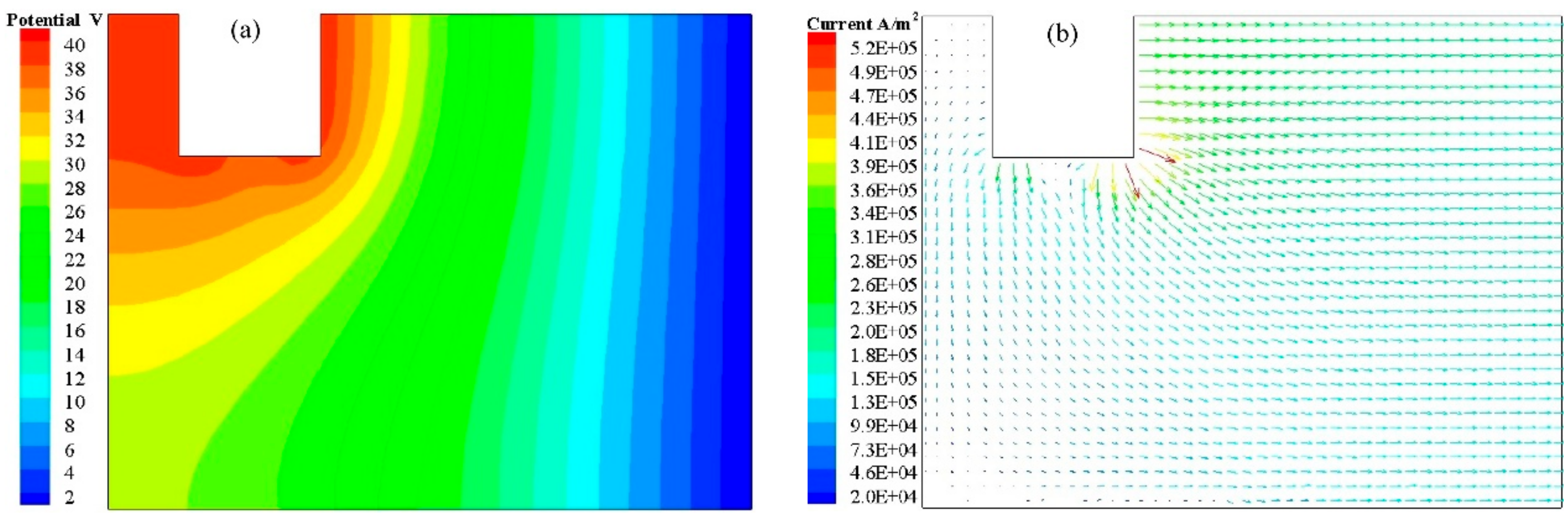
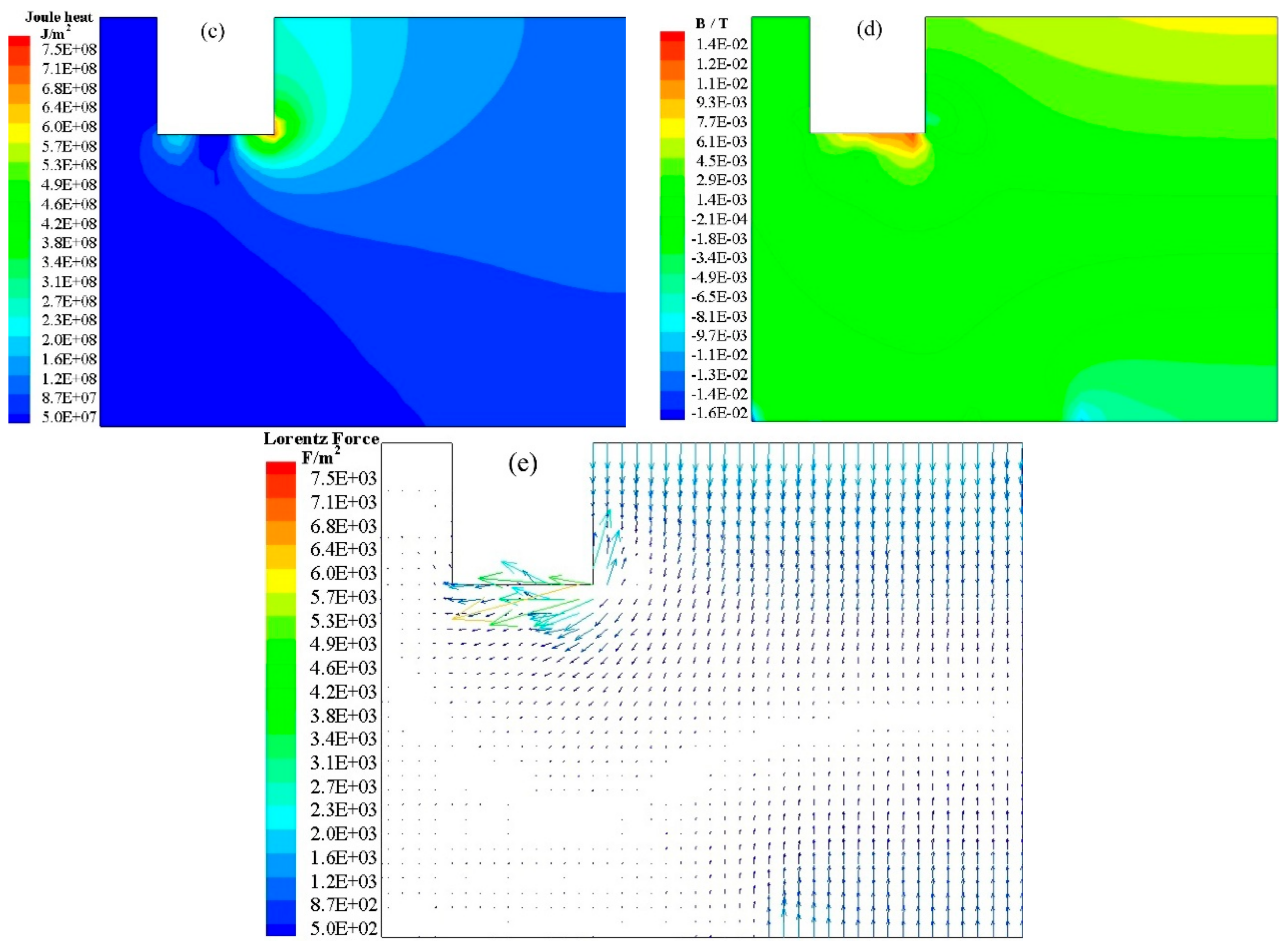
5.1.1. Electromagnetic Phenomena

A 2D axisymmetric model is established to develop a better understanding of the basic ESRC phenomenon. When the immersion depth of electrode into the slag pool is 20 mm in the condition of 40 V, the constant descending rate of electrode is 0.257 mm/s. In Figure 4, the electrical parameters are only analyzed in the slag pool because the conductive circuit is composed of the power supply, consumable electrode, slag pool and current carrying mold. The potential gradient is larger between the electrode and mold shown in Figure 4b. The maximum current density appearing on the electrode right corner is 52,500 A/m². The current density gradually decreases as the resistance increases. Thus, there is almost no current on the left side of the electrode. Joule heat density has a positive correlation with the current density, so the larger value of the joule heat density is near the right side of the electrode shown in Figure 4c. In Figure 4d, the magnetic flux density is complicated. The maximum B that lies on the lower right corner of the electrode is about 0.013 T. When the current passing through the slag pool comes across the magnetic field, the liquid slag will be subjected to Lorentz force. The cross-product of the maximum current and magnetic flux density leads to the maximum Lorentz force on the lower right corner of the electrode. The Lorentz force on both sides of the electrode is not symmetrical. In the right region of the slag pool, the Lorentz force directions of the upper part and lower part are opposite in Figure 4e.

5.1.2. Flow Field and Temperature Field

The flow field is mainly affected by Lorentz force, gravity and thermal buoyancy. As the slag is subjected to Lorentz force and the thermal buoyancy produced by joule heat, the slag pool moves clockwise on the right side of the electrode in Figure 5a. The temperature is highest in this zone because of higher joule heat density and vortex center. The temperature is lowest on the left side of the electrode due to lower joule heat density and weak heat transfer. Powerful Lorentz force mainly makes the slag flow counter-clockwise under the electrode which is helpful to obtain a uniform temperature field. The slag continuously exchanges heat with the mandrel which causes a decrease in slag temperature under the electrode. The reason for the weak flow in the lower right corner of the slag pool is the lack of thermal buoyancy and Lorentz force. The droplets do not move vertically downward under the electrode like that in traditional ESR [24] because of an unsymmetrical Lorentz force and flow field. Under the influence of gravity and the strong flow field of the slag, the droplets are driven to move counter-clockwise. Finally, the maximum velocity of the slag and droplets increases to 0.16 m/s in the lower left corner. Further, the molten steel with large momentum brings about larger interface fluctuation as in Figure 5c.

5.2. Interface Bonding Quality along the Height of the Compound Roll

As the electrode continuously melts, molten steel solidifying on the mandrel surface forms the working layer. The working layer and mandrel synchronously move down along the red arrow in Figure 6a, so the height of compound roll is increasing as shown in Figure 6a–e. The mandrel is divided into an infinite number of cross sections such as cross-section (M). During the withdrawal process, every cross section successively passes the 0~70 mm heating distance in the slag pool as shown in Figure 6a. The monitoring points are set up to record the temperature when the cross sections pass through the slag pool. They are stationary relative to the coordinate axis. The axial positions of 16 red temperature monitoring points are the heating distance that are 0, 10, 20, 30, 40, 50, 60 and 70 mm, respectively. The radial positions are at a 2 mm and 4 mm depth into the mandrel surface in turn. Lines (0~7) only represent the axial positions, not the radial positions. The starting height on the different monitoring points is 140~70 mm, and the end height is 460~390 mm, respectively. Therefore, the starting points and end points of eight temperature curves are different in Figure 7. But the length of the path lines (0~7) that are monitored on 16 different points is the same. Note that (A) point (2 mm, 270 mm) and (B) point (4 mm, 270 mm) are on the cross section (M).

The interface bonding quality is decided by the interface temperature. To reveal the change of interface bonding quality along the height of the compound roll, the interface temperature is recorded to analyze the interface bonding quality in the withdrawal process. Case 2 in Table 2 is introduced as an example. The temperature of cross sections at different mandrel heights is recorded in Figure 7 when cross sections pass through 16 monitoring points. In Figure 7a, the meaning of curve 70 mm is that the temperature of cross sections is recorded when the cross sections pass through the monitoring point of heating distance 70 mm. A large amount of heat is absorbed by the mandrel whose temperature rises rapidly due to the large temperature difference between the mandrel and slag in the early period. After the mandrel moves down by 20 mm, the reason why the surface temperature increases slowly is that the temperature difference decreases. When the mandrel drops by 60 mm, the solid slag gradually moves down with the mandrel which increases the thermal conductivity between the mandrel and liquid slag. Then, the temperature of each point begins to rise rapidly. After the mandrel is lowered by 90 mm, the temperature field is in a steady state, and the temperature of the mandrel at each monitoring points is the highest. The interface bonding quality depends on the fusion layer thickness that is controlled by the interface temperature. If the interface temperature is higher than the liquidus temperature and continues for enough time in withdrawal process, the fusion layer will form, and the interface quality will be better. In the early period, the interface quality is poor because the temperature of mandrel surface is lower than the liquidus temperature. In the steady state, the interface quality is controlled by the largest temperature that is dependent on Voltage/Power. Therefore, the effect of voltage/power on the interface bonding quality should be studied.

5.3. Impact of Voltage/Power on the Interface Bonding Quality

The interface bonding quality of the compound roll is dependent on the surface temperature. Therefore, the voltage/power, the most important factor on surface temperature, is studied. The maximum current density and joule heat density are linearly proportional to the voltage in Figure 8. As the voltage increases from 38 to 42 V in Figure 9, the maximum temperature of the slag pool increases from 1976 to 2025 K and the average temperature of the slag pool increases from 1858 to 1899 K, respectively. The temperature of the mandrel increases significantly with the increment of the slag pool temperature. In Figure 10, the maximum temperature of the mandrel surface increases from 1740 to 1800 K (above the liquidus temperature) that makes the mandrel surface move from no melting to completely melting. However, if the largest temperature of the mandrel surface is much higher than the liquidus temperature, mandrel excessively melts and mixes with the working layer, which will reduce the mechanical properties of the working layer. Therefore, the fusion layer thickness is set as the judge standards of the melting depth into mandrel surface. A reasonable fusion layer of thickness 2~4 mm will be obtained between 38 and 42 V.

To get a reasonable voltage, the temperature of (A) point and (B) point on cross-section (M) is recorded when they pass through the slag pool. In Figure 11a, as for 38 V, the 2mm depth into mandrel surface will not melt because its maximum temperature 1724 K is far below the liquidus temperature 1760 K. Under the condition of 40 V, a good metallurgical combination will form because the fusion layer thickness is within the range 2~4 mm. When two points pass by 40 mm, the temperature of 2 mm depth becomes close to the liquidus temperature, and the surface begins to melt slightly. The temperature is slightly higher than the liquidus temperature when the points are heated at the distance of 40~70 mm that makes the fusion layer of thickness 2 mm form. In Figure 11b, for the remaining 30 mm, the maximum temperature of 4 mm depth is 1736 K, which is lower than the liquidus temperature so the 4 mm thickness into mandrel will not melt. The synthetic properties of the compound roll are improved because the interfaces between the mandrel and working layer are connected by the fusion layer whose thickness is in the range of 2~4 mm. It is difficult to prevent the mandrel surface from melting sharply because the maximum temperature of 4 mm depth reaches 1769 K in the case of 42 V. In summation, 40 V is more suitable for actual industrial production.

6. Conclusions

An ESRC method with the current carrying mold is used to produce compound rolls. A 2D axisymmetric transient mathematical model is established, and MHD module together with UDS equation is used to solve the electromagnetic field. Related physical parameters and boundary condition functions are written by User Defined Functions (UDF). More importantly, to reveal the basic phenomena and the interface bonding mechanism, the movement of the mandrel and working layer is simulated by the dynamic mesh. The effect of voltage/power on interface bonding quality is also studied. The following conclusions are drawn:

(1)

The current density is mainly distributed between the electrode and the mold. The joule heat density is positively correlated with the current density, so the area between electrode and mold is the highest temperature zone. Under the electrode, the Lorentz force leads to a counter-clockwise flow which helps to uniform the temperature of slag pool as well as increase the temperature of the mandrel.

(2)

The mandrel is divided into infinite cross sections. In the transient withdrawal process, the temperature of cross sections is analyzed to study the change of interface bonding quality along compound roll height. The temperature of mandrel surface increases until the temperature field reaches steady. The mandrel and working layer are separated in the early period because the temperature of mandrel surface is below the liquidus temperature. In steady state, the interfacial quality is dependent on the interface temperature that is affected by the voltage/power.

(3)

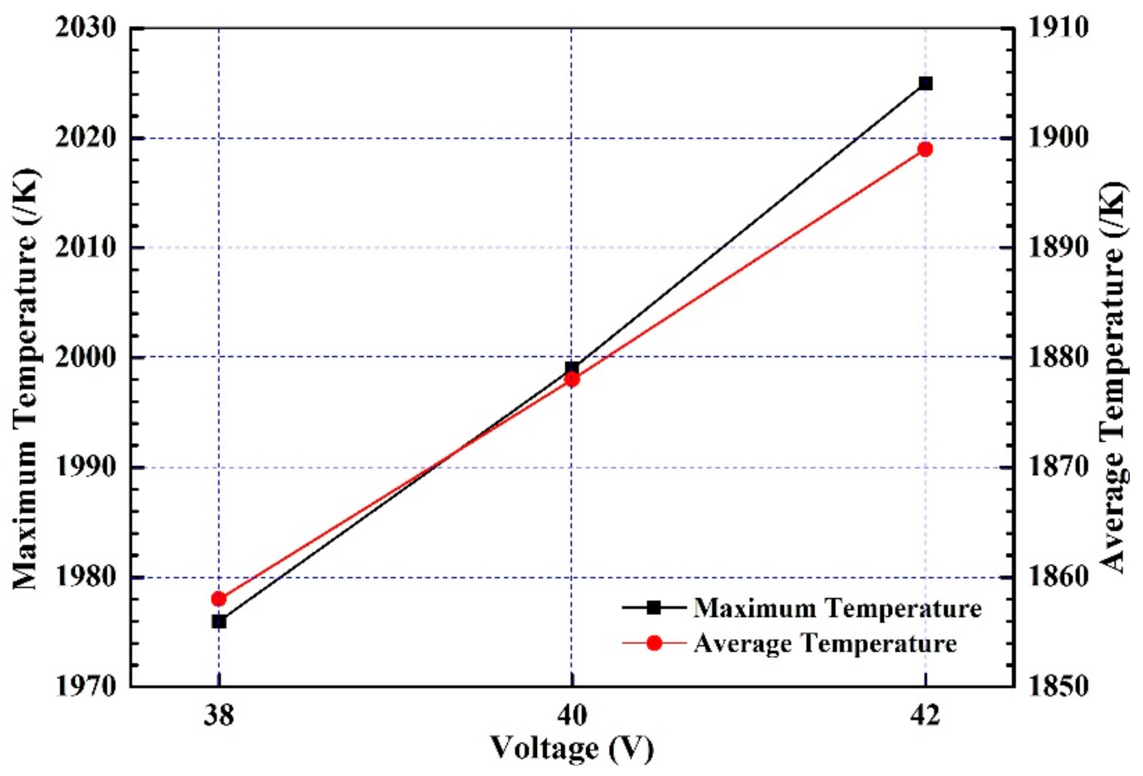
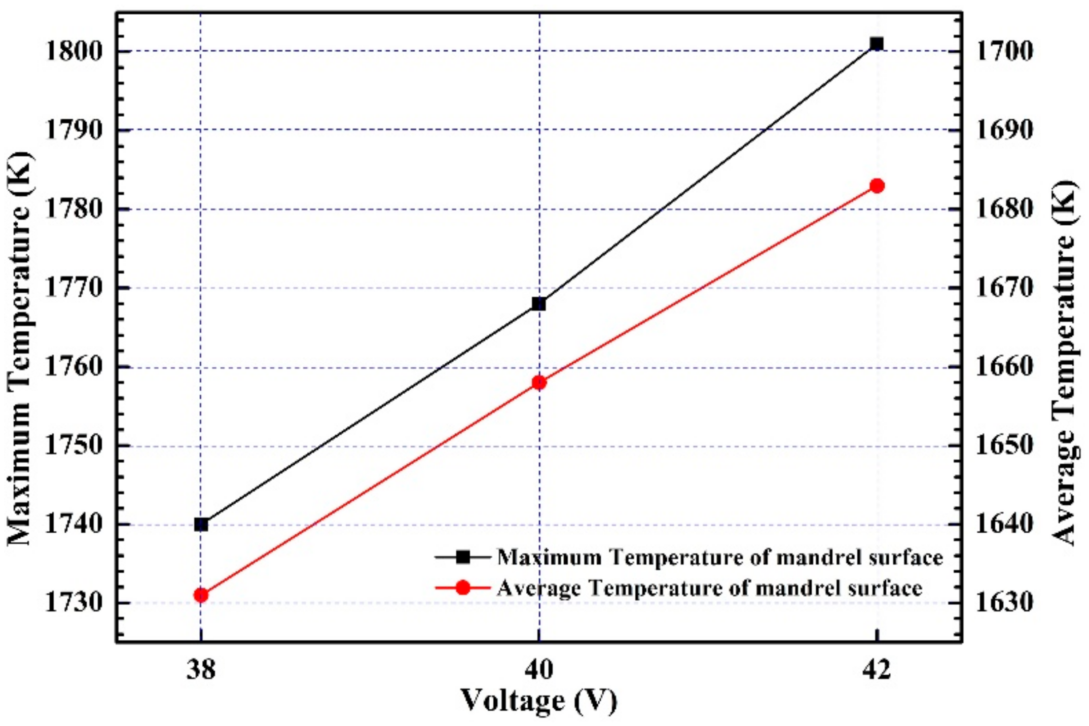
The cross-section (M) passing through slag pool is simulated to study the effect of voltage/power on interface bonding quality. The temperature of mandrel surface increases with more joule heat when the voltage ranges from 38 V to 42 V. The state of the working layer and mandrel changes from separation to connection. In the condition of 40 V, the mandrel and working layer are connected by the fusion layer thickness of 2~4 mm that is helpful to obtain a good interface bonding quality.

References

1. Pellizzari, M.; Molinari, A.; Straffelini, G. Tribological behaviour of hot rolling rolls. Wear 2005, 259, 1281–1289. [Google Scholar] [CrossRef]
2. Pellizzari, M.; Cescato, D.; Flora, M.G.D. Hot friction and wear behaviour of high speed steel and high chromium iron for rolls. Wear 2009, 267, 467–475. [Google Scholar] [CrossRef]
3. Luan, Y.; Song, N.; Bai, Y.; Kang, X.; Li, D. Effect of solidification rate on the morphology and distribution of eutectic carbides in centrifugal casting high-speed steel rolls. J. Mater. Process. Technol. 2010, 210, 536–541. [Google Scholar] [CrossRef]
4. Zhang, T.; Wang, Q.; Song, X.; Fu, H. Effect of electromagnetic centrifugal casting on solidification microstructure of cast high speed steel roll. Materialwiss. Werkstofftech. 2011, 42, 557–561. [Google Scholar] [CrossRef]
5. Hashimoto, M.; Otomo, S.; Yoshida, K.; Kimura, K.; Kurahashi, R.; Kawakami, T.; Kouga, T. Development of high-performance roll by continuous pouring process for cladding. ISIJ Int. 1992, 32, 1202–1210. [Google Scholar] [CrossRef]
6. Medovar, B.I.; Medovar, L.B.; Chemets, A.V.; Shabanov, V.B.; Sviridov, O.V. Ukrain ESS LM HSS Rolls for Hot Strip Mills. Iron and Steel Society. In Proceedings of the 42nd Mechanical Working and Steel Processing Conference, Toronto, ON, Canada, 22–25 October 2000; pp. 647–653. [Google Scholar]
7. Oda, N.; Nozaki, Y.; Honda, R.; Ohata, T. Centrifugally Cast Composite Roll for Hot Rolling and Its Production Method. U.S. Patent 9757779 B2, 12 September 2017. [Google Scholar]
8. Fu, H.G.; Xiao, Q.; Xing, J. Manufacture of centrifugal cast high speed steel rolls for wire rod mills. Ironmak. Steelmak. 2004, 31, 389–392. [Google Scholar] [CrossRef]
9. Hashimoto, M.; Tanaka, T.; Inoue, T.; Yamashita, M.; Kurahashi, R.; Terakado, R. Development of cold rolling mill rolls of high speed steel type by using continuous pouring process for cladding. ISIJ Int. 2002, 42, 982–989. [Google Scholar] [CrossRef]
10. Cao, Y.L.; Jiang, Z.H.; Dong, Y.W.; Deng, X.; Medovar, L.; Stovpchenko, G. Research on the bimetallic composite roll produced by an improved electroslag cladding method: mathematical simulation of the power supply circuits. ISIJ Int. 2018. [Google Scholar] [CrossRef]
11. Dong, Y.W.; Hou, Z.H.; Jiang, Z.H.; Cao, H.B.; Feng, Q.L.; Cao, Y.L. Study of a single-power two-circuit esr process with current-carrying mold: mathematical simulation of the process and experimental verification. Metall. Mater. Trans. B 2018, 49, 249–360. [Google Scholar] [CrossRef]
12. Takeuchi, E.; Zeze, M.; Tanaka, H.; Harada, H.; Mizoguchi, S. Novel continuous casting process for clad steel slabs with level dc magnetic field. Ironmak. Steelmak. 1997, 24, 257–263. [Google Scholar]
13. Sano, Y.; Hattori, T.; Haga, M. Characteristics of high-carbon high speed steel rolls for hot strip mill. ISIJ Int. 1992, 32, 1194–1201. [Google Scholar] [CrossRef]
14. Rao, L.; Wang, S.J.; Zhao, J.H.; Geng, M.P.; Ding, G. Experimental and simulation studies on fabricating GCr15/40Cr bimetallic compound rollers using electroslag surfacing with liquid metal method. Iron Steel Res. Int. 2014, 21, 869–877. [Google Scholar] [CrossRef]
15. Yanke, J.; Fezi, K.; Trice, R.; Krane, M.J.M. Simulation of slag-skin formation in electroslag remelting using a volume-of-fluid method. Numer. Heat Transf. A 2015, 67, 268–292. [Google Scholar] [CrossRef]
16. Fluent 14.5 User’s Guide; Fluent Inc.: Pittsburgh, PA, USA, 2012.
17. Karimi-Sibaki, E.; Kharicha, A.; Bohacek, J.; Wu, M.H.; Ludwing, A. A dynamic mesh-based approach to model melting and shape of an ESR electrode. Metall. Mater. Trans. B 2015, 46, 2049–2061. [Google Scholar] [CrossRef]
18. Kharicha, A.; Ludwig, A.; Wu, M.H. On melting of electrodes during electro-slag remelting. ISIJ Int. 2014, 54, 1621–1628. [Google Scholar] [CrossRef]
19. Song, H.; Ida, N. An eddy current constraint formulation for 3D electromagnetic field calculations. IEEE Trans. Magn. 1991, 27, 4012–4015. [Google Scholar] [CrossRef]
20. Kharicha, A.; Schütenhöer, W.; Ludwig, A.; Tanzer, R. Multiphase modelling of the slag region in ESR Process. In Proceedings of the 2007 International Symposium on Liquid Metal Processing and Casting, Nancy, France, 20–23 September 2007; pp. 107–116. [Google Scholar]
21. Kharicha, A.; Schütenhöer, W.; Ludwig, A.; Reiter, G. Influence of the slag/pool interface on the solidification in an electro-slag remelting process. Mater. Sci. Forum 2010, 649, 229–236. [Google Scholar] [CrossRef]
22. Jardy, A.; Ablitzer, D.; Wadier, J.F. Magnetohydronamic and thermal behavior of electroslag remelting slags. Metall. Mater. Trans. B 1991, 22, 111–120. [Google Scholar] [CrossRef]
23. Dong, Y.W.; Jiang, Z.H.; Cao, Y.L.; Hou, D.; Liang, L.K.; Duan, J.C. Effective thermal conductivity of slag crust for ESR slag. ISIJ Int. 2015, 55, 904–906. [Google Scholar] [CrossRef]
24. Yu, J.; Jiang, Z.H.; Liu, F.B.; Chen, K.; Li, H.B.; Geng, X. Effects of metal droplets on electromagnetic field, fluid flow and temperature field in electroslag remelting process. ISIJ Int. 2017, 57, 1205–1212. [Google Scholar] [CrossRef]
Figure 1. Schematic diagram of an electroslag remelting cladding (ESRC) device. 1-electrical source, 2-electrode, 3-mandrel, 4-liquid slag, 5-current carrying mold, 6-melting steel, 7-working layer, 8-fusion layer, 9-insulation layer; 10-based plate; 11-pulling device.
Metals 08 00504 g001
Figure 2. Geometric model of ESRC: (a) zone and size; (b) boundaries; (c) no movement; (d) movement.
Metals 08 00504 g002aMetals 08 00504 g002b
Figure 3. Schematic diagram of the calculation process.
Metals 08 00504 g003
Figure 4. Contours of the parameters in the slag bath: (a) Voltage; (b) current density; (c) joule heat, (d) magnetic flux density; (e) Lorentz force.
Metals 08 00504 g004aMetals 08 00504 g004b
Figure 5. Contour of parameter in the slag pool: (a) velocity magnitude; (b) temperature field; (c) phase of slag.
Metals 08 00504 g005
Figure 6. Phase of slag at different times: (a) 120 s; (b) 720 s; (c) 1320 s; (d) 1920 s; (e) 2520 s.
Metals 08 00504 g006
Figure 7. Temperature of depth into the mandrel surface on different heating distance with 40 V: (a) 2 mm depth into the mandrel surface; (b) 4 mm depth into the mandrel surface.
Metals 08 00504 g007
Figure 8. Evolution of the maximum current density and joule heat density of the slag pool.
Metals 08 00504 g008
Figure 9. Evolution of the maximum and average temperature of the slag pool with different voltage.
Metals 08 00504 g009
Figure 10. Evolution of the maximum and average temperature of the mandrel surface with different voltage at steady state.
Metals 08 00504 g010
Figure 11. Temperature of points on the cross-section (M) at monitoring points with different voltage: (a) 2 mm, 270 mm; (b) 4 mm, 270 mm.
Metals 08 00504 g011