Accurate Prediction of the Weld Bead Characteristic in Laser Keyhole Welding Based on the Stochastic Kriging Model


1
The State Key Laboratory of Digital Manufacturing Equipment and Technology, School of Mechanical Science and Engineering, Huazhong University of Science & Technology, Wuhan 430074, China
2
School of Aerospace Engineering, Huazhong University of Science & Technology, Wuhan 430074, China
3
George W. Woodruff School of Mechanical Engineering, Georgia Institute of Technology, Atlanta, GA 30332, USA
*
Author to whom correspondence should be addressed.
Metals 2018, 8(7), 486; https://doi.org/10.3390/met8070486
Submission received: 25 May 2018
/
Revised: 17 June 2018
/
Accepted: 18 June 2018
/
Published: 25 June 2018
(This article belongs to the Special Issue Laser Welding)
Abstract
:As an important index of weld quality, the weld bead geometry is closely related to the welding process parameters (WPP). Therefore, it is crucial to establish the relationships between the WPP and weld bead shape to serve as an indicator of the weld quality. However, it is difficult to predict the weld bead shape accurately due to uncertainty. In this paper, laser keyhole welding (LKW) experiments are conducted on 2205 stainless steel at sample points generated by the optimal Latin hypercube sampling (OLHS). Then the relationships between WPP and weld width (WW) are constructed using stochastic kriging model (SKM), considering the randomness of the welding process. To verify the effectiveness of the SKM, two validation approaches, the additional experiments validation and k-fold cross-validation, are used to compare the prediction performance of SKM and the traditional kriging model. SKM is superior to the kriging model at the whole five additional test points with smaller relative error. As to k-fold cross-validation, SKM provides a smaller root mean square error at four in five groups of the data. In addition, SKM can provide the variations of the entire weld bead shape. Overall, the SKM is very prominent in predicting the weld bead shape, considering fluctuations of WPP.
1. Introduction
With the obvious advantages of high efficiency, a narrow heat-affected zone, and small distortion, laser keyhole welding (LKW) has been widely applied in aerospace, aviation, automobile, shipbuilding, and other fields. As intelligent manufacturing develops, accurate predicting of weld bead is becoming crucial to accomplishing industrial automation [1,2]. Therefore, it is necessary to establish the relationships between the laser keyhole welding process parameters (WPP) and weld bead geometry to predict the weld bead quality [3,4,5]. However, the relationship between the WPP and the weld bead is highly nonlinear [6]. The traditional methods of determining process parameters are based on the experience and manual, but the process is difficult to quantify, and the quality of the parameters depends largely on the ability of the engineers [7]. An effective way is to describe the relationships between process parameters and weld bead using the approximate model, which is also called the surrogate model. Gunaraj et al. [8] applied a response surface methodology (RSM) to devise a four-factor five-level central composite rotatable design matrix to fabricate pipes of different specifications in submerged arc welding. Nagesh et al. [9] explored the connection between the shielded metal-arc welding process parameters and the characteristics of the welding bead and penetration utilizing artificial neural networks model. Srivastava et al. [10] employed polynomial response surface (PRS) model to study how the gas metal arc WPP influenced welding quality. Samantaray et al. [11] selected six process parameters and virtual values of two sensor signals to construct six distinguished types of radial basis function network models. Zhou et al. [12] put forward an ensemble of surrogate models to optimize the laser keyhole WPP of stainless steel 316 L.
However, the aforementioned studies assume that the process parameters are stable during the welding process, which is not consistent with practical engineering application scenarios. In the real continuous LKW process, certain parameters fluctuations are inevitable, which will lead to the instability of welding width. Therefore, selecting certain cross sections to represent the entire weld bead’s characteristics is unreliable. The groundbreaking article of Ankenman et al. [13] expanded kriging to include stochastic kriging by classifying the uncertainties in stochastic simulations as extrinsic and intrinsic uncertainty. Chen et al. [14] studied the effect of Common Random Numbers (CRN) on the performance of stochastic kriging predictions, indicating that the introduction of CRN was not conducive to prediction, but better gradient parameter estimation was obtained. The current research on stochastic kriging mainly focuses on theoretical development [15,16,17], while practical engineering applications are rare. In this paper, the SKM is used to predict weld width in LKW by considering the fluctuations of the welding process. Firstly, the experimental sample points are generated using optimal Latin hypercube sampling (OLHS). The image processing techniques are used to extract weld bead features from the specimens. Then two validation methods are used to compare the prediction performance of stochastic kriging and kriging.
The structure of the rest of the paper is as follows. In Section 2, the LKW experimental platform and the experimental process are described in detail. The general framework of the proposed approach and the construction process of SKM are introduced in Section 3. In Section 4, data processing and the evaluation of the predictive performance of the SKM are presented. Section 5 provides the conclusion.
2. Laser Keyhole Welding Procedure
2.1. Problem Definition
According to lots of theoretical research and engineering experience, the weld width largely depends on process parameters such as laser power, welding speed, laser focal position, gap width and shielding gas [18,19]. In this work, three main process parameters (i.e., laser power, welding speed, and focal position) are selected. Low laser power and high welding speed will make the molten pool too small, resulting in incomplete welding and a poor welding formation. On the other hand, excessively high laser power and a low welding speed can cause sag geometry, which will increase the deformation of the weldment and decrease mechanical properties of the weld bead. When the laser focal position is too large, the power density on the workpiece surface is too low to melt required levels of material. According to engineering experience and our previous researches [2,20,21,22], the WPP are selected as follows:
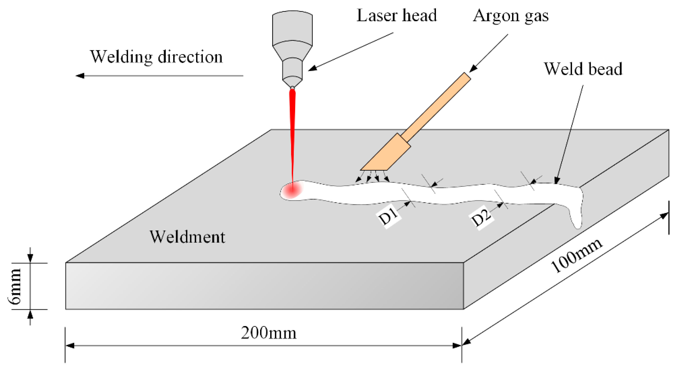
Figure 1 depicts the LKW process. As mentioned earlier, the weld width may fluctuate along the welding direction because of changes of the process parameters. and are the different values of weld width under the same process parameters.
2.2. Materials
With the characteristics of high strength, good impact toughness and good stress corrosion resistance, the 2205 stainless steel was selected as the experimental material. Its chemical composition is shown in Table 1 [23]. The size of the steel sample used in this experiment was . To avoid the influence of the oxide film and oil stain, the sample surface was pretreated with organic solvent acetone.
2.3. Laser Keyhole Welding Process
The experimental setup used for LKW is shown in Figure 2. The laser generation device is IPG YLR-4000 (IPG Photonics Corp., Boston, MA, USA). The laser with a wavelength of passes through the optical fiber to the laser head mounted on the ABB IRB4400 robot. The beam parameter product is . To prevent oxidation during the welding process, the weld bead is protected with argon gas with a flow rate of . Furthermore, the laser power is set through the operation panel of the laser generation device, and the welding path, the welding speed, and the focus point can be controlled by setting the parameters of the welding robot.
3. The Proposed Approach
3.1. General Framework
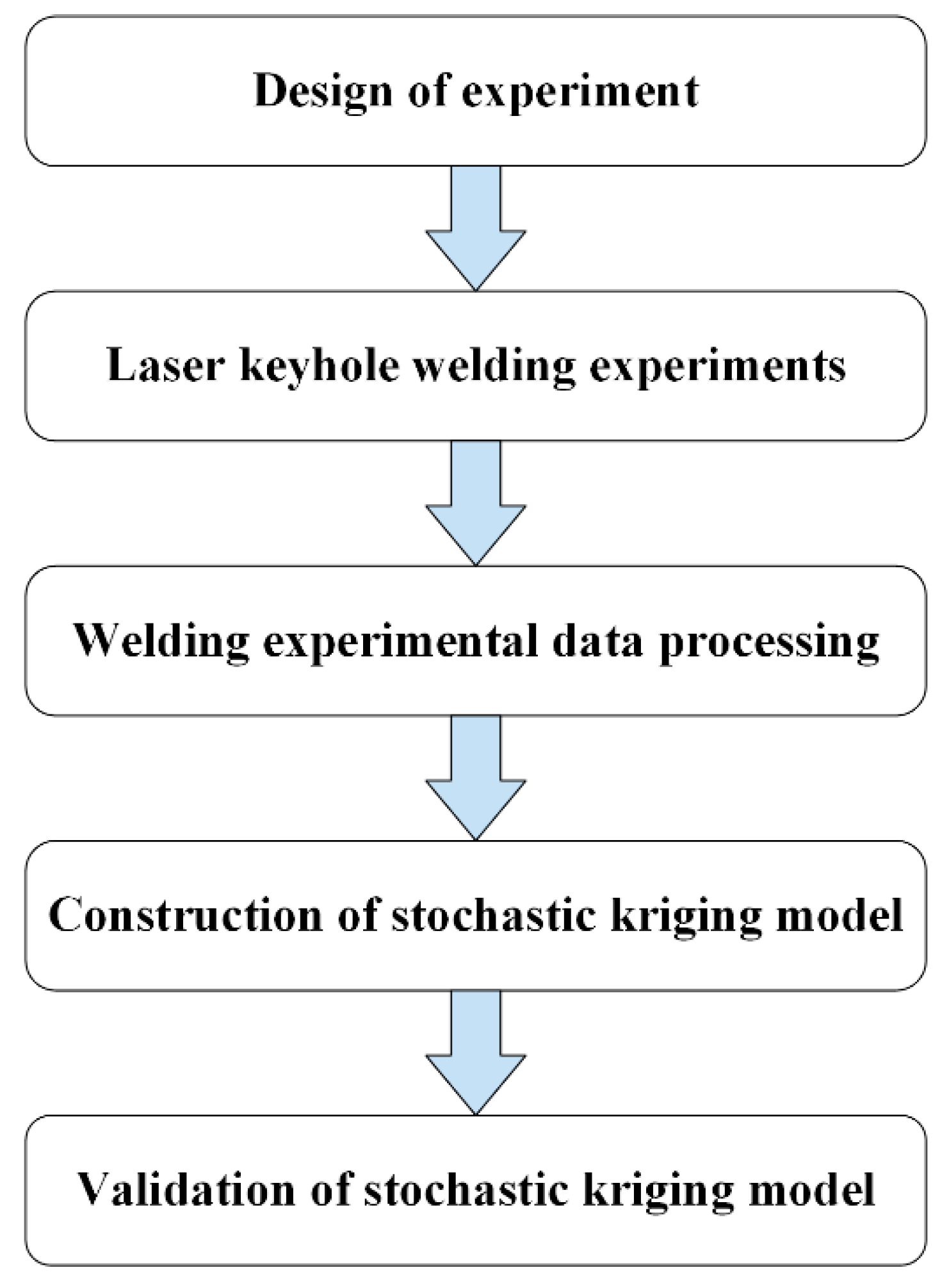
Figure 3 shows the general framework of the proposed approach. The first step consists of design of experiment (DOE) and LKW experiments. The second step is to obtain the mean and variance of weld width and then to construct SKM through these data. The last step is to validate SKM. In this step, additional welding experiments and cross-validation are adopted to compare the weld width prediction accuracies between kriging and SKM.
3.2. Theory of Stochastic Kriging
Deterministic computer experiments do not take into account the noise and errors of the simulation process [24]. Stochastic kriging is an extension of kriging metamodel by considering the uncertainty of the simulation. For the n-dimensional input point , response of stochastic kriging on simulation replication is
where indicates the response of the kriging model without simulated errors at the input point . and represent the corresponding dimensional vectors. is a second-order stationary Gaussian random field with mean zero. denotes the simulation error at replication . According to classic literature on stochastic kriging [13], we call and the extrinsic and intrinsic uncertainty, respectively.
The experimental design of stochastic kriging includes the position of the sample point and the corresponding independent number of replication , which constitutes the data pair . The sample mean at design point is
Let matrix record the intrinsic uncertainty correlation with entry
According to the previous assumption about , can be simplified to a k-dimensional diagonal matrix with
Assume that extrinsic uncertainties possess covariance, which is used to express the spatial correlation between any two points and . The covariance is
where can be explicated as the process variance, and stands for correlation model that is determined by spatial distance .
Define a matrix to express the extrinsic spatial correlation between every two design points, whose element is . Similarly, vector is created to connect the point of interest with design point . Specifically, they are
and
Stochastic kriging obtains the unbiased predicted value at point while minimizing the mean squared error (MSE) for predicting. The expression of is
and the corresponding MSE of is
where and .
In practice, stochastic parameters need to be estimated based on maximum likelihood estimation. By substituting the parameters into Equations (9) and (10), the predicted value and MSE will be obtained.
4. Result and Discussion
4.1. Design of Experiment
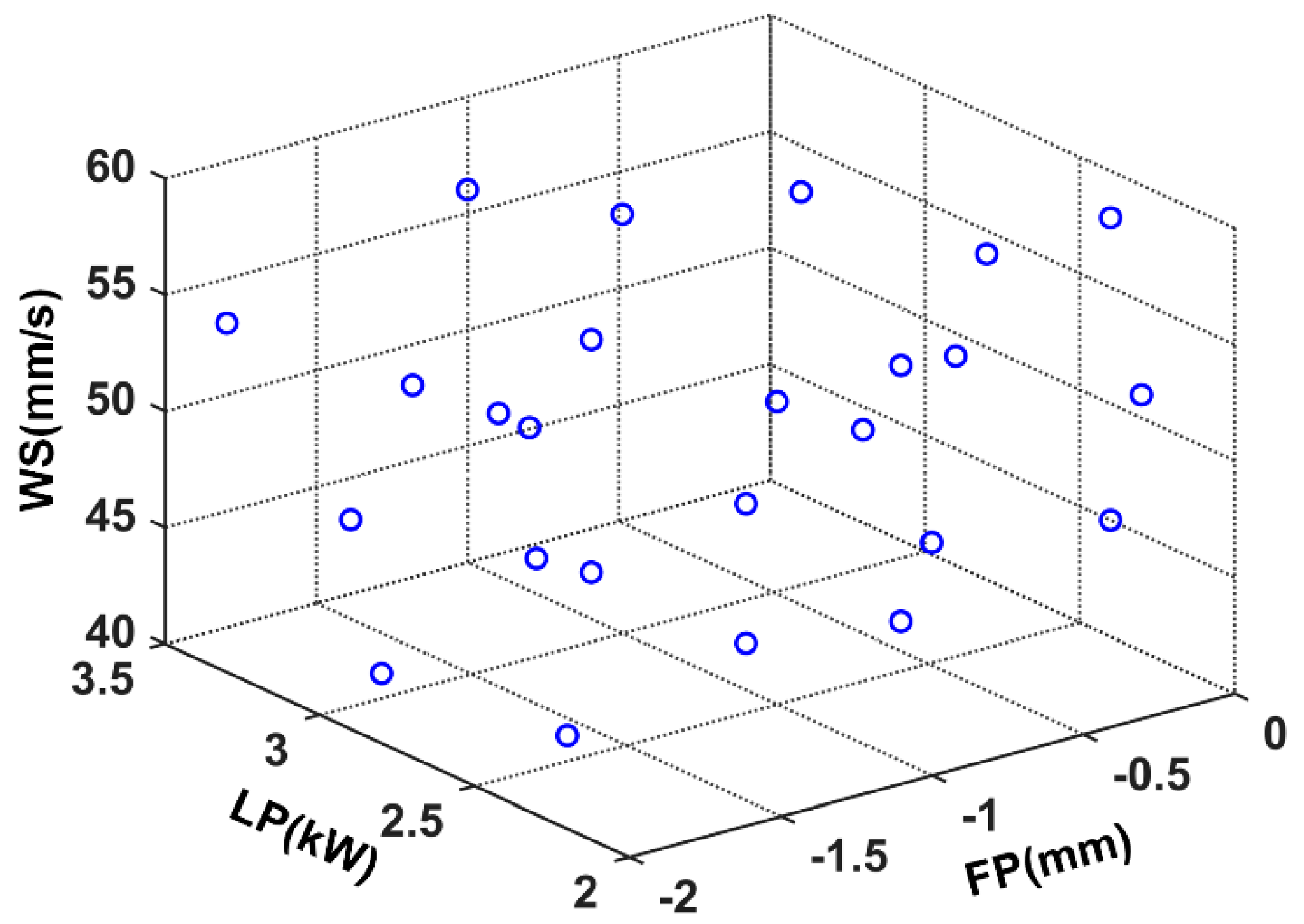
There have been many DOE methods that can fill the experimental design space, such as orthogonal design (UD) [25], center composite design (CCD) [26], and optimal Latin hypercube sampling (OLHS) [27]. OLHS is an improved Latin hypercube sampling (LHS) which evaluates the maximum and minimum distances of points in the search space through a random evolution algorithm to obtain spatially filled sampling points. In this paper, OLHS was used. According to the description in Section 2.1, the laser power, welding speed, and focal position were selected and 25 sample points were generated. The spatial distribution of the generated sample points is shown in Figure 4. The weld width of the corresponding weldments under different process parameters are shown in Table 2.
4.2. Data Processing
4.2.1. Weld Bead Scanning
After obtaining the LKW experimental sample, the next challenge is how to obtain the weld width. In this work, the entire weld width was chosen to be analyzed rather than a certain cross section. The weldment surface was scanned using a scanner and then the width information was extracted from the captured image. The scanner is a product of Shanghai Microtek Trade Co., Ltd., Shanghai, China, whose model is MRS-2400A48U. A series of images with a pixel density of 600 dpi were collected. Table 3 illustrates part of weld bead and the corresponding image processing results of No. 1 to No. 5 specimens.
4.2.2. Image Processing and Feature Extracting
Welding defects are likely to occur at the beginning and end of welding, and the appearance of the weld bead will fluctuate considerably. To improve the prediction accuracy of the weld width, only the stable part of the weld bead was selected for analysis in this work. Perpendicular to the welding direction, the Matlab program (R2017a, MathWorks Inc., Natick, MA, USA) was applied to extract the number of pixels () between the highest and lowest white pixels. The scanned image has a pixel density () of 600 dpi, so the data obtained here can be converted into length in mm according to the following equation
where represents the unit conversion between inches and millimeters, equal to 25.4. In addition, indicates weld width.
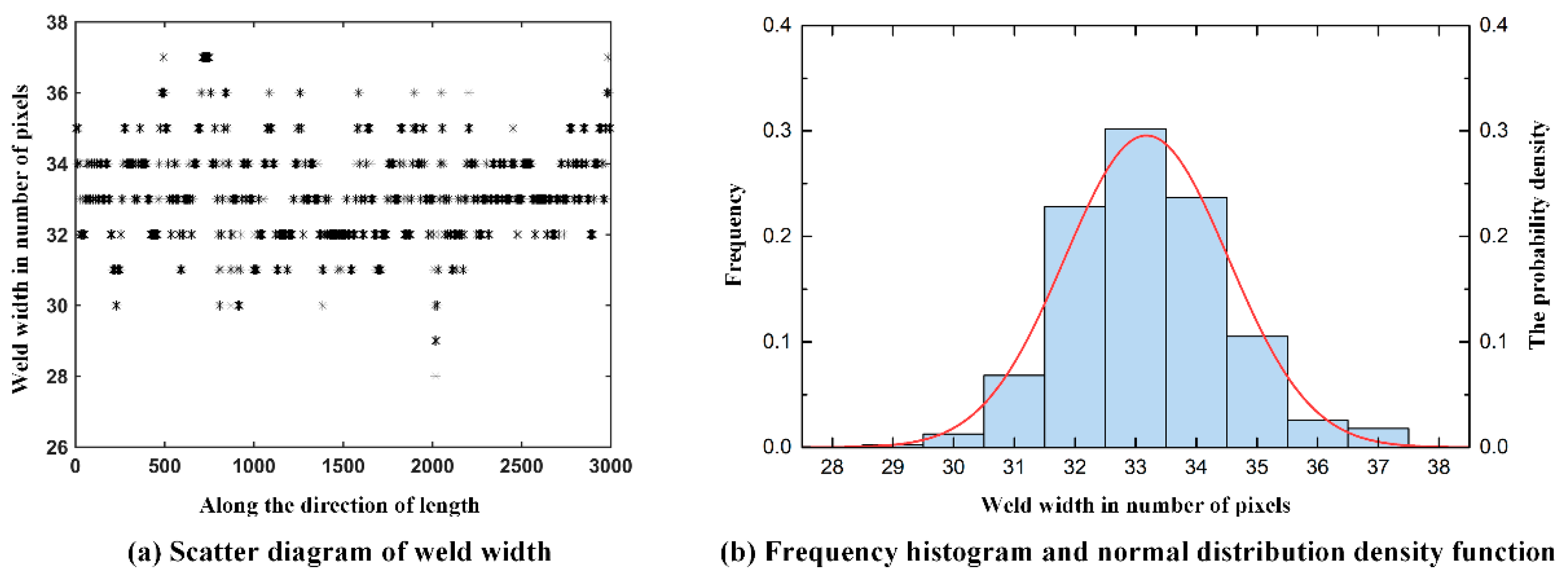
For each weld bead, a set of discretized data of weld width is obtained. The minimum resolution of the scanned image is a pixel, corresponding to the weld width of 0.0423 mm according to Equation (11). For example, the scatter plot of discrete weld width of No. 1 weld bead along the length direction is shown in Figure 5a. Then the probability of weld width is calculated, and the maximum likelihood estimation method is adopted to obtain the mean and variance. A frequency histogram and fitting normal distribution density function of the No. 1 weld bead are shown in Figure 5b. The mean and variance of the normal distribution fitting will be used to construct the SKM.
4.3. Prediction Performance of the Stochastic Kriging Model
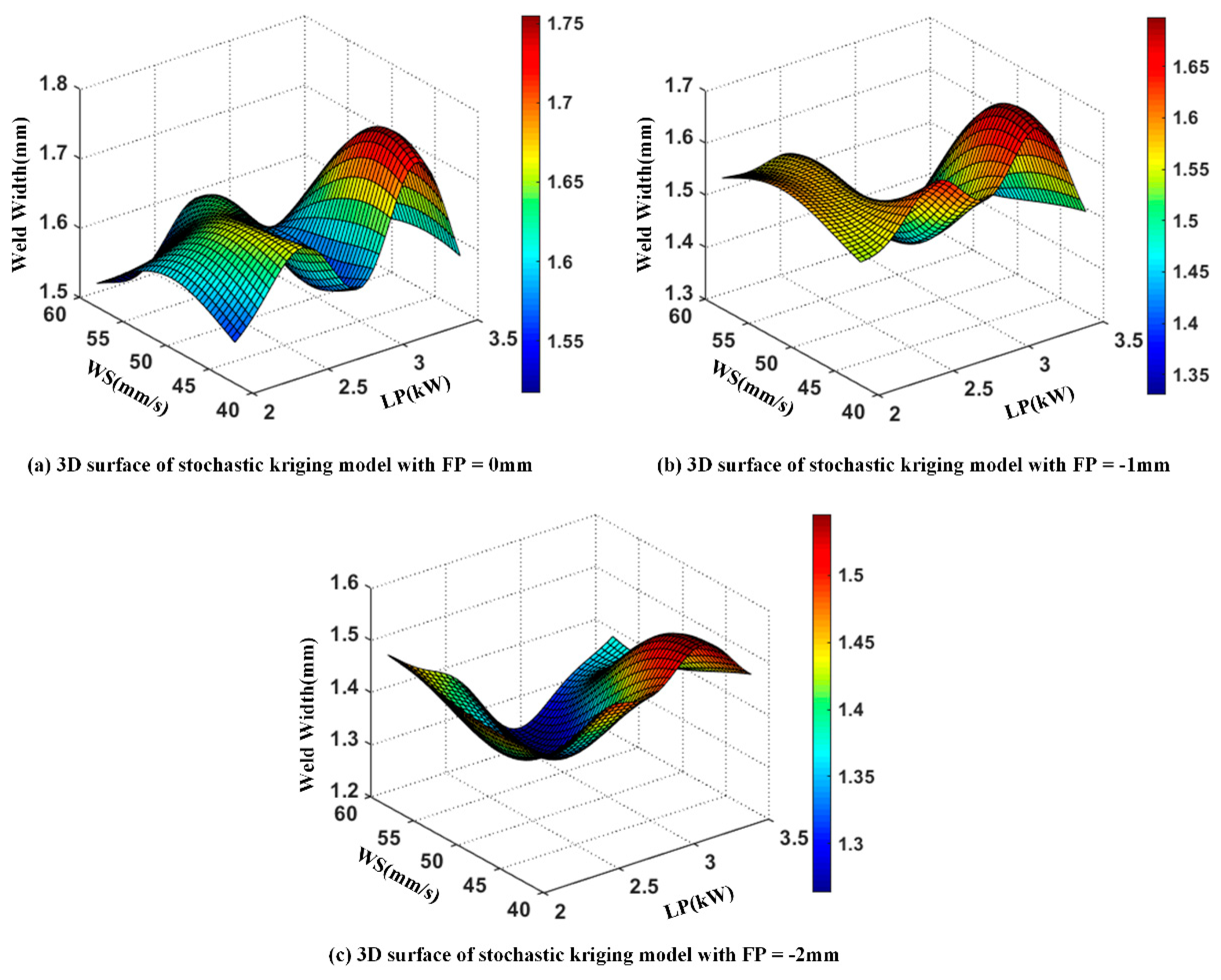
The Matlab program was used to construct SKM. The regression model is with polynomials of order 0. The parameters (i.e.,) that need to be estimated correspond to (). According to the difference of focal position, the three-dimensional surface of the SKM is shown in Figure 6.
To verify the effectiveness of the SKM, the kriging model was also constructed with the same sample points, and the 3D surface of the kriging model is shown in Figure 7. To ensure a fair comparison, the estimated parameters of the two models have the same initial value and range. The range of parameters is 0.01 to 20, and their initial value is 0.1. The parameter estimates (i.e., ) of kriging model correspond to ().
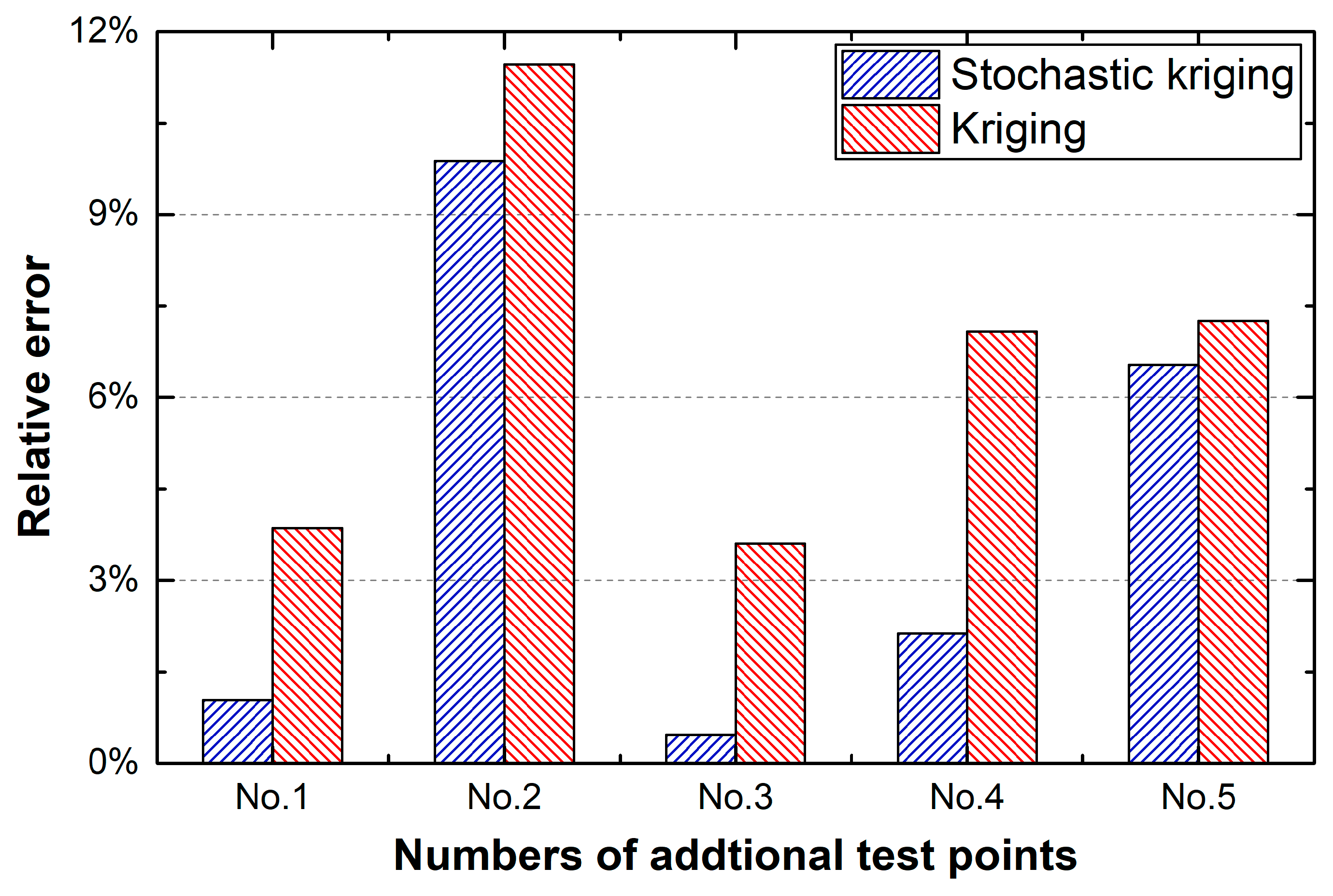
Two validation methods are introduced to compare the prediction performance of the weld width between the SKM and kriging model. First, 5 additional test points were generated randomly based on the same experimental and data processing methods to obtain the corresponding experimental values. The actual values of weld width at the test points are shown in Table 4. Figure 8 plots the relative prediction errors of the kriging and the SKMs. Both of the models have the largest prediction bias at No. 2 point, which are 9.88% and 11.46% respectively. The minimum prediction deviation appears at No. 3 point, corresponding to 0.47% and 3.60%. Obviously, the prediction accuracies of the SKM and kriging model have the same trend, and the SKM performs better due to considering the input uncertainty.
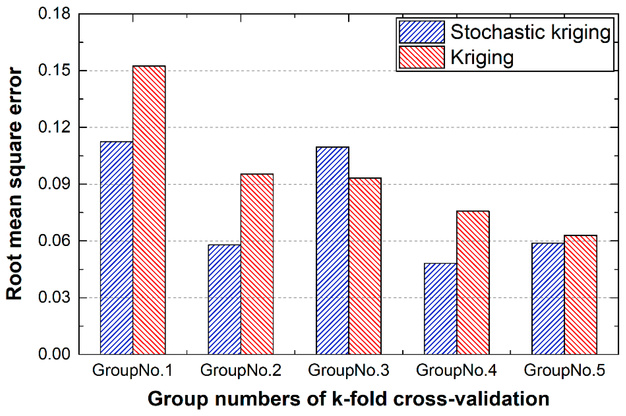
Furthermore, k-fold cross-validation is applied to further verify the prediction performance of SKM. k-fold cross-validation can make full use of existing data as both training and verification points, and its mathematical form is extremely simple [28]. The specific procedure to get the variance of k-fold cross-validation is as follows:
Step 1: Randomly divide the experimental data set into non-repeating and equal-length groups , where is the number of sample points and is the response of .
Step 2: Remove one group from the set , then construct approximate model by using the remaining set .
Step 3: Predict the response values at the removal set Mi by using the model constructed at Step 2, and calculate the root mean square error () by
where is the true response at group , while represents the corresponding approximate model prediction. is the number of data in .
Step 4: Repeat Step 2 to Step 3 times, until the whole data set is considered.
In this work, the 25 sample points were randomly divided into five groups, and each of them consists five sample points. The order of groups was , , , , , where the number corresponded to the No. in Table 2. The comparison results between SKM and kriging model are summarized in Figure 9. It is obvious that stochastic kriging provides better prediction performance. To better illustrate the problem and avoid contingency, k-fold cross-validation was repeated several times, and the same conclusion was drawn. All repeated cross-validation shows that SKM has better performance in weld width prediction. Taking Figure 9 as an example, SKM provides smaller RMSE except for the third group.
5. Conclusions
In this work, the SKM has been used to predict the weld width of LKW. Unlike the general data acquisition method, this paper effectively obtains the properties of the whole weld by combining the weld bead scan with the image processing. Based on the estimated mean and variance of the normal distribution fitting of weld width, the SKM was constructed to fit the relationships between the laser power, the welding speed, the focal position and the weld width. Additional experiments and k-fold cross-validation are introduced to compare the prediction performance of weld width between SKM and kriging model. The comparison results indicate that the SKM is feasible and very prominent for predictions of the weld bead shape.
Author Contributions
Data curation, X.R.; Formal analysis, L.S.; Methodology, Q.Z., J.H. and L.C.; Supervision, Q.Z.; Validation, L.C.; Writing—original draft, X.R. and L.C.; Writing—review & editing, Q.Z. and L.C.
Funding
This research received no external funding.
Acknowledgments
This research has been supported by National Natural Science Foundation of China (NSFC) under Grant No. 51505182.
Conflicts of Interest
The authors declare no conflict of interest.
Nomenclature
| DOE | Design of experiment |
| FP | Focal position |
| LKW | Laser keyhole welding |
| LP | Laser power |
| OLHS | Optimal Latin hypercube sampling |
| SKM | Stochastic kriging model |
| WPP | Welding process parameters |
| WS | Welding speed |
| WW | Weld width |
References
- Yuce, C.; Tutar, M.; Karpat, F.; Yavuz, N. The optimization of process parameters and microstructural characterization of fiber laser welded dissimilar HSLA and MART steel joints. Metals 2016, 6, 245. [Google Scholar] [CrossRef]
- Cao, L.; Shao, X.; Jiang, P.; Zhou, Q.; Rong, Y.; Geng, S.; Mi, G. Effects of welding speed on microstructure and mechanical property of fiber laser welded dissimilar butt joints between AISI316L and EH36. Metals 2017, 7, 270. [Google Scholar] [CrossRef]
- Murugan, N.; Gunaraj, V. Prediction and control of weld bead geometry and shape relationships in submerged arc welding of pipes. J. Mater. Process. Technol. 2005, 168, 478–487. [Google Scholar] [CrossRef]
- Ridha Mohammed, G.; Ishak, M.; Ahmad, S.N.A.S.; Abdulhadi, H.A. Fiber laser welding of dissimilar 2205/304 stainless steel plates. Metals 2017, 7, 546. [Google Scholar] [CrossRef]
- Loginova, I.; Khalil, A.; Pozdniakov, A.; Solonin, A.; Zolotorevskiy, V. Effect of pulse laser welding parameters and filler metal on microstructure and mechanical properties of Al-4.7 Mg-0.32 Mn-0.21 Sc-0.1 Zr Alloy. Metals 2017, 7, 564. [Google Scholar] [CrossRef]
- Kim, I.; Son, J.; Kim, I.; Kim, J.; Kim, O. A study on relationship between process variables and bead penetration for robotic CO2 arc welding. J. Mater. Process. Technol. 2003, 136, 139–145. [Google Scholar] [CrossRef]
- Fukuda, S.; Morita, H.; Yamauchi, Y.; Nagasawa, I.; Tsuji, S. Expert system for determining welding condition for a pressure vessel. ISIJ Int. 1990, 30, 150–154. [Google Scholar] [CrossRef]
- Gunaraj, V.; Murugan, N. Application of response surface methodology for predicting weld bead quality in submerged arc welding of pipes. J. Mater. Process. Technol. 1999, 88, 266–275. [Google Scholar] [CrossRef]
- Nagesh, D.; Datta, G. Prediction of weld bead geometry and penetration in shielded metal-arc welding using artificial neural networks. J. Mater. Process. Technol. 2002, 123, 303–312. [Google Scholar] [CrossRef]
- Srivastava, S.; Garg, R. Process parameter optimization of gas metal arc welding on IS: 2062 mild steel using response surface methodology. J. Manuf. Process. 2017, 25, 296–305. [Google Scholar] [CrossRef]
- Pal, S.; Pal, S.K.; Samantaray, A.K. Radial basis function neural network model based prediction of weld plate distortion due to pulsed metal inert gas welding. Sci. Technol. Weld. Join. 2007, 12, 725–731. [Google Scholar] [CrossRef]
- Jiang, P.; Wang, C.; Zhou, Q.; Shao, X.; Shu, L.; Li, X. Optimization of laser welding process parameters of stainless steel 316L using FEM, Kriging and NSGA-II. Adv. Eng. Softw. 2016, 99, 147–160. [Google Scholar] [CrossRef]
- Ankenman, B.; Nelson, B.L.; Staum, J. Stochastic kriging for simulation metamodeling. Oper. Res. 2010, 58, 371–382. [Google Scholar] [CrossRef]
- Chen, X.; Ankenman, B.E.; Nelson, B.L. The effects of common random numbers on stochastic kriging metamodels. ACM Trans. Model. Comput. Simul. (TOMACS) 2012, 22, 7. [Google Scholar] [CrossRef]
- Xie, W.; Nelson, B.; Staum, J. The influence of correlation functions on stochastic kriging metamodels. In Proceedings of the 2010 Winter Simulation Conference, Baltimore, MD, USA, 5–8 December 2010; pp. 1067–1078. [Google Scholar]
- Kamiński, B. A method for the updating of stochastic kriging metamodels. Eur. J. Oper. Res. 2015, 247, 859–866. [Google Scholar] [CrossRef]
- Liu, M.; Staum, J. Stochastic kriging for efficient nested simulation of expected shortfall. J. Risk 2010, 12, 3. [Google Scholar] [CrossRef]
- El-Batahgy, A.-M. Effect of laser welding parameters on fusion zone shape and solidification structure of austenitic stainless steels. Mater. Lett. 1997, 32, 155–163. [Google Scholar] [CrossRef]
- Cicală, E.; Duffet, G.; Andrzejewski, H.; Grevey, D.; Ignat, S. Hot cracking in Al–Mg–Si alloy laser welding-operating parameters and their effects. Mater. Sci. Eng. A 2005, 395, 1–9. [Google Scholar] [CrossRef]
- Cao, L.; Yang, Y.; Jiang, P.; Zhou, Q.; Mi, G.; Gao, Z.; Rong, Y.; Wang, C. Optimization of processing parameters of AISI 316L laser welding influenced by external magnetic field combining RBFNN and GA. Results Phys. 2017, 7, 1329–1338. [Google Scholar] [CrossRef]
- Zhou, Q.; Rong, Y.; Shao, X.; Jiang, P.; Gao, Z.; Cao, L. Optimization of laser brazing onto galvanized steel based on ensemble of metamodels. J. Intell. Manuf. 2016, 1–15. [Google Scholar] [CrossRef]
- Jiang, P.; Cao, L.; Zhou, Q.; Gao, Z.; Rong, Y.; Shao, X. Optimization of welding process parameters by combining Kriging surrogate with particle swarm optimization algorithm. Int. J. Adv. Manuf. Technol. 2016, 86, 2473–2483. [Google Scholar] [CrossRef]
- Michalska, J.; Sozańska, M. Qualitative and quantitative analysis of σ and χ phases in 2205 duplex stainless steel. Mater. Charact. 2006, 56, 355–362. [Google Scholar] [CrossRef]
- Lophaven, S.; Nielsen, H.; Søndergaard, J. DACE-A MATLAB Kriging Toolbox—Version 2.0.(2002); Technical University of Denmark: Lyngby, Denmark, 2002. [Google Scholar]
- Seberry, J. Orthogonal designs. In Orthogonal Designs: Hadamard Matrices, Quadratic Forms and Algebras; Springer: Cham, Switzerland, 2017; pp. 1–5. [Google Scholar]
- Montgomery, D.C.; Runger, G.C.; Hubele, N.F. Engineering Statistics; John Wiley & Sons: Hoboken, NJ, USA, 2009. [Google Scholar]
- Park, J.-S. Optimal Latin-hypercube designs for computer experiments. J. Stat. Plan. Inference 1994, 39, 95–111. [Google Scholar] [CrossRef]
- Refaeilzadeh, P.; Tang, L.; Liu, H. Cross-validation. In Encyclopedia of Database Systems; Springer: Cham, Switzerland, 2009; pp. 532–538. [Google Scholar]
Figure 1.
Schematic diagram of laser keyhole welding process.

Figure 2.
Laser keyhole welding equipment.
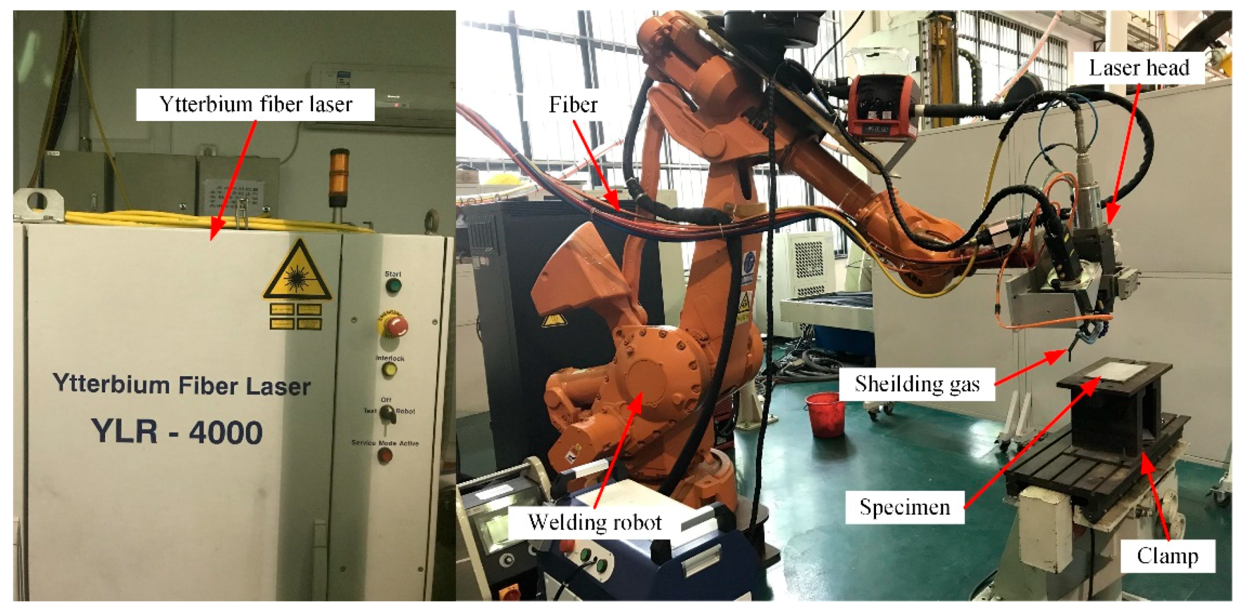
Figure 3.
General framework of the proposed approach.

Figure 4.
Spatial distribution diagram of the generated sample points.

Figure 5.
Discretized data of weld width.

Figure 6.
The stochastic kriging model for weld width prediction.

Figure 7.
The kriging model for weld width prediction.
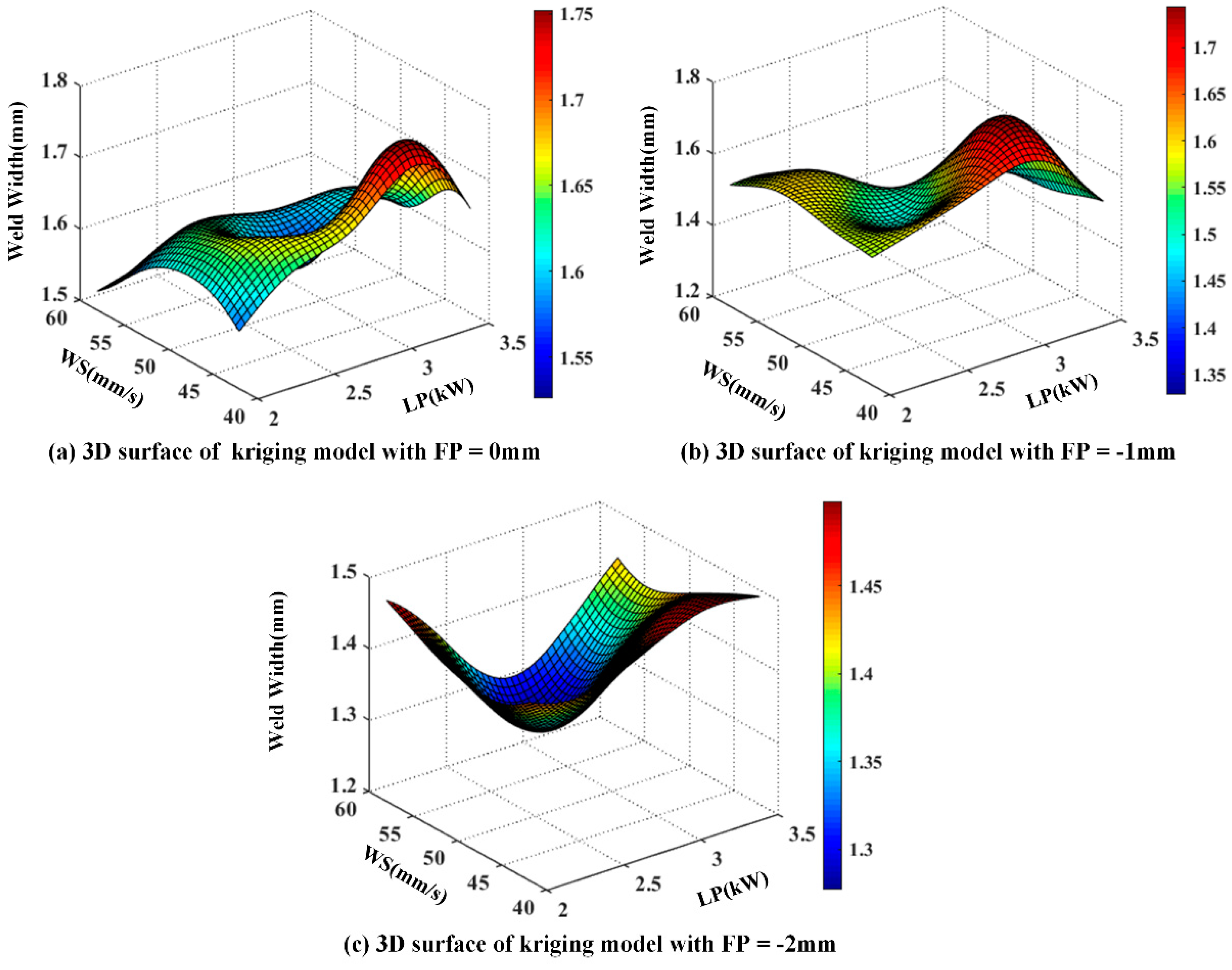
Figure 8.
Relative prediction errors of the stochastic kriging model and the kriging model.

Figure 9.
The comparison of RMSE between stochastic kriging model and kriging model.


Table 1.
Chemical composition of 2205 stainless steel.
| Chemical Elements | C | Cr | Ni | Mo | Mn | Si | P | S | N |
|---|---|---|---|---|---|---|---|---|---|
| Composition (%) | 0.025 | 22.73 | 5.53 | 3.03 | 1.89 | 0.34 | 0.028 | 0.002 | 0.170 |
Table 2.
Weld width under different process parameters.
| No. | FP (mm) | LP (kW) | WS (mm/s) | Weld Width (mm) | Variance (10−6) |
|---|---|---|---|---|---|
| 1 | −2 | 2.2 | 44 | 1.40 | 1.09 |
| 2 | −2 | 2.3 | 51 | 1.35 | 2.1 |
| 3 | −2 | 3.3 | 55 | 1.37 | 1.33 |
| 4 | −2 | 2.8 | 43 | 1.46 | 1.49 |
| 5 | −2 | 2.9 | 49 | 1.37 | 1.50 |
| 6 | −2 | 2.7 | 56 | 1.29 | 0.89 |
| 7 | −1 | 2.0 | 50 | 1.59 | 1.06 |
| 8 | −1 | 2.1 | 46 | 1.56 | 3.54 |
| 9 | −1 | 2.1 | 57 | 1.56 | 1.29 |
| 10 | −1 | 2.5 | 53 | 1.55 | 6.27 |
| 11 | −1 | 2.6 | 48 | 1.50 | 4.82 |
| 12 | −1 | 2.6 | 42 | 1.63 | 2.38 |
| 13 | −1 | 3.0 | 58 | 1.33 | 3.44 |
| 14 | −1 | 3.1 | 42 | 1.67 | 3.20 |
| 15 | −1 | 3.1 | 52 | 1.52 | 2.35 |
| 16 | −1 | 3.3 | 47 | 1.64 | 2.56 |
| 17 | −1 | 3.4 | 47 | 1.55 | 2.32 |
| 18 | −1 | 3.5 | 56 | 1.41 | 2.68 |
| 19 | 0 | 2.3 | 51 | 1.64 | 0.98 |
| 20 | 0 | 2.4 | 45 | 1.66 | 5.16 |
| 21 | 0 | 2.4 | 58 | 1.55 | 2.29 |
| 22 | 0 | 2.8 | 54 | 1.60 | 3.08 |
| 23 | 0 | 2.9 | 49 | 1.57 | 6.77 |
| 24 | 0 | 3.2 | 44 | 1.75 | 3.11 |
| 25 | 0 | 3.4 | 53 | 1.61 | 3.62 |
Table 3.
Weld bead of No. 1 to No. 5 specimens.
| No. | Weld Appearance | Image Processing |
|---|---|---|
| 1 |  |  |
| 2 | 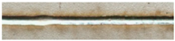 |  |
| 3 | 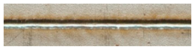 |  |
| 4 | 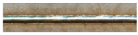 |  |
| 5 | 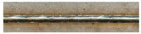 |  |
Table 4.
Weld bead of additional test points.
| No. | FP (mm) | LP (kW) | WS (mm/s) | Weld Width (mm) | Variance (10−6) |
|---|---|---|---|---|---|
| 1 | −2 | 3.2 | 58 | 1.32 | 1.22 |
| 2 | −2 | 3.3 | 42 | 1.69 | 1.71 |
| 3 | −1 | 2.7 | 53 | 1.45 | 4.55 |
| 4 | −1 | 3.0 | 51 | 1.46 | 2.39 |
| 5 | 0 | 2.5 | 55 | 1.74 | 3.29 |
© 2018 by the authors. Licensee MDPI, Basel, Switzerland. This article is an open access article distributed under the terms and conditions of the Creative Commons Attribution (CC BY) license (http://creativecommons.org/licenses/by/4.0/).
Share and Cite
MDPI and ACS Style
Ruan, X.; Zhou, Q.; Shu, L.; Hu, J.; Cao, L. Accurate Prediction of the Weld Bead Characteristic in Laser Keyhole Welding Based on the Stochastic Kriging Model. Metals 2018, 8, 486. https://doi.org/10.3390/met8070486
AMA Style
Ruan X, Zhou Q, Shu L, Hu J, Cao L. Accurate Prediction of the Weld Bead Characteristic in Laser Keyhole Welding Based on the Stochastic Kriging Model. Metals. 2018; 8(7):486. https://doi.org/10.3390/met8070486
Chicago/Turabian StyleRuan, Xiongfeng, Qi Zhou, Leshi Shu, Jiexiang Hu, and Longchao Cao. 2018. "Accurate Prediction of the Weld Bead Characteristic in Laser Keyhole Welding Based on the Stochastic Kriging Model" Metals 8, no. 7: 486. https://doi.org/10.3390/met8070486
Note that from the first issue of 2016, this journal uses article numbers instead of page numbers. See further details here.