
Predicted Fracture Behavior of Shaft Steels with Improved Corrosion Resistance


.JPG)
1
Department of Marine Engineering and Ship Power Systems, Faculty of Maritime Studies Rijeka, University of Rijeka, Rijeka 51000, Croatia
2
Department of Engineering Mechanics, Faculty of Engineering, University of Rijeka, Rijeka 51000, Croatia
*
Author to whom correspondence should be addressed.
Metals 2016, 6(2), 40; https://doi.org/10.3390/met6020040
Submission received: 14 January 2016
/
Revised: 4 February 2016
/
Accepted: 14 February 2016
/
Published: 19 February 2016
Abstract
:One of the crucial steps in the shaft design process is the optimal selection of the material. Two types of shaft steels with improved corrosion resistances, 1.4305 and 1.7225, were investigated experimentally and numerically in this paper in order to determine some of the material characteristics important for material selection in the engineering design process. Ultimate tensile strength and yield strength have been experimentally obtained, proving that steel 1.4305 has higher values of both. In addition, J-integral is numerically determined as a measure of crack driving force for finite element models of standardized fracture specimens (single-edge notched bend and disc compact tension). Obtained J values are plotted versus specimen crack growth size (Δa) for different specimen geometries (a/W). Higher resulting values of J-integral for steel 1.4305 as opposed to 1.7225 can be noted. Results can be useful as a fracture parameter in fracture toughness assessment, although this procedure differs from experimental analysis.
1. Introduction
Material selection is a crucial step in the process of engineering design. Optimal selection of the material can significantly reduce the possibility of failures, along with understanding the nature and stress intensity that occurs in a designed structure. Engineering practices usually distinguishes one or few causes of failure: excessive force and/or temperature-induced elastic deformation, yielding, fatigue, corrosion, creep, etc. Selection of improper materials may have a negative effect on operational lifetime cycle and result in flaw appearance, which can cause structural failure.
A successful material-selection process implies reconciling requirements, such as appropriate strength of a material, sufficient level of rigidity, heat resistance, etc. For structures susceptible to crack growth, it is necessary to ensure that the material has been selected on the basis of fracture mechanics parameters.
Considering shaft design, the fracture mechanics approach must be used in order to account for high stresses and harsh operating conditions. Implementation of the fracture mechanics approach has the benefit of reducing potential failures, such as the fatigue induced fracture presented in a study of marine main engine crankshaft failure [1]. The agitator steel shaft failed due to an inadequate design, which was incapable of withstanding torsional-bending fatigue during operation [2]. The gearbox shaft failure occurred due to high stress concentrations at the corners of the wobbler of the shaft, causing fatigue crack initiation [3]. Improved design and machining practice suggested that this would help to prolong service life of the component. A forklift collapsed due to failure of axle shaft, caused by material inclusions and poor heat treatment [4].
Most of the mentioned failures occurred on steels typically used in the manufacturing of shafts intended for use in harsh environments, where a higher corrosion resistance is necessary. To be able to properly choose a suitable material for such an environment, characterization of a material is essential.
Fracture mechanics parameters that define material resistance to crack propagation are usually determined through experimental investigations of the material under consideration. Fracture behavior is usually estimated using some of the well-established fracture parameters, such as stress intensity factor (K), J-integral, or crack tip opening displacement (CTOD). J-integral is appropriate for quantifying material resistance to crack extension when dealing with ductile fracture of metallic materials, which includes nucleation, growth, and coalescence of voids [5]. For a growing crack, J-integral values can be determined for a range of crack extensions (Δa) and can be presented in the form of the J-resistance curve. This curve is usually obtained experimentally following standardized procedures, but it can be successfully complemented or even substituted by numerical methods, e.g., the finite element (FE) method. Some of the recent articles on this topic include discussion on the accuracy of J-integral obtained by experiments, two-dimensional (2D) FE analysis, three-dimensional (3D) FE analysis, or the Electric Power Research Institute method [6]. J-integral and CTOD are related through plastic constraint factors evaluated using 3D FE analyses of a clamped, single-edge tension specimen [7]. Methodology to evaluate 3D J-integral for finite strain elastic-plastic solid using FE analysis is proposed [8]. Stress intensity factors and T-stress of 3D interface cracks and notches are computed using the scaled boundary FE method [9].
This paper presents a comparison of numerically predicted J-values taken from the measure of crack driving force for two types of steel commonly used in shaft manufacturing, steels 1.4305 and 1.7225. Obtained material data may help designers to find the best solution in appropriate material selection.
2. Materials and Methods
2.1. Considered Materials
The two materials compared are stainless steel 1.4305 (AISI 303) and alloy steel 1.7225 (AISI 4140). Steel 1.4305, commonly named chromium-nickel steel, is a derivative of a common grade stainless steel 1.4301, but with improved machinability. Chromium-molybdenum steel 1.7225 has an excellent strength to weight ratio, is readily machinable, and suitable for forging between 900 and 1200 °C.
The two materials differ substantially with respect to chemical composition (Table 1).
Comparing the composition of steel 1.4305 to standard EN 10088-2:2005, it can be noted that the nickel percentage in the considered steel is just below the standard range (8%–10%), while manganese equals the maximum standard value (2%). As for steel 1.7225, comparing it to standard EN 10083-3:2006, it can be noted that carbon is equal to the maximum standard value (0.45%), while other elements are in standard ranges.
Both steels are widely considered for shafts intended to be used in marine, the petro or chemical industries, or as vehicular components, because both offer improved corrosion resistance, but with 1.4305 having significantly better resistance in a corrosive environment due to its elevated chromium content. Considering the differences in composition and corrosion resistance, it can be concluded that the two materials correspond to somewhat different ranges of specific applications. Steel 1.7225 can be found in bridge crane shafts [10], which are prone to fatigue failure, marine diesel engine crankshafts [11], where a material has to be adequate to severe working conditions, automotive applications [12], where axle shafts are sensitive to improper heat treatment, or in diesel engines of commercial vehicles [13], in which crankshafts need to be machined properly in order to avoid fatigue fractures. Chromium-nickel stainless steels can be found in agitator steel shafts [2] or mixer unit shafts [14], which prone to intergranular stress cracking at weld heat affected zones.
The equipment used to determine the mechanical properties of the materials was a computer-directed, materials testing machine (Zwick/Roell 400 kN, Zwick/Roell, Ulm, Germany) (Figure 1). Specimens were manufactured from rods made of the considered steels. Specimen geometry and uniaxial tensile test procedure were set, according to appropriate American Society for Testing and Materials (ASTM) standard [15]. Experimentally-obtained stress-strain curves are shown in Figure 2, and values of yield strength (σYS) and tensile strength (σTS) of considered materials are given in Table 1.
When dealing with the fracture resistant design of structures, fracture toughness has an importance similar to yield strength when dealing with structure design against plastic deformation. The simple Charpy procedure for impact energy determination can be used to determine the fracture parameters. On the basis of known Charpy V-notch (CVN), impact energy correlation with fracture toughness can be made, e.g., with Roberts-Newton formula, independent of CVN energy range and temperature level [18]:
Some experimental data related to CVN energy is presented in Table 2. Charpy V-notch energy was also experimentally determined [16,17]. Experimentally-obtained results show that steel 1.4305 manifests a higher tensile strength and elongation than steel 1.7225, but CVN energy results show that the steel 1.4305 presents a lower CVN and lower fracture toughness than steel 1.7225, which can be attributed to the state of the as-received materials. Steel 1.7225 was a soft annealed as-received material (containing more percentage of carbon), compared to steel 1.4305, which was annealed and cold drawn (containing a lower percentage of carbon).
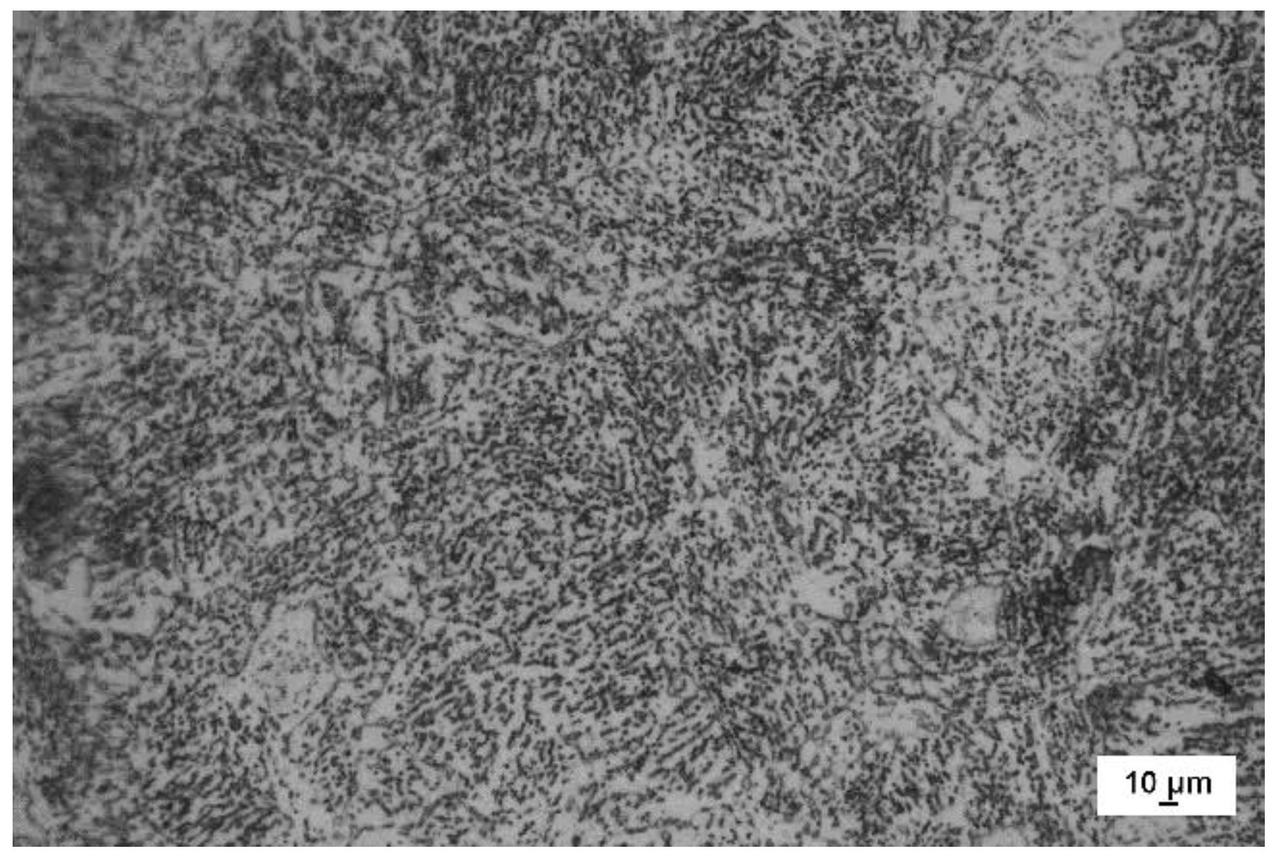
In Figure 3, an optical micrograph of the as-received steel 1.4305 (soft annealed and cold drawn) is presented.
In Figure 4, an optical micrograph of the as-received steel 1.7225 (soft annealed) is presented.
Considering the microstructure of steel 1.4305, it can be said that the basic microstructure of the as-received material is austenite, but there is also a mixture of austenite and ferrite. Considering the microstructure of steel 1.7225, it can be said that its main phase (main structure) consists of a thin pearlitic microstructure, where also a few ferrite and some particles of cementite can be observed.
2.2. Predicted Fracture Behavior of Considered Materials
J-integral is used to numerically predict the fracture behavior of the considered materials. J-integral was introduced by Rice and Cherepanov [19,20], separately, as a path-independent integral, which can be drawn around the tip of a crack and viewed both as an energy release rate parameter and a stress intensity parameter. In a two-dimensional form, it can be written as:
where Ti = σijnj are components of the traction vector, ui are the displacement vector components, and ds is an incremental length along the arbitrary contour path Γ enclosing the crack tip.
In order to predict fracture behavior of steels 1.4305 and 1.7225, an experimental single specimen test method [15] following an elastic unloading compliance technique was numerically simulated. This test method uses measured crack mouth opening displacement to estimate the growing crack size. Resulting J-integral values can be taken as a fracture toughness parameter and plotted versus crack extension. The first step of the numerical procedure is to conduct a structural stress analysis.
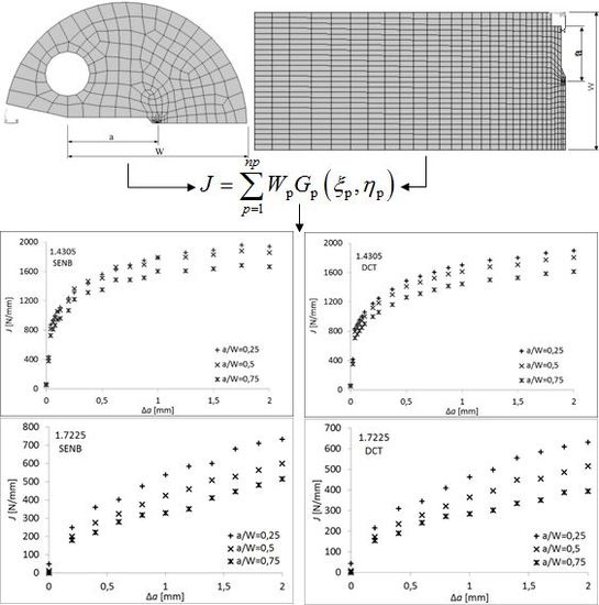
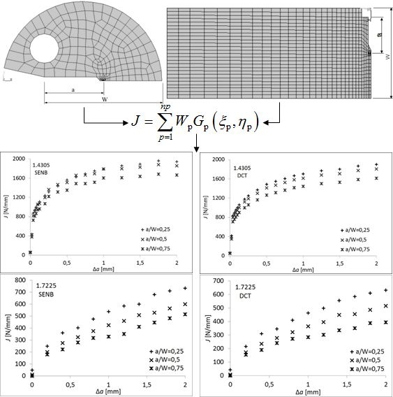
According to the appropriate ASTM standard [15], 2D FE models of the two types of specimens, single edge notched bend (SENB), and disc compact tensile (DCT), are defined and initial a/W (W = 50 mm) ratios of 0.25, 0.5 and 0.75 are taken (Figure 5). The material behavior is considered to be a multilinear isotropic hardening type. FE models of specimens are meshed with 8-node isoparamateric quadrilateral elements. The mesh is refined around the crack tip in order to capture high deformation gradients in the regions where yielding occurs. To simulate compliance procedures of single specimen test method, quasi-static load was imposed on specimen. Only half of the specimen needs to be modeled due to their symmetry. The node releasing technique was used to simulate crack propagation.
FE stress analysis results taken from the integration points of finite elements surrounding the crack tip were used to evaluate J-integral values using the following equation [21]:
where Wp is the Gauss weighting factor, np is the number of integration points, and Gp is the integrand evaluated at each Gauss point p:
J values are summed along the path that encloses the crack tip, giving total value of J. Three different paths around the crack tip have been defined in each example, and the average value was taken as a final. Although J-integral is independent of the chosen path, this was done in order to account for any possible J-value variations in the vicinity and away from the crack tip. This procedure had already been verified in cases when numerically-obtained parameters have been found to be corresponding with the experimental values [22].
Since no fracture experimental results were available for steels 1.4305 and 1.7225 to verify the accuracy of the procedure, J-integral values were first determined for the SENB specimen, with an initial crack length of a/W = 0.25, 0.5, 0.75, made of 1.6310 steel. Numerically-obtained results were compared with available experimental data for the same specimen configuration and material [23] (Figure 6). Good correspondence between numerically-predicted and experimental results encouraged further application of the J-integral calculation method.
3. Results
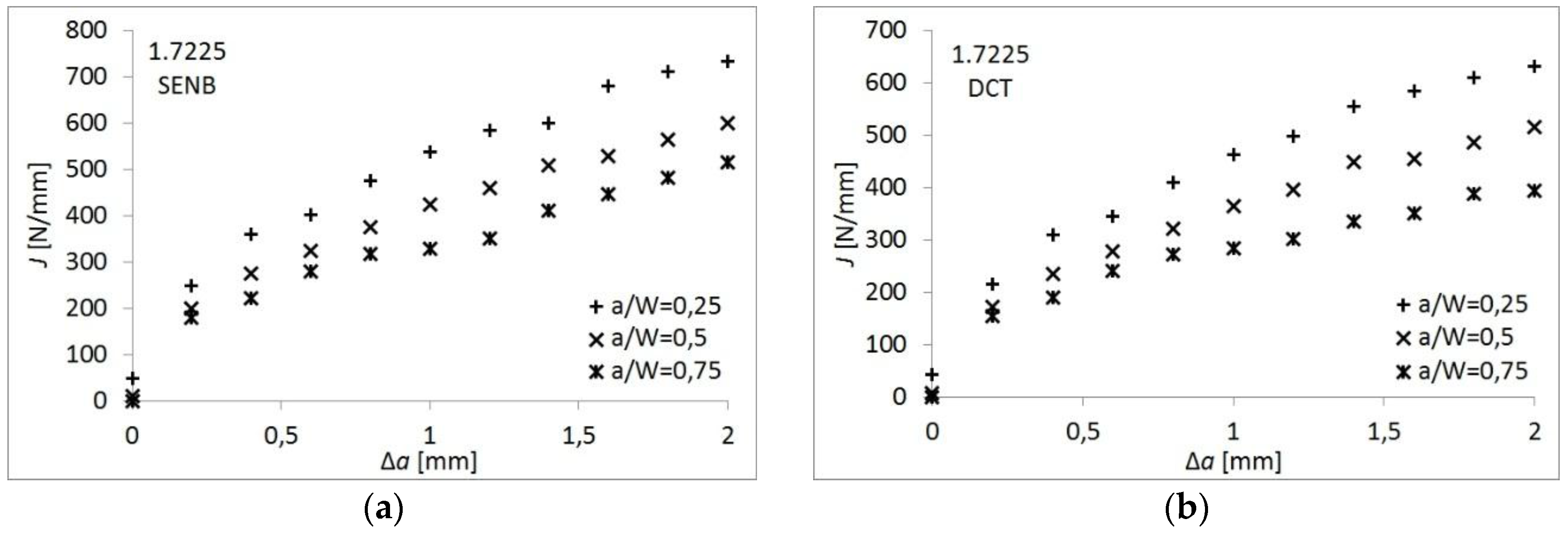
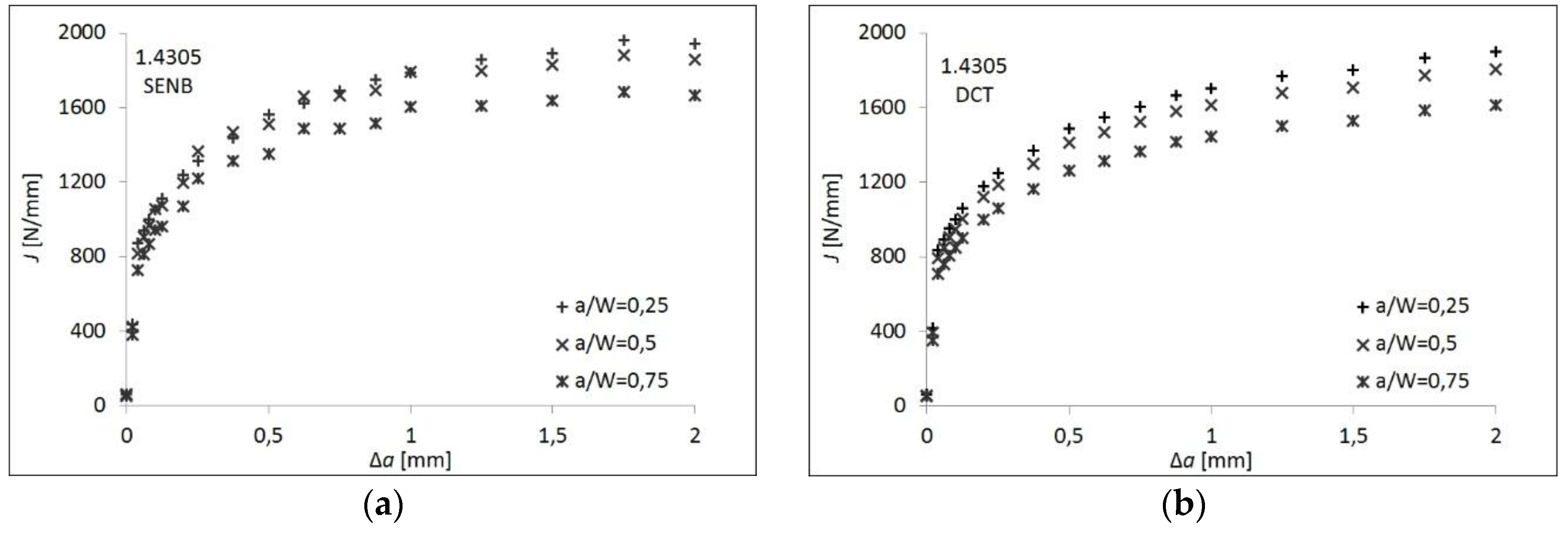
The entire numerical procedure described in Section 2.2 was performed for FE models of SENB and DCT specimens. With respect to the geometry of specimens, initial a/W (crack length/width ratio with W = 50 mm) ratios of 0.25, 0.5 and 0.75 are taken with Δa = 0...2 mm (Δa being crack advance). For every case, J-integral values, as a measure of crack driving force, are calculated and the final results are shown in Figure 7 (for steel 1.4305) and Figure 8 (for steel 1.7225).
4. Discussion
The fracture behaviors of the mentioned materials are given in Figure 7 and Figure 8, using J-integral as a measure of crack driving force. It can be noted that steel 1.7225 has higher resulting values of J-integral than steel 1.4305, making it more suitable for structures that need less susceptibility to fracture. The predicted difference in resistance to crack extension between steel 1.4305 and steel 1.7225 can be related to the different material properties and compositions (Table 1 and Table 2) of the two materials. Steel 1.4305 has a significantly higher value of nickel, which can contribute to the noted behavior. Nickel is usually added at over 8% (here 7.95%) content to chromium-nickel stainless steels in order to increase strength, impact strength, and toughness. It also improves resistance to oxidization and corrosion along with chromium. Chromium is added at over 12% content in stainless steels to significantly improve corrosion resistance. Added benefits are also hardenability, strength, response to heat treatment, and wear resistance.
In numerical modeling, crack geometry (a/W ratios) was kept the same for both materials in relative specimens, so the geometry probably could not contribute to a difference in J values for the two steels.
J-integral values differ for a/W = 0.75 when compared with a/W = 0.25 and 0.5, which are quite similar in terms of values for steel 1.4305. Additionally, higher a/W ratios correspond to lower J-integral values of materials and vice versa. J-integral values obtained using a DCT specimen FE model give somewhat conservative results when compared with ones obtained using the SENB specimen FE model. Experimentally-obtained KIc values and numerically predicted J values cannot be easily compared because J values go beyond the elastic behaviour of the material, where K is appropriate parameter. Further, J is taken as a measure of crack driving force here. Although the mentioned numerical procedure does not give results that can be directly related to ones obtained experimentally, given results can be useful for the assessment of fracture toughness.
The numerically-obtained data, along with experimentally-obtained yield strength, tensile strength, and CVN energy for steels 1.4305 and 1.7225 presented in this paper may be of importance for designers of engineering structures when concerning material selection. In addition, numerical assessment of J-integral could be useful as a predictor of the possible fracture behaviour of a material. Altogether, experimentally- and numerically-obtained data can be used in the design process to assess the possible load capacity of a structure.
Acknowledgments
This work has been financially supported by the Croatian Science Foundation under the project 6876, and by the University of Rijeka under the projects 13.09.1.1.01 and 13.07.2.2.04. Funds for covering the costs to publish in open access publications have been provided.
Author Contributions
Goran Vukelic and Josip Brnic conceived the idea of the research; Josip Brnic performed the experiments; Goran Vukelic analyzed the data; Goran Vukelic performed numerical analysis; Goran Vukelic and Josip Brnic wrote the paper.
Conflicts of Interest
The authors declare no conflicts of interest. The founding sponsors had no role in the design of the study; in the collection, analyses, or interpretation of data; in the writing of the manuscript; or in the decision to publish the results.
Abbreviations
The following abbreviations are used in this manuscript:
| FE | Finite Element |
| DCT | Disc Compact Tension |
| SENB | Single Edge Notched Bend |
| CVN | Charpy V-notch |
References
- Fonte, M.; de Freitas, M. Marine main engine crankshaft failure analysis: A case study. Eng. Fail. Anal. 2009, 16, 1940–1947. [Google Scholar] [CrossRef]
- Zangeneh, Sh.; Ketabchi, M.; Kalaki, A. Fracture failure analysis of AISI 304L stainless steel shaft. Eng. Fail. Anal. 2014, 36, 155–165. [Google Scholar] [CrossRef]
- Moolwan, C.; Netpu, S. Failure analysis of a two high gearbox shaft. Procedia Soc. Behav. Sci. 2013, 88, 154–163. [Google Scholar] [CrossRef]
- Das, S.; Mukhopadhyay, G.; Bhattacharyya, S. Failure analysis of axle shaft of a fork lift. Case Stud. Eng. Fail. Anal. 2015, 3, 46–51. [Google Scholar] [CrossRef]
- Kossakowski, P.G. Simulation of ductile fracture of S235JR steel using computational cells with microstructurally-based length scales. J. Theor. Appl. Mech. 2012, 50, 589–607. [Google Scholar]
- Dai, Q.; Zhou, C.; Peng, J.; He, X. Experiment, finite element analysis and EPRI solution for J-integral of commercially pure titanium. Rare Metal. Mat. Eng. 2014, 42, 257–263. [Google Scholar]
- Huang, Y.; Zhou, W. J-CTOD relationship for clamped SE(T) specimens based on three-dimensional finite element analyses. Eng. Fract. Mech. 2014, 131, 643–655. [Google Scholar] [CrossRef]
- Koshima, T.; Okada, H. Three-dimensional J-integral evaluation for finite strain elastic-plastic solid using the quadratic tetrahedral finite element and automatic meshing methodology. Eng. Fract. Mech. 2015, 135, 34–63. [Google Scholar] [CrossRef]
- Saputra, A.A.; Birk, C.; Song, C. Computation of three-dimensional fracture parameters at interface cracks and notches by the scaled boundary finite element method. Eng. Fract. Mech. 2015, 148, 213–242. [Google Scholar] [CrossRef]
- Zambrano, O.A.; Coronado, J.J.; Rodríguez, S.A. Failure analysis of a bridge crane shaft. Case Stud. Eng. Fail. Anal. 2014, 2, 25–32. [Google Scholar] [CrossRef]
- Fonte, M.; Duarte, P.; Anes, V.; Freitas, M.; Reis, L. On the assessment of fatigue life of marine diesel engine crankshafts. Eng. Fail. Anal. 2015, 56, 51–57. [Google Scholar] [CrossRef]
- Tawancy, H.M.; Al-Hadhrami, L.M. Failure of a rear axle shaft of an automobile due to improper heat treatment. J. Fail. Anal. Prev. 2013, 13, 353–358. [Google Scholar] [CrossRef]
- Bai, S.Z.; Hu, Y.P.; Zhang, H.L.; Zhou, S.W.; Jia, Y.J.; Li, G.X. Failure analysis of commercial vehicle crankshaft: A case study. Appl. Mech. Mater. 2012, 192, 78–82. [Google Scholar] [CrossRef]
- Fuller, R.W.; Ehrgott, J.Q., Jr.; Heard, W.F.; Robert, S.D.; Stinson, R.D.; Solanki, K.; Horstemeyer, M.F. Failure analysis of AISI 304 stainless steel shaft. Eng. Fail. Anal. 2008, 15, 835–846. [Google Scholar] [CrossRef]
- American Society for Testing and Materials (ASTM International). Metals Test Methods and Analytical Procedures; Annual BOOK of ASTM Standards; ASTM International: Baltimore, Maryland, MD, USA, 2005; Volume 03.01. [Google Scholar]
- Brnic, J.; Turkalj, G.; Canadija, M.; Lanc, D.; Krscanski, S. Responses of austenitic stainless steel American iron and steel institute (AISI) 303 (1.4305) subjected to different environmental conditions. J. Test. Eval. 2012, 40, 319–328. [Google Scholar] [CrossRef]
- Brnic, J.; Turkalj, G.; Canadija, M.; Lanc, D.; Brcic, M. Study of the effects of high temperatures on the engineering properties of steel 42CrMo4. High Temp. Mater. Proc. 2015, 34, 27–34. [Google Scholar] [CrossRef]
- Roberts, R.; Newton, C. Interpretive Report on Small Scale Test Correlations with KIc Data; Welding Research Council Bulletin: New York, NY, USA, 1981; pp. 1–16. [Google Scholar]
- Rice, J.R. A path independent integral and the approximate analysis of strain concentration by notches and cracks. J. Appl. Mech. 1968, 35, 379–386. [Google Scholar] [CrossRef]
- Cherepanov, G.P. The propagation of cracks in a continuous medium. J. Appl. Math. Mech. 1967, 31, 503–512. [Google Scholar] [CrossRef]
- Mohammadi, S. Extended finite element method; Blackwell Publishing: Singapore, 2008; pp. 56–58. [Google Scholar]
- Vukelic, G.; Brnic, J. Prediction of fracture behavior of 20MnCr5 and S275JR steel based on numerical crack driving force assessment. J. Mater. Civ. Eng. 2015, 27, 14132–14132(6). [Google Scholar] [CrossRef]
- Narasaiah, N.; Tarafder, S.; Sivaprasad, S. Effect of crack depth on fracture toughness of 20MnMoNi55 pressure vessel steel. Mater. Sci. Eng. A 2010, 527, 2408–2411. [Google Scholar] [CrossRef]
Figure 1.
(a) Test specimen (dimension in mm); (b) testing machine.
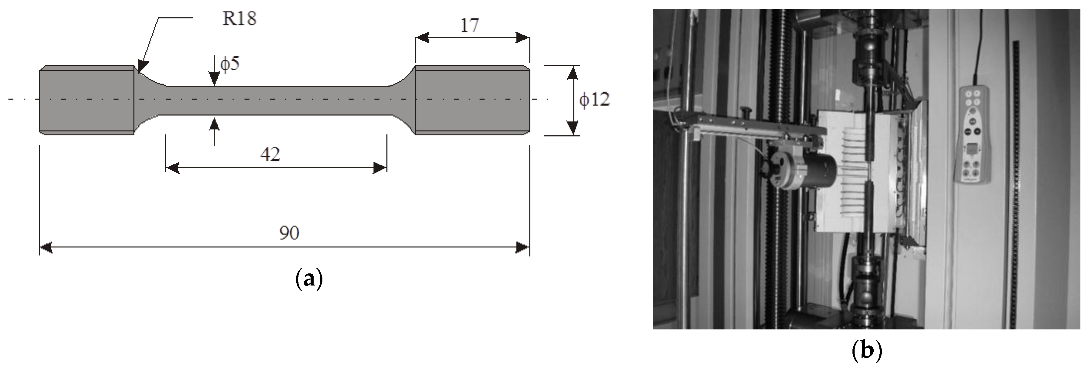

Figure 3.
Optical micrograph of steel 1.4305; as-received material, soft annealed and cold drawn, cross-section of the specimen, aqua regia, 1000×.
Figure 3.
Optical micrograph of steel 1.4305; as-received material, soft annealed and cold drawn, cross-section of the specimen, aqua regia, 1000×.

Figure 4.
Optical micrograph of steel 1.7225; as-received material, soft annealed, cross-section of the specimen, 4% nital, 1000×.
Figure 4.
Optical micrograph of steel 1.7225; as-received material, soft annealed, cross-section of the specimen, 4% nital, 1000×.

Figure 5.
FE model of: (a) SENB specimen; (b) DCT specimen.

Figure 6.
Comparison of numerically-predicted and experimentally-obtained J values for SENB specimens of 1.6310 steel.
Figure 6.
Comparison of numerically-predicted and experimentally-obtained J values for SENB specimens of 1.6310 steel.

Figure 7.
Numerically-predicted J values for steel 1.4305 using FE models of: (a) SENB specimen; (b) DCT specimen.
Figure 7.
Numerically-predicted J values for steel 1.4305 using FE models of: (a) SENB specimen; (b) DCT specimen.

Figure 8.
Numerically-predicted J values for steel 1.7225 using FE models of: (a) SENB specimen; (b) DCT specimen.
Figure 8.
Numerically-predicted J values for steel 1.7225 using FE models of: (a) SENB specimen; (b) DCT specimen.

| Material | C | Cr | Mn | Si | Mo | S | P |
|---|---|---|---|---|---|---|---|
| 1.4305 | 0.047 | 17.4 | 2.0 | 0.584 | − | 0.252 | 0.0323 |
| 1.7225 | 0.45 | 1.06 | 0.74 | 0.32 | 0.17 | 0.018 | 0.014 |
| Material | Ni | Al | V | Nb | W | Cu | Rest |
| 1.4305 | 7.95 | − | − | − | − | − | 71.734 |
| 1.7225 | 0.04 | 0.02 | 0.01 | 0.02 | 0.02 | 0.04 | 97.078 |
© 2016 by the authors; licensee MDPI, Basel, Switzerland. This article is an open access article distributed under the terms and conditions of the Creative Commons by Attribution (CC-BY) license (http://creativecommons.org/licenses/by/4.0/).
Share and Cite
MDPI and ACS Style
Vukelic, G.; Brnic, J. Predicted Fracture Behavior of Shaft Steels with Improved Corrosion Resistance. Metals 2016, 6, 40. https://doi.org/10.3390/met6020040
AMA Style
Vukelic G, Brnic J. Predicted Fracture Behavior of Shaft Steels with Improved Corrosion Resistance. Metals. 2016; 6(2):40. https://doi.org/10.3390/met6020040
Chicago/Turabian StyleVukelic, Goran, and Josip Brnic. 2016. "Predicted Fracture Behavior of Shaft Steels with Improved Corrosion Resistance" Metals 6, no. 2: 40. https://doi.org/10.3390/met6020040
Note that from the first issue of 2016, this journal uses article numbers instead of page numbers. See further details here.