3.1. Optimization of the Process Parameters via the Taguchi Method
In this study, a Taguchi orthogonal array, which can handle five levels of the parameters with three columns and 25 rows, was used. The parameter optimization procedure was done in order to get a welded joint that has the maximum TL by minimizing the HI. HI plays a crucial role in the quality of the joint and indirectly the operation cost. The weld joint quality can be defined as weld bead geometry, mechanical properties and distortions [
25]. Weld bead geometry, which means the bead width and penetration depth, is an important physical characteristic of a weldment, especially for dissimilar laser welding processes [
19]. The appropriate weld bead geometry depends on the HI rate [
22]. A shallower and inadequate penetration depth is related to an insufficient HI rate. Thence, the TL of the welded joint will decrease. However, a higher HI gives a slower cooling rate, and so, in the HAZ, large grain sizes can have poor toughness and decrease in TL. Hence, HI and, consequently, weld bead geometry affect the tensile strength of the joints [
16,
18]. Therefore, in this study, TL and HI were evaluated together as a response variable. Due to the tensile strength being the most important quality indicator of the welded joint, the effect ratio of the TL was determined to be higher, 60%. In determining the effect ratio of the HI, operational cost and weld bead geometry were considered. Namely, this ratio should not be too low because of the insufficient penetration, and also, it should not be too high in terms of cost and decreased strength of the joint. Therefore, it was determined to be 40%. In determining these effect ratios, they have also benefited from operational experience.
The TL of the laser welded joints was experimentally determined using tensile tests. At least three different specimens’ tensile test results’ average were taken. Additionally, HI was calculated by the laser power divided by the welding speed. Due to the scale of the values of TL and HI being different, a normalization process was applied to these values. Equation (3) was used for the normalization of the TL values.
where
Xn is the normalized value,
Xi is the value of the relevant row and
Xmax is the maximum value. Since the objective function was a combination of the TL and HI, it is necessary to express it in the same form. Therefore, before applying Equation (3), the reciprocals of the HI values were taken using Equation (4) to convert the values to the larger the better form.
where
Xp is a pre-normalized value, which was used in Equation (1), and
Xi is the HI value of the relevant row.
The experimental layout for the process parameters, average TL, standard deviations (SD), HI values and normalized values are shown in
Table 3. The
S/
N ratios for the response were calculated. The response column represents the sum of 60% normalized TL and 40% normalized HI. The
S/
N ratios of the process parameters were calculated by using Equation (2), and the effect of each parameter level was determined. As can be seen in
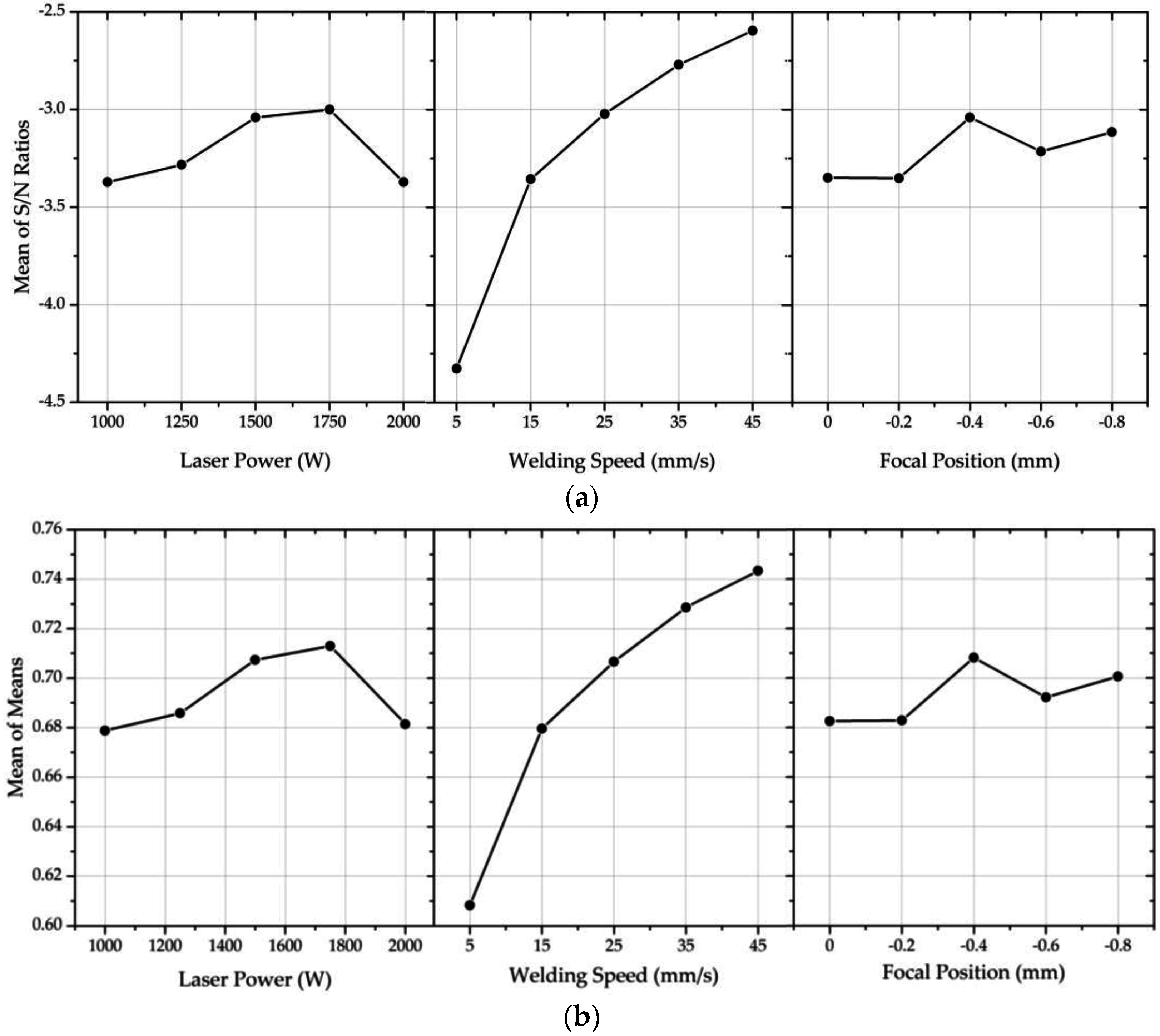
Table 4, welding speed was the most important parameter for the response. Laser power and focal position followed this parameter, respectively.
The
S/
N ratios’ main effect plot showed how each process parameter affects the response characteristic. The means of the
S/
N ratios exhibit a good correlation with the main effects of the mean of means (
Figure 2). This result indicates that process parameters show higher mean values resulting in higher variability. The response seems to be mainly affected by the process parameters, as shown in
Figure 2. It can be seen that the welding speed was the most important process parameter that affected the response. There was a small difference between laser power and focal position; while the focal position plots showed the lowest effect on the response to those parameters.
In this study, the optimal parameter combination was found to be 1750 W for laser power, 45 mm/s for welding speed and −0.4 mm for the focal position. This parameter combination was Sample 20 in the orthogonal array in
Table 3; thus, no additional confirmation experiments were required.
3.4. Microstructure and Microhardness Evolution
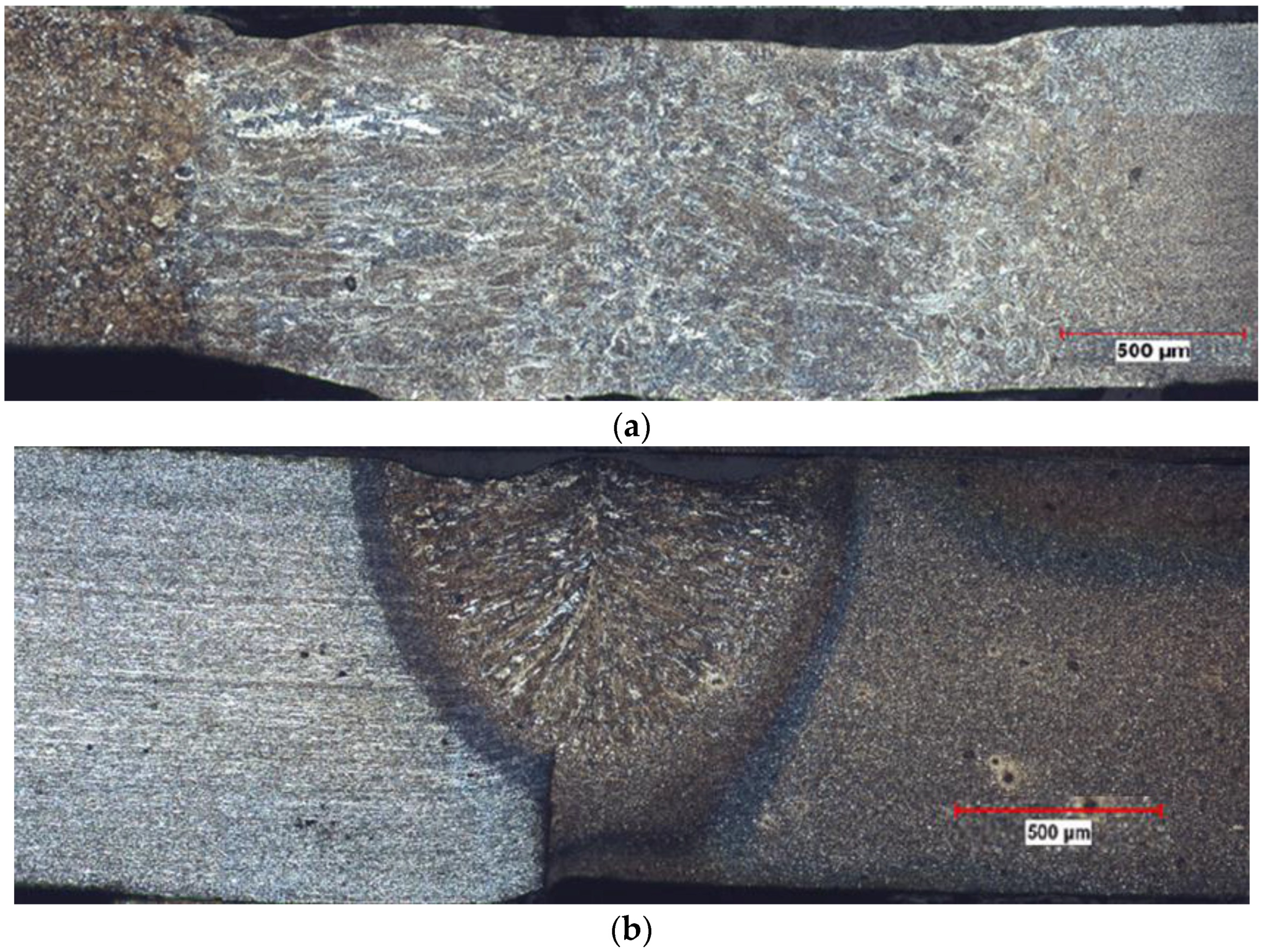
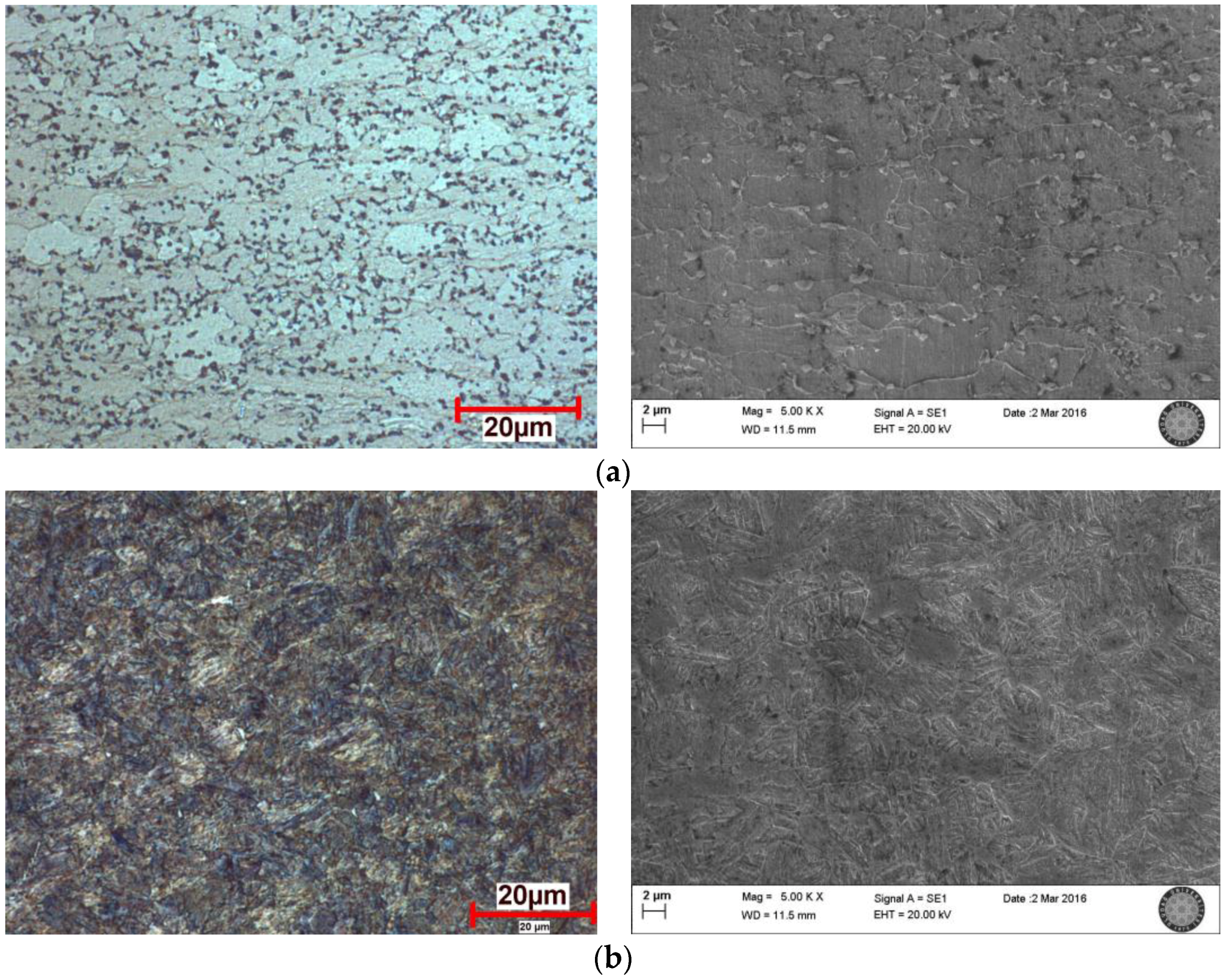
The microstructural examination and microhardness evolution of the selected welds that have the highest (Sample 20) and lowest (Sample 21) response values were discussed. Three different zones, including FZ, HAZ and base metal (BM), were revealed by examining the selected sample’s cross-sections. The BM of the HSLA consisted of a ferrite matrix with carbides dispersed in the grains and at the grain boundaries (
Figure 4a). As shown in
Figure 4b, MART steels were comprised of martensitic microstructures and a small proportion of ferritic and bainitic grains.
In the welding process, final microstructures are affected by peak temperature and the cooling rate of the relevant zones, and carbon equivalent (CE) value resulted from the chemistry of the steels [
29,
30,
31,
32]. Although there are numerous formulae for calculating CE, Yurioka’s formula was used in this study because of its suitability for C-Mn steels [
33]. The CE values of steels were calculated using Yurioka’s formula given by Equation (5) and shown in
Table 6 [
34,
35]. The Ti element was considered as the Nb element because of their similar effect on the steels’ hardenability.
where
f(
C) is the accommodation factor and is calculated as;
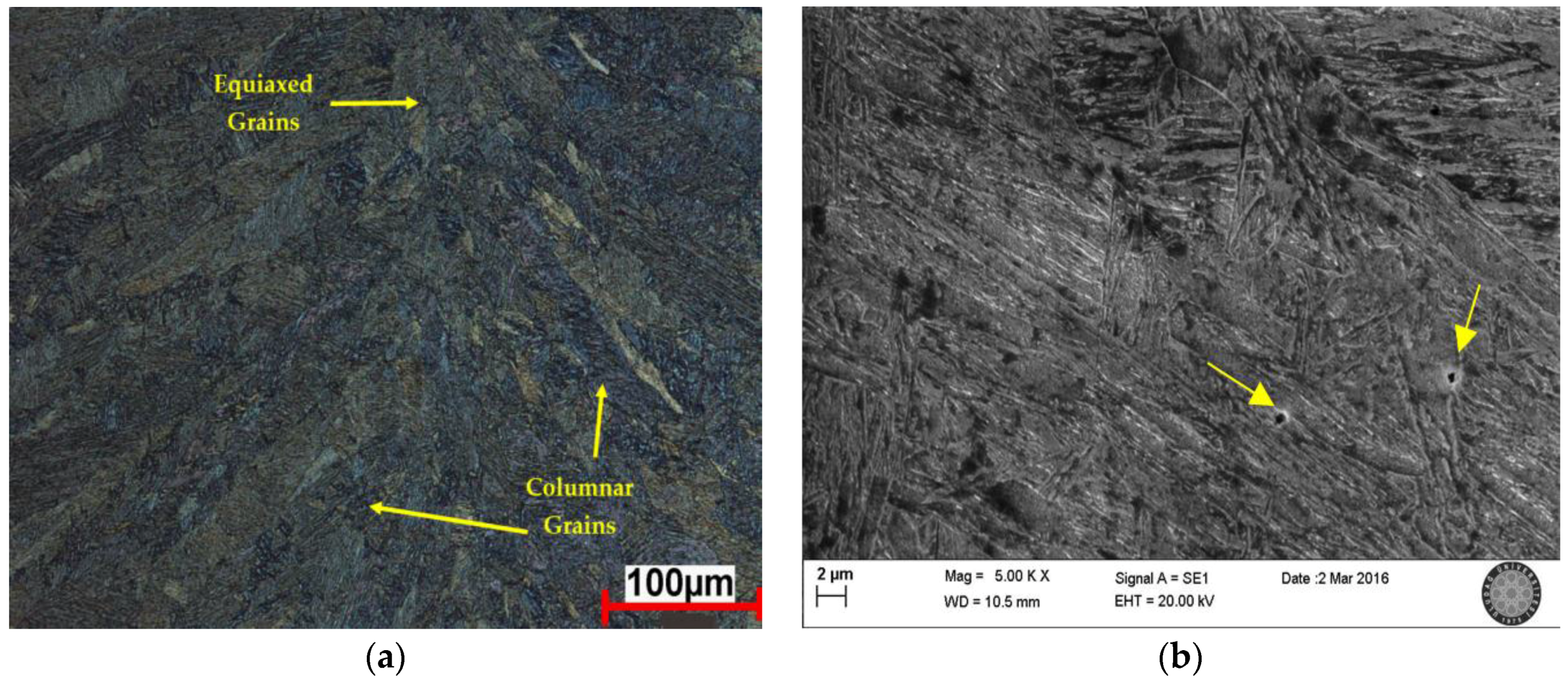
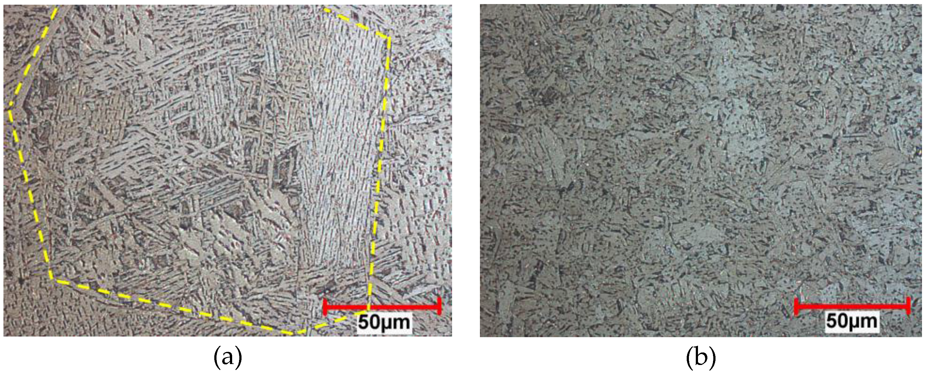
The microstructure of the FZ of Sample 20, with a 0.391 CE value (average of MART and HSLA steels), is predominantly martensite with a bainitic structure (
Figure 5). With the effect of the heat exchange gradient, in the vicinity of the fusion boundary, grains were elongated towards the weld center. However, in the center of the FZ, equiaxed grains were observed (
Figure 5a). Furthermore, due to the lack of shielding gas, as a possible result of the diffusion of some elements, i.e., oxygen and nitrogen from the air, it is thought to be some inclusions in the FZ, which were marked with yellow arrows in
Figure 5b.
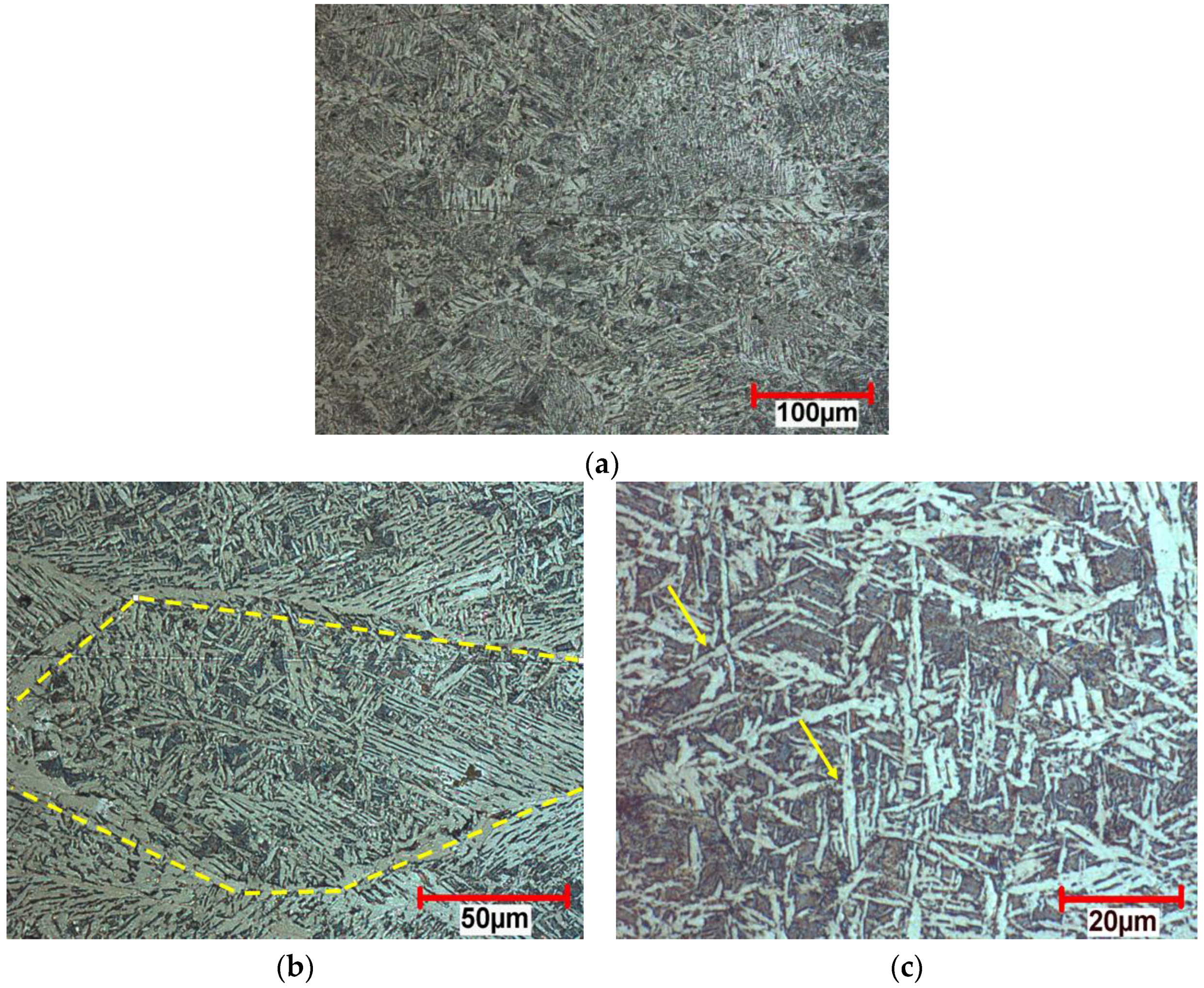
Weld zone microstructures of Sample 21, which have the highest heat input and, of course, slowest cooling rate, are completely different from Sample 20 and not associated with the CE values due to the slow cooling conditions. The FZ of Sample 21 consisted of ferritic microstructures with multiple morphologies, e.g., grain boundary, acicular and Widmanstatten (
Figure 6a). Due to the oriented solidification and slow cooling rate, elongated and extremely coarse grains were revealed. In
Figure 6b, grain boundaries were dashed with yellow, which contain different ferritic structures. Acicular ferritic microstructures can also be seen in
Figure 6. The yellow arrows show the inclusions where acicular ferrites nucleated (
Figure 6c).
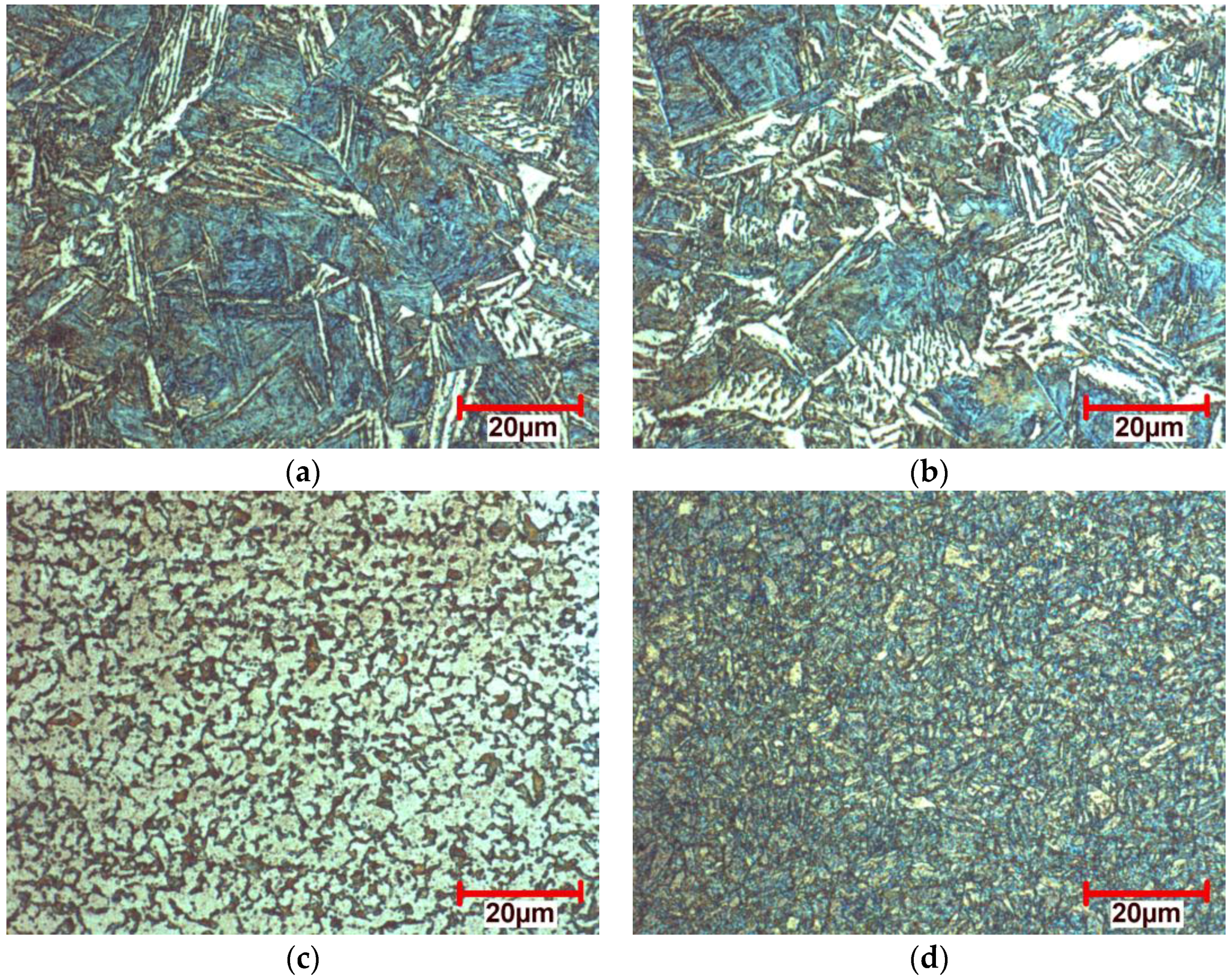
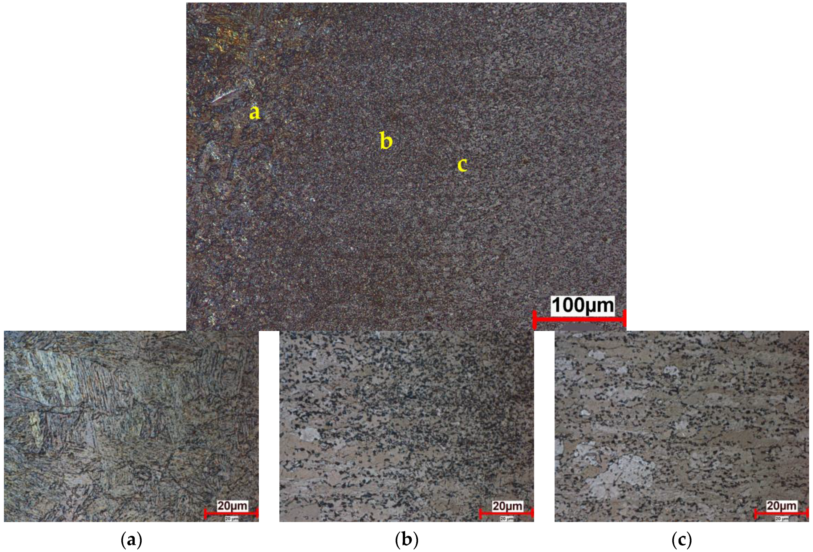
The HAZ of Sample 20 can be divided into five subzones, namely partially molten zone (PMZ), coarse-grained HAZ (CGHAZ), fine-grained (FGHAZ), inter-critical HAZ (ICHAZ) and sub-critical HAZ (SCHAZ). Optical micrographs of these different subzones can be seen in
Figure 7 and
Figure 8. In the microstructural examinations, PMZ could not be observed. Both MART and HSLA steel, in CGHAZ, consisted of martensitic-bainitic microstructure as a result of the transformation of coarsened austenite grains (
Figure 7a and
Figure 8a). While the CGHAZ of MART steel shows a higher proportion of martensitic and lower proportion of bainitic microstructures, HSLA steel shows a higher proportion of bainitic and lower proportion of martensitic microstructures. This can be attributed to the CE values of the steels. A higher CE value promoted the formation of martensite, whereas a lower CE value promoted bainitic structures. Although the FGHAZ of MART steel’s microstructure is similar to CGHAZ, but consisted of finer grains, this zone could not be observed in HSLA steel. In the ICHAZ, where the peak temperature is between A
3 and A
1, the partial transformation of ferrite to a mixture of ferrite and austenite resulted in martensite islands between the fine-grained ferrite matrix and carbides in HSLA steel (
Figure 7b) [
2].
Figure 7b shows a transition zone towards SCHAZ.
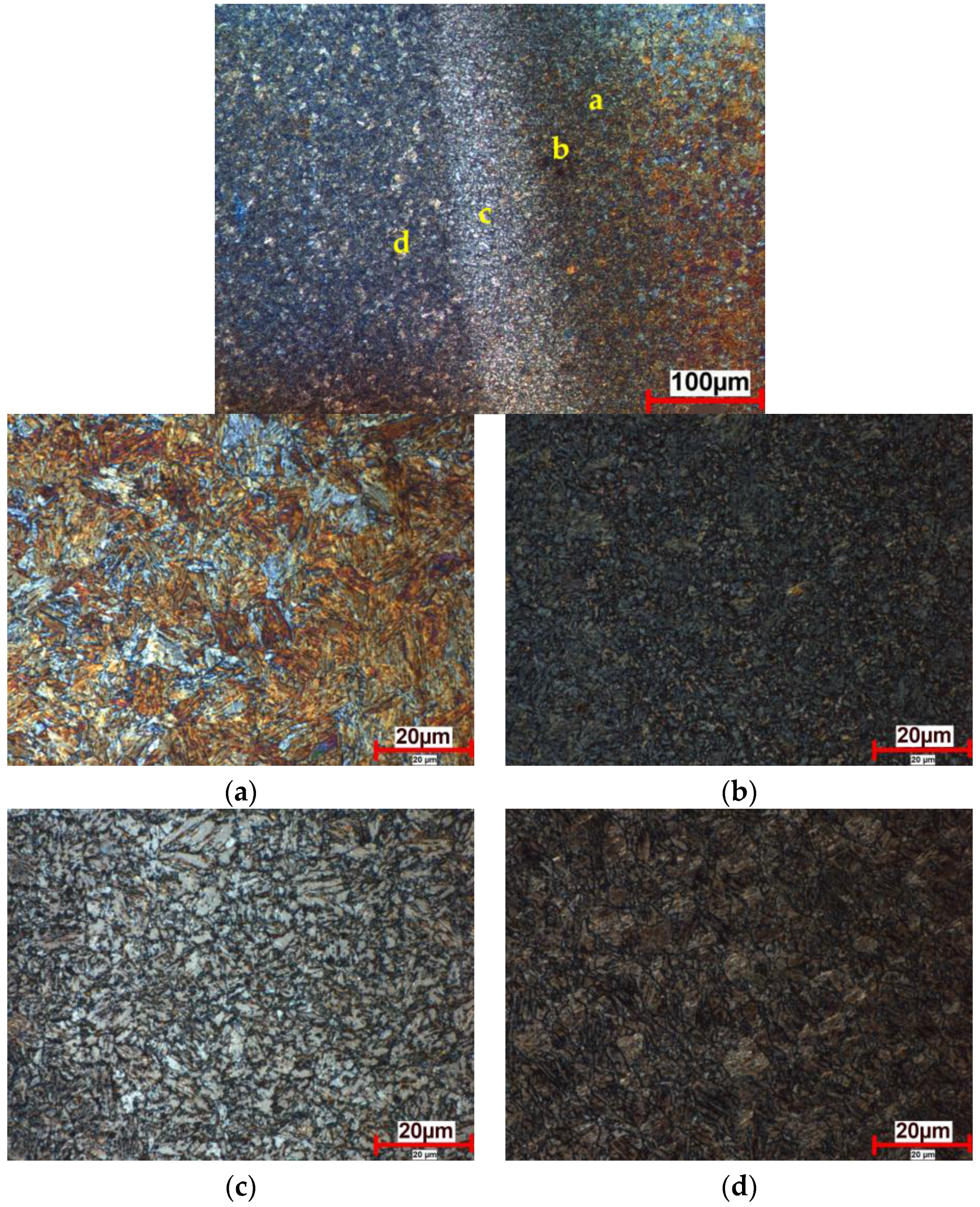
The ICHAZ of MART steel exhibited a dual phase microstructure containing ferrite with fine and well-dispersed martensite. In addition, some portion of the acicular ferritic microstructures can be seen in
Figure 8c. Since shielding gas was not used, nitrogen and oxygen absorption could promote titanium base nitrides, carbo-nitrides and oxide inclusions where acicular ferrites can nucleate [
2,
36,
37,
38]. Furthermore, the slow cooling rate of this zone could induce ferritic structures to be formed.
Figure 8d shows the SCHAZ of MART steel. In this zone, tempered martensite and bainite formed due to the lower peak temperature than A
1. However, it is expected that the coarsening of the carbides occurs in the HSLA side, and there is no difference identified metallographically. This can be related to the thermal stability of the HSLA, which is greater than MART and, therefore, does not have a microstructure that is distinct from its BM [
2].
For Sample 21, the whole weld zone was roughly 11 mm, so only the micrographs of specific zones are presented here. The CGHAZ of HSLA side of Sample 21 consisted of ferritic and bainitic structures and it is shown with dashed lines. The FGHAZ of the HSLA side contains similar, but finer grains with respect to CGHAZ (
Figure 9b). Beside the FGHAZ, coarsening of the carbides occurred in the HSLA side.
In the CGHAZ and FGHAZ of the MART side of Sample 21, as a result of the higher CE, coarse baiting, ferritic and martensitic microstructures were identified (
Figure 10a,b). The ICHAZ, in accordance with the Fe-Fe
3C equilibrium diagram, consisted of fine ferritic structures with small portions of pearlitic structures (
Figure 10c). As expected, under the influence of a relatively high temperature, which is in the range of martensite tempering temperatures, tempered martensite formed in SCHAZ of the MART side (
Figure 10d).
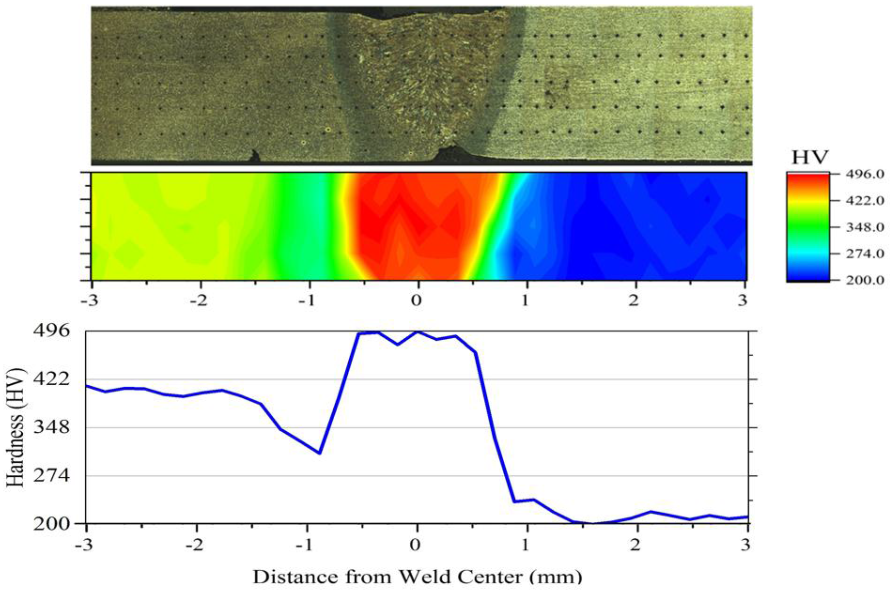
Microhardness measurements were conducted in the various zones of Samples 20 and 21. The microhardness of the BM of the HSLA and MART steels was measured as 213 and 404 Vickers, respectively. The hardness profile of the welded joint section varies significantly because of the phase transformations during the thermal cycle of the welding process.
Figure 11 shows the microhardness map of Sample 20.
Figure 11 also presents the microhardness profile across the mid-section of the sample. Due to the rapid cooling of FZ, each material showed an increase in hardness of FZ relative to BM. The average microhardness value in the FZ is 480 Vickers and varies across the section. This fluctuation is attributed to the mixed microstructure of the FZ. Different hardness of the martensitic and bainitic microstructures could cause the fluctuation of the hardness profile. In addition, various morphologies (i.e., columnar and equiaxed) in FZ could be a reason for the various hardness. However, some researchers have focused to determine an empirical formula for FZ hardness using CE values; in the present study, the measured hardness of FZ is higher than the calculated values using the mentioned formulas [
31,
36]. The calculated hardness values using the formulas given in the literature are 434 HV and 365 HV. In all compared zones, MART steel exhibited higher hardness values due to the higher CE value, which has a significant influence on the hardenability. While the hardness of the HSLA side exhibits a sharp increase through the HAZ up to the FZ, the MART side shows a softening zone in HAZ. The continuous increase trend in the HSLA side was due to the ferritic microstructure of HSLA steel. The tempering zone and ferritic/martensitic dual phase structures in MART steel caused a decrease in hardness.
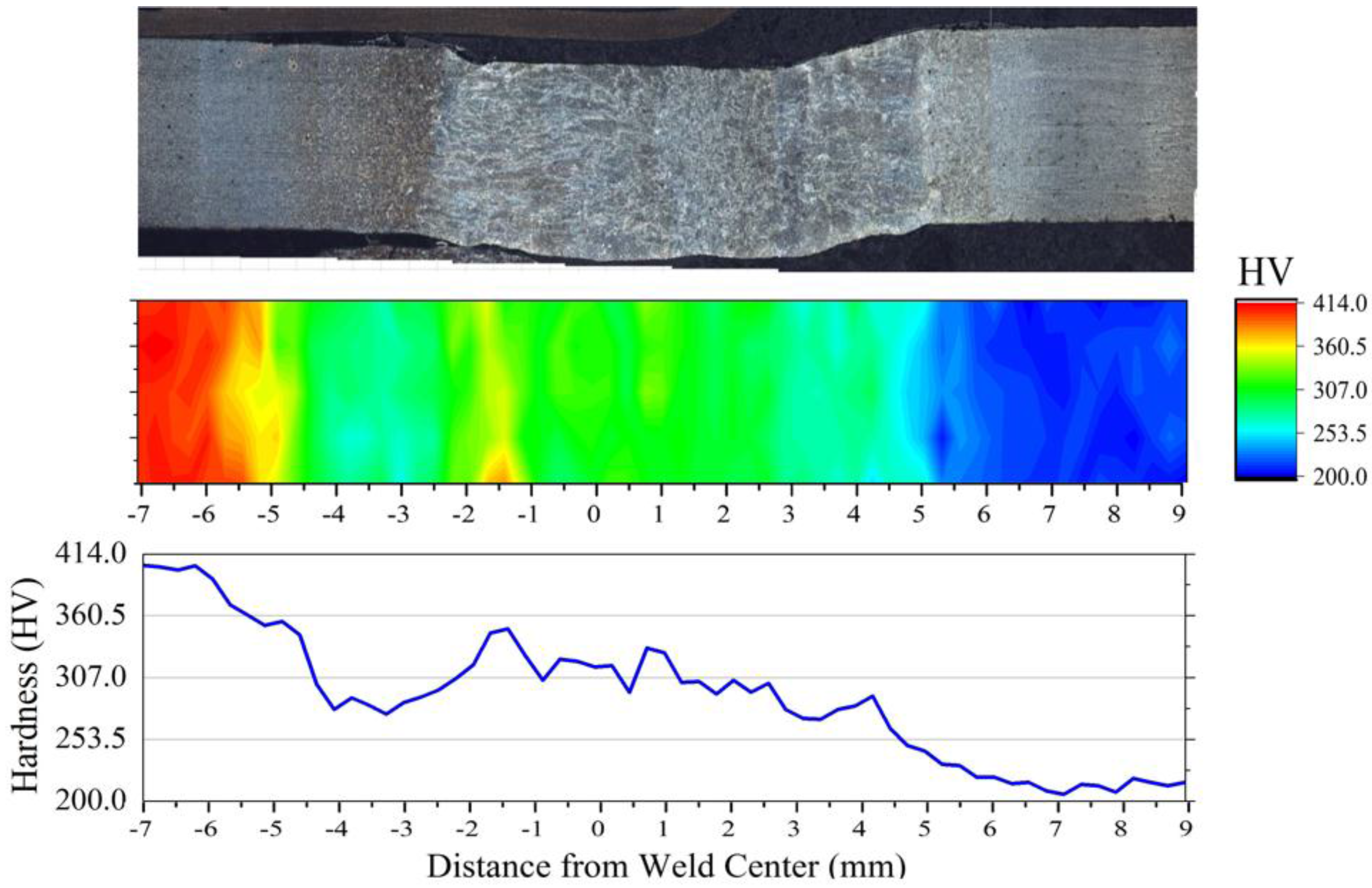
The microhardness map and profile of Sample 21 can be seen in
Figure 12. The highest and the lowest microhardness values were measured in the BM of MART and HSLA, respectively. The highest value is related to the predominantly martensitic microstructure of the BM of MART steel. Among the weld zone of the MART steel, the ICHAZ showed the lowest microhardness corresponding with the ferritic-pearlitic microstructure. The measured microhardness values through the FZ showed a fluctuation, which can be a result of multiple morphologies of ferritic structures. In the HSLA side, microhardness values showed a decreasing trend up to the BM.


