
Development and Numerical Testing of a Model of Equiaxed Alloy Solidification Using a Phase Field Formulation


School of Mechanical and Materials Engineering, University College Dublin, Belfield, D04 V1W8 Dublin, Ireland
*
Author to whom correspondence should be addressed.
Metals 2023, 13(12), 1916; https://doi.org/10.3390/met13121916
Submission received: 6 October 2023
/
Revised: 6 November 2023
/
Accepted: 19 November 2023
/
Published: 21 November 2023
(This article belongs to the Special Issue Modeling of Alloy Solidification)
Abstract
:A computational framework is developed to understand the transient behavior of isothermal and non-isothermal transformation between liquid and solid phases in a binary alloy using a phase-field method. The non-isothermal condition was achieved by applying a thermal gradient along the computational domain. The bulk solid and liquid phases were treated as regular solutions, along with introducing an order parameter (phase field) as a function of space and time to describe the interfacial region between the two phases. An antitrapping flux term was integrated into the present phase-field model to mitigate the amount of solute trapping, which is characterized by the non-equilibrium partitioning of the solute. The governing equations for the phase field and the solute composition were solved by the cell-centered finite volume method using the open-source computational tool OpenFOAM. Simulations were carried out for the evolution of equiaxed dendrites inside an undercooled melt of a binary alloy, considering the effect of various computational parameters such as interface thickness, strength of crystal anisotropy, stochastic noise amplitude, and initial orientation. The simulated results show that the solidification morphology is sensitive to the magnitude of anisotropy as well as the amplitude of noise. A strong influence of interface thickness on the growth morphology and solute redistribution during solidification was observed. Incorporating antitrapping flux resulted in the solute partitioning close to the equilibrium value. Simulations show that the grain shape is unaffected by changes to crystallographic orientation with respect to the Cartesian computational grid. Thermal gradients exerted discernible effects on the solute distribution and the dendritic growth pattern. Starting with multiple nucleation events the model predicted realistic polycrystalline solidification and as-solidified microstructure.
1. Introduction
The mechanical properties of many materials are intrinsically linked to their microstructural evolution. In the realm of metal and alloy solidification, the appearance of complex microstructures is a significant phenomenon. Dendrites, characterized by their multi-branched, tree-like configurations, stand out as a common microstructure pattern. Such formations are frequently seen during metal solidification and the crystallization of supersaturated solutions [1,2]. In solidification, comprehension and control of the size and shape of dendrites has emerged as a key area of interest amongst the scientific community. Nevertheless, practical limitations exist in directly observing the solidification process through experimental means, although much has been achieved in recent years using in-situ X-radiation [3]. Numerical simulations present a valuable alternative as they allow for a visual representation in silico of the phase transition process and help to gain a deeper insight into the microstructure, which is closely associated with mechanical properties. In recent decades, many numerical models have been developed to simulate the evolution of dendritic morphologies during solidification. These include techniques such as level set [4], Monte Carlo [5], cellular automata [6,7,8,9,10,11], and the phase-field method (PFM) [12,13,14]. Amongst the various computational methods, phase-field methods have gained tremendous attention among researchers. In comparison to other simulation methods, the noteworthy advantage of the phase-field method is that the governing equations are expressed in a unified manner throughout the entire computational space, which obviates the necessity of interface tracking [15]. The phase-field method has gained widespread usage in the modeling of complex microstructure changes in a wide range of applications such as solidification, solid-state phase transformation, crystal growth, recrystallization, martensitic transformation, dislocation dynamics, and crack propagation [16,17].
Several phase-field models have been developed for the solidification of pure materials [18,19,20,21,22,23]. The first 2-D PFM for the isothermal dendritic growth of an alloy into highly supersaturated liquid was proposed by Wheeler et al. [24]. They assumed an ideal solution alloy based on a single gradient energy term, , in the phase-field variable, and equal diffusivities in both solid and liquid phases, to simulate dendritic growth based on the minimization of the free energy function; this approach became widely known as the WBM-1 model. In their model, the term was incorporated in the governing equation, but solute trapping was not observed because of neglecting the gradient of solute composition term, . Warren and Boettinger [25] used an isothermal phase-field model to predict the dendritic growth and micro segregation pattern in a binary alloy using entropy formulation.
In a subsequent study, Wheeler et al. developed a new PFM model (WBM-2) [26], which embodied both gradient terms, i.e., and . They recovered the velocity-dependent partition coefficient k(v) through the inclusion in the free energy functional of a term at large velocities using Aziz and Kaplan’s continuous growth model CGM [27]. However, it was confirmed later by others that including the term is not necessary to predict solute trapping. Kim et al. [28] developed another PF model for a binary alloy equivalent to the WBM model, however, with a different definition of free energy density at the interfacial region. Conti [29] discussed the thermal effects on the solidification of binary alloys, and Loginova et al. [30] simulated dendritic morphology and temperature distribution in Ni-Cu binary alloy solidification using phase-field methods. Ohno and Matsuura [31] extended the PFM to a ternary alloy for non-isothermal solidification, and the simulation convergence was investigated. Karma [32] proposed a phase-field method tailored for simulating microstructural evolution in alloys. By integrating an anti-solutal trapping current into the model, he illustrated that it is possible to replicate the dendritic tip velocity and solute distribution of a thin interface, even when using a substantially thicker interface. Lan and Shih [33] incorporated the antitrapping current into the solute diffusion equation and executed an efficient adaptive phase-field simulation, examining non-isothermal free dendritic growth in a binary system subjected to forced liquid flow.
Polycrystalline solidification is a complex process whereby multiple crystals grow simultaneously and interact with each other within a solidifying alloy. This interaction leads to the development of distinctive grain structures, which can significantly influence the material’s mechanical properties. Understanding and modeling this phenomenon is essential for predicting and optimizing the microstructural characteristics of industrially important metals and alloys. Polycrystalline microstructures can be broadly classified in two different types: (i) equiaxed multigrain structures which are formed by the nucleation, growth, and impingement of many crystals, and (ii) polycrystalline growth forms such as dizzy dendrites, spherulites, etc., in which new grains nucleate at the solidification front. [34]. Over the years researchers have explored various types of phase-field method to simulate polycrystalline solidification. Jou and Lusk [35] examined the development of foam-like multigrain configurations within a homogeneous, single-component isotropic system by applying a theory based on a scalar order parameter and observed minor deviations in the growth rate and JMAK theory. Elder et al. [36] formulated a model for the multigrain solidification of an isotropic eutectic system, using a structural order parameter, concentration field, and Langevin noise-induced nucleation.
Gránásy et al. [37] employed phase field theory based on a free energy functional from the WBM model to examine the growth of multiple particles in a binary system, yielding results that aligned well with experimental findings by Pradell et al. [38]. Morin et al. [39] simulated anisotropic growth by using a phase-field model with distinct crystallographic orientations for solidification, characterized by a free energy density with multiple wells, disrupting the usual rotational symmetry. Nonetheless, the model falls short of capturing real-world physical situations because it results in the creation of diffuse grain boundaries.
Steinbach et al. [40] introduced a multiphase-field (MPF) model in which each crystal was represented by a different phase-field order parameter, often resulting in the need for thousands of such fields to effectively simulate multi-grain scenarios. Followed by Fan and Chen [41], Tiaden et al. [42], Diepers et al. [43], and Krill and Chen [44] also used MPFs, which offer highly adaptable methodologies for modeling the nucleation and growth of particles with arbitrary crystallographic orientations. However, a significant limitation of these models is the intentional disruption of the free energy’s rotational symmetry to accommodate a specific number of phase fields. Kobayashi et al. [45] pioneered a model for polycrystalline solidification that not only accounted for crystallographic orientation but also preserved the rotational invariance of the free energy by introducing a non-conserved orientation field (r,t), which determines the local orientation angle and thus the inclination of crystal planes within the laboratory reference frame. This technique was later adapted to characterize the competitive growth of anisotropic particles, such as the dendritic solidification observed in undercooled single-component (Kobayashi et al. [9]) and binary liquids (Warren et al. [46]). Granasy et al. modified the expanded orientation field to encompass the liquid phase, varying it across both space and time [47].
In this paper, we employed the Warren and Boettinger [25] formulation and adopted the antitrapping current scheme of Karma [32] to simulate the dendritic growth in a binary Ni-Cu alloy under isothermal conditions. The simulation results were compared with the findings of Lan and Shih [33] at different values of antitrapping flux. Furthermore, we revisited the effect of various computational parameters such as interface thickness, interface energy anisotropy, noise amplitude, and initial orientation on the equiaxed dendrite. We also investigated the effect of an applied thermal gradient on the growth morphology and composition variation at various values of the thermal gradient. Finally, the above phase-field model by Warren and Boettinger [25] was used to simulate a fixed number of crystal particles under an isothermal condition using a new cell capture-based orientation scheme.
The structure of this paper is delineated as follows: Section 2 offers a concise overview of the governing equations and the numerical implementation approach. In Section 3, we present our results and compare them with previous studies. Finally, conclusions derived from our simulations are encapsulated in Section 4.
2. Methodology
This section presents the initial phase-field model for the solidification of a binary alloy based on the Warren and Boettinger model. The governing equation for solute transport was then modified by adding an antitrapping flux term. The temporal evolution of the phase field and the composition field equations were solved using a bespoke computational solver based on the open-source toolbox OpenFOAM. We employed the Warren and Boettinger [25] phase-field model for polycrystalline solidification and utilized a cellular automaton-like cell capturing method to conduct the solidification process with a predetermined number of crystals.
2.1. Governing Equations
This section gives a brief description of the governing equations for the present phase-field model of alloy solidification. In the phase-field model, an auxiliary continuous order parameter or phase-field variable, denoted as (x, y, t), is employed, which indicates the physical state of the system at each point. The order parameter is set to 0 in the solid phase and 1 in liquid phase and varies smoothly between 0 and 1 across a narrow interfacial region. The position of the interface is obtained from the numerical solution for the phase-field variable at positions where ϕ = . The governing equations for the present model are obtained based on the Helmholtz free energy functional defined by Warren and Boettinger [25]. The temporal evolution equation for the phase field and solute field are obtained by the Allen–Cahn equations [48] for the non-conserved order parameter and the Cahn–Hilliard [49] equation for the conserved order parameter C in a similar manner as described in [25]. In the following equations, ∇ is the del differential operator.
Here, C denotes the composition of the solute, , and R indicates the molar volume and gas constant, respectively. is the diffusion coefficient related to the composition and will be defined later. The superscript/subscript A and B denote the two components of the binary alloy A and B.
Here, is the mobility of the phase field which can be expressed as the weighted average value of the mobilities of components A and B; and as = (1C) + C. The terms and are expressed in terms of the system temperature and phase-field variable as
The terms and denote the barrier height for the double-well potential functions, indicate the melting temperatures, and and signify latent heat of fusion per unit volume for the component A (solute) and B (solvent), . The function h is a steep, smooth function which has minima at bulk phases, i.e., where = 0 or 1, with h= 0 and h; denotes the derivative of h. In the present model, h was chosen as h. The choice of this function assures that for a single-phase solid or liquid = 0 or 1 everywhere in the bulk phases, respectively, and the equation reduces to an ordinary solute diffusion equation by the definition of and h. The function is a double-well function that attains its minimum value in the bulk phases, i.e., = 0 and holds the relation 30 , where is the derivative of g. is the diffusion coefficient related to the composition field given by
At ϕ = 0 (solid) = and at ϕ = 1 (liquid) = , where and are the classical diffusion coefficients in the solid and liquid, respectively.
2.1.1. Anisotropy
In many materials, including metals, the surface energy at the solid–liquid interface and the kinetic coefficient are orientation-dependent, leading to anisotropy which significantly influences crystal growth and dendrite morphology [18]. The most common approach to include anisotropy in a phase-field model, particularly in two-dimensional spaces, involves making the gradient energy coefficient , orientation-dependent. This is based on the direction of interface growth, expressed as = , where 1 + δcos j (()).
Here, δ denotes the strength of anisotropy, j represents the mode number (which is 4 for a cubic material and 6 for a hexagonal material), and is the initial orientation with respect to the reference axis. The term denotes the angle between normal to the interface and reference axis, which can be obtained from the gradient of the phase-field parameter with the following relation:
With incorporation of anisotropy, the governing phase field equation can be expressed as
2.1.2. Antitrapping Current
To mitigate the spurious effects of solute trapping, we incorporated an antitrapping current analogous to the approach introduced by Karma [32]. This antitrapping current supplies a solute flux normal to the diffuse interface from the solid into the liquid, thereby counteracting the tendency of the phase-field model to exhibit unphysical levels of solute trapping. The antitrapping term Jat is added to the composition equation as
Here, a indicates the antitrapping constant.
2.1.3. Thermal Fluctuations at the Interface
It was shown previously by Warren and Boettinger [25] that addition of stochastic noise causes fluctuations at the solid–liquid interface, which leads to the development of a dendritic microstructure with more side branches. To simulate realistic dendritic growth or to mimic the effect of imperfections and inhomogeneities at the solid–liquid interface, random perturbations were added to the governing equations in a similar way as proposed in [25] by modifying the phase field equation as
Here, α denotes the noise amplitude, and r is a random number between −1 and 1. The function , as described above, ensures that the disturbance is added only at the solid–liquid interfacial region.
2.2. Estimation of the Phase-Field Parameters
The computational parameters used in the present phase-field model can be estimated using the relation outlined in Table 1 by choosing interfacial thickness as an input parameter.
The parameters and denote the solid–liquid surface energy of a stationary planar interface and indicate the linear kinetic coefficient. The parameters and , where , denote the solid–liquid interface thickness, and and indicate the melting points of the two components A and B, respectively.
2.3. Numerical Simulation
In this study, the governing equations for the phase-field model were implemented in C++ code using the open-source software OpenFOAM (foam-extend-4.0), utilizing its built-in libraries and utilities. The governing equations were discretized using the cell-centered finite volume method with uniform grids. We utilized an implicit Euler scheme to iteratively advance the phase field and composition equations over time. For optimal load distribution and to mitigate the overhead associated with unnecessary parallelization processes, we utilized the standard memory parallelization techniques provided by OpenMP.
3. Results and Discussion
3.1. Initial and Boundary Conditions
We performed the simulations on the 2D computational domain schematically shown in Figure 1. The spatial grid spacing was set to be = = 46 nm with 750 cells (unless specified otherwise). This grid spacing was small enough to resolve the required fields in the interfacial region accurately. The interface thickness was selected as an input parameter, slightly larger than the grid spacing.
The simulations commenced with a solid () circular seed of initial radius r (minimum required to prevent remelting and to ensure successive growth) at the center of the computational domain, as shown in Figure 1. The thermophysical properties of the binary Ni-Cu alloy used in the present simulations were obtained from the Warren and Boettinger paper [25]. The system contains a supercooled Ni-Cu melt with an initial composition = 0.40831, corresponding to an initial supersaturation of 86%, for which the liquidus and solidus temperatures are 1594.5 K and 1570.5 K, respectively. Given crystallographic directions <100> and <010> aligning with the X-axis and Y-axis, respectively, the fourfold symmetry ensures that simulating a quarter of the domain is adequate for the present simulation initiated by a small quarter disk. At the symmetric and far-field boundaries, the no-flux condition was imposed for the composition and phase field.
We discretized the governing equations using a cell-centered finite volume method on structured orthogonal grids. We employed the Euler scheme for temporal discretization. To tackle the gradient computations, we utilized an advanced extended least squares method and the Gauss linear scheme for the divergence terms. We adopted the Gauss linear corrected scheme for the Laplacian or diffusion terms. For the composition field and the phase field, we adopted the Preconditioned Conjugate Gradient (PCG) solver with the Diagonal Incomplete Cholesky (DIC) preconditioner and a tolerance of 1 × for both the fields. The simulations ran with a time step size of 1 × s.
3.2. Isothermal Free Dendrite Growth
For isothermal solidification, the governing equations of the phase field (Equation (7)) and composition (Equation (8)) were solved. We used the same value of initial undercooling as that used in the Warren and Boettinger paper [25], i.e., 20.5 K, resulting in the system temperature T = 1574 K. Figure 2 shows the morphology of the dendrite (2a,2c) and composition field (2b,2d) at t = 1 ms and t = 2.4 ms, respectively, for an equiaxed dendrite growth inside an undercooled melt under isothermal conditions.
The simulated morphology depicts the evolution of primary and secondary dendritic arms. At the early stage of the simulation, the dendrite extends its primary arms aligned with the crystallographic direction. Normal to the primary arm, smaller secondary arms engage in competition; some become overgrown and disappear, while others grow preferentially along the direction perpendicular to the primary arms. The roots of the secondary arms are significantly narrower, and the secondary arms widen as they extend from their roots.
From the composition field shown in Figure 3, it can be observed that the primary arm has a low concentration compared to the region in between the secondary dendritic arms. This phenomenon, known as micro-segregation, arises during solidification. This difference in concentration arises due to solute redistribution during solidification, where the primary arm, forming initially, rejects more solute, leading to a solute-enriched liquid environment. As a result, when the secondary arms form in this solute-abundant environment, they possess a slightly different concentration than the primary arm. The dendrite center exhibits low concentration, which does not vary much along its length (see red curve in Figure 3). The tip velocity of the dendrite is plotted at different times, as shown in Figure 4.
The observed plateau in tip velocity indicates the achievement of a near-steady state, registering a value of 13.95 mm/s. The calculated value of the steady state tip velocity in our present phase-field model closely matches the value of 13.99 mm/s reported by Loginova et al. [30] for their study on isothermal solidification of the same Ni-Cu binary alloy. In general, the simulated morphology and composition profile of the dendrite is in accordance with the result published in [25]. These agreements with previously published work verify our new model, building confidence for its future development.
3.3. Effect of Interface Thickness
Interface thickness (the width over which the phase transition occurs, indicated by W in the present paper) plays a vital role in terms of accuracy and computational efficiency. To understand the effect of interface thickness on our present phase-field model, we performed simulations for different values of interface thickness, which is a factor of the standard value of the interface thickness used in [25]. The simulations were performed using a square computational domain (23 mm × 23 mm) and varying the number of mesh points. The calculated morphologies and solute profiles for different interface thicknesses are shown in Figure 5.
The dendritic structure illustrated in Figure 5 reveals that a reduced interface thickness fosters the growth of more secondary branches, which is not observed with the thickest interface, as it tends to suppress some of the finer dendritic features. Also, from the plot of tip velocity vs. time (Figure 6) it can be seen that for a higher value of interface thickness (73.4 nm) the tip velocity is lower. This may be because a thicker interface spreads the solute concentration gradient over a larger distance which leads to a reduced driving force for growth as the difference in concentration between the dendrite tip and the surrounding melt becomes less pronounced.
The plot of solute composition along the primary dendrite arm is shown in Figure 7. As the interface thickness reduces, the concentration buildup in the liquid, at the tip position, increases, and the concentration profile in the liquid shows a steeper gradient. Contrastingly, the thicker interface results in a more gradual change in concentration.
We calculated the normalized growth driving force = , where and are the tip concentrations of the dendrite obtained from our phase-field model and is the far field concentration. The solute partition coefficient (k) or the chemical segregation was calculated using the definition of Ahmed et al. [33] by the ratio = = . We also calculated the Peclet number using the tip radius and tip speed by the relation . Based on the Peclet number, the driving force based on the classical Ivanstop solution [50], expressed as
The calculated values of different kinetics parameters for the dendrites at different values of interface thickness are shown in Table 2.
In Table 2, the observed data clearly indicates a reduction in the dendrite tip radius as the interface thickness decreases. This behavior can be attributed to a combination of factors inherent in the phase-field model and the physical processes. As the interface thickness is reduced, the transition from liquid to solid becomes more abrupt, leading to a more pronounced curvature at the dendrite tip due to a rapid change in concentration over a shorter distance, as shown in the composition profiles in Figure 7. Additionally, as the interface becomes thinner, the energy barrier between the liquid and solid phases is more localized near the dendrite’s tip, promoting a smaller tip radius as the system tends to minimize the interfacial energy. Similar behavior of variation in the tip radius and interface Peclet number was reported in the literature by Lan and Shih [33] and Warren and Boettinger [25]. Furthermore, from the values tabulated above, it is clear that as the interface thickness reduces, the solute partition coefficient is closer to the equilibrium value. Additionally, as the interface thickness diminishes, there is an increase in the normalized driving force. This can be associated with the composition profile depicted in Figure 7, a convergence pattern similarly observed in previous work by Lan and Shih [33]. In general, it is desirable to keep the interface thickness as small as possible; however, reducing interface thickness significantly increases the computational cost as it requires larger grid points/elements for a particular domain size and a higher value of temporal resolution. Hence, for the subsequent calculation, we will use an interface thickness W = 48.9 nm as used in the original WBM paper [25].
3.4. Effect of Interface Anisotropy
In this section, we investigate the effect of interface energy anisotropy (δ) for equiaxed dendrites by keeping the interface thickness constant. We performed simulations under isothermal conditions for different values of the anisotropy parameter delta ranging from 0 to 0.067.
From Figure 8, it is evident that small δ values (0 to 0.001 in our present simulation) result in growth morphologies that are more rounded or have irregular rosette-like shapes. This phenomenon can be attributed to the dynamics of the phase-field model and the underlying physics of dendritic growth. A dendritic tip’s stability is highly dependent on anisotropy. According to the Mullins–Sekerka instability, when a system is isotropic or the anisotropy is very low, any small perturbation in the growing interface can grow uncontrollably, leading to repeated tip splitting. Since the anisotropy does not energetically favor any specific direction for growth, this results in chaotic branching patterns that can resemble random or chaotic structures. A similar growth morphology was reported by Wheeler et al. [20] and Karma and Rappel [23] in their findings.
As the anisotropy parameter increases, the solid–liquid interfacial energy becomes strongly anisotropic and results in dendrites with well-defined branches and dendrite tips becoming sharper. From the tip velocity of the dendrite for various values of anisotropy, as shown in Figure 9, it can be observed that with the increase in strength of anisotropy, the dendritic growth velocity also shows a corresponding increase. This is because a higher value of anisotropy results in a stronger directional preference for the dendrite arms to grow and the tip can advance more rapidly along the favorable crystallographic direction.
The composition profile along the primary dendritic arm is shown in Figure 10 for various values of the anisotropy parameter. The solute diffusion layer, a region near the solid–liquid interface, forms due to the local solute redistribution and diffusion during solidification, resulting in a concentration gradient of solute atoms. Due to anisotropy, dendrites grow preferentially along certain crystallographic directions, and they reject solute atoms into the surrounding liquid. This leads to a solute buildup in the liquid regions between the dendrite arms, causing solute enrichment in these specific inter-dendritic regions. This anisotropic growth and diffusion of solute results in a complex composition profile, which includes solute-rich regions between the dendrites (interdendritic regions) and solute-poor regions present within the dendrite arm, as shown in Figure 8.
From Figure 10 we see that, as d increases and the dendrite form becomes finer and with more side-branching, solute can be rejected across a much larger solid–liquid interfacial area, and so less is rejected ahead of the primary tip.
3.5. Effect of Antitrapping Parameter
Solute trapping, characterized by decreased solute partitioning or non-equilibrium solidification at the interface, occurs when solute atoms are not uniformly distributed as expected. This results in a gradual decrease in the concentration gradient across the interface as the solidification rate increases [51]. We investigated the effect of an anti-solutal trapping current in our present phase-field model as described in Section 2. Simulations were performed with two different values of antitrapping constant a = 0 and a = 0.707 for an interface thickness W = 48.9 nm. Note that a = 0 indicates the simulation without the antitrapping current, and a = 0.707 indicates turning the antitrapping current term on during the simulation. The solute composition profiles without and with the antitrapping current are shown in Figure 11.
It can be observed from the composition profile that, with the antitrapping current, the growth morphology is similar to that obtained for a lower interface thickness, as shown previously in Figure 5. The solute distribution profile along the direction of the primary dendritic arm for the two different values of antitrapping current is shown in Figure 12.
It is clear that the antitrapping effect is to decrease the composition of the growing solid. By incorporating the antitrapping term, the solute composition at the dendrite tip is significantly higher than without the antitrapping term. Moreover, without the antitrapping current, the solute profile is shifted more towards the melt side, which is due to the larger growth rate of the dendrite. The tip velocity of the dendrite, driving force , tip radius, normalized driving force, and the solute partition coefficient for different values of antitrapping current are given in Table 3. We also compared our calculated values with those of Lan and Shih [33].
The values derived from our current implementation align very closely with those reported by Lan and Shih [33]. From the above simulation results, it can be concluded that with the antitrapping current, the solute partitioning coefficient k is close to the equilibrium partition coefficient. This observation aligns with what was noted when reducing the solid–liquid interface thickness earlier. However, minimizing interface thickness is not practically feasible for extensive simulations involving larger domains due to the substantial increase in computation time. Therefore, integrating the antitrapping current into the phase-field model for diffusion-controlled growth permits simulations at greater interface thicknesses while preserving computational precision.
3.6. Effect of Noise Parameter
Introducing artificial noise can make the simulation more realistic and comparable to experimental observations, which inherently contain some random perturbations. To explore the influence of artificial noise at the solid–liquid interface, we conducted simulations at different amplitude values of noise α under isothermal conditions. Figure 13 shows the snapshots of dendrite morphology in an undercooled melt for Ni-Cu alloy with different perturbation intensities.
As the amplitude of the noise α increases, it induces a local non-equilibrium condition favoring the initiation of new side branches, leading to dendritic structures with a higher number of secondary arms that would not form without noise, as shown in Figure 13. The thermal noise introduces stochastic fluctuations in the phase-field variable and/or composition field, creating local instabilities along the primary dendrite arm, thereby adding a layer of complexity to the dendritic structure. We plotted the solute composition profile (Figure 14a) and tip velocity (Figure 14b) along the primary dendrite arm for various values of noise magnitude α after t = 2 ms.
As illustrated in Figure 14a, the solute composition profile indicates that the noise amplitude exerts negligible influence on solute redistribution and partitioning. The peak composition values remain consistent across various α values. Concurrently, Figure 14b depicts the primary dendrite tip velocities, which stay relatively constant for different values of the noise magnitude parameter. This behavior can be attributed to the fact that the solute redistribution near the interface at the primary tip is unaltered by the noise magnitude, leading to the stability of tip velocity.
3.7. Effect of Initial Orientation
To investigate the accuracy of the implementation of the present phase-field model, simulations were performed for different values of initial orientation for free dendritic growth in an undercooled melt.
Initially, a solid nucleus with a radius r is placed at the center of the computational domain filled with a supersaturated liquid. The values of initial orientation used in the present simulation are 0, π/18, π/6, π/4, and π/3, respectively. The boundaries of the computational domain were assumed to be in a zero flux condition.
As depicted in Figure 15, dendrites grow fast into the melt along the preferred directions corresponding to their given orientation angles, and the primary arms of the dendrites are almost the same length (approximately 13.8 μm) for different values of . The tip growth velocity , measured according to the positions of the isolines ϕ = 0.5 of the dendrites, is plotted as a function of solidification time in Figure 16. It can be observed that the tip velocities at different orientations coincide, which indicates that the growth is independent of the initial orientation, and the results are consistent with the simulation results in Chen et al. [52], providing further verification of our new model.
3.8. Non-Isothermal Dendritic Growth
To understand the effect of thermal gradient on the morphology and composition profile of equiaxed dendritic growth on a Ni-Cu binary alloy, we performed simulations under the effect of a constant temperature gradient across the computational domain. For these simulations, the temperature variation was characterized by Equation (12).
Here, X denotes the length of the computational domain, and G is the thermal gradient. We initiated our simulation by introducing a circular seed with an initial radius of 23 nm, positioned at the center of the computational domain. For the purpose of this study, we subjected this nucleus to varying thermal gradients, specifically within a range of G = K/m to G = K/m. Additionally, for a comparative analysis between non-isothermal and isothermal growth conditions, we conducted a simulation for G = 0, ensuring an isothermal condition prevailed throughout the domain. Throughout the boundaries, no-flux conditions were consistently maintained across all fields. Figure 17 depicts the temperature distribution across the length of the computational domain for different magnitudes of G.
Figure 18 shows the dendrite morphology and solute distribution at t = 0.7 ms, for various values of G. Without a thermal gradient, dendritic growth manifests as four symmetrical primary arms. Conversely, introducing a thermal gradient alters the growth morphology and the solute distribution. This is particularly relevant to additive manufacturing, where solidification occurs in a thermal gradient.
A steep gradient creates a larger driving force pushing the solidification front to move rapidly on the cooler right-hand side, resulting in larger and coarser dendritic structures. The dendrite adopts a predominantly conical shape rather than a symmetrical dendritic form. Analyzing the compositional profile along the primary dendritic arm under various thermal gradients, as illustrated in Figure 19, it becomes evident that the equilibrium redistribution concentration during non-isothermal solidification, on the cooler side, is reduced compared to its isothermal counterpart.
In the absence of a temperature gradient, the solute segregation is symmetrical. This leads to a composition gradient along the primary dendrite axis: solute-lean at the core and solute-rich at the front. On the contrary, when subjected to a thermal gradient, the concentration profile does not show symmetrical distribution. This asymmetry arises due to the difference in the growth rate of the two primary arms (left tip and right tip of the dendrite) caused by the thermal gradient. Due to the larger gradient, the temperature on the right side is lowered, and more solute is dissolved in the solid. Consequently, the solid solute concentration is lower and temperature higher on the left side.
3.9. Polycrystalline Solidification
In this section, the model by Warren and Boettinger [25] was adapted to address the real-world scenario of polycrystalline solidification, encompassing aspects such as free dendritic growth, impingement, the emergence of grain boundaries, and grain coarsening. For the orientation of the individual grains, we defined a scalar angular field that updates the orientation of individual grains relative to the preferred growth direction. In our present approach, we omitted the orientation-dependent gradient term in the free energy functional as defined by Gránásy [47] and the Kobayashi–Warren–Carter (KWC) model and instead of separately solving for the local crystallographic orientation field, we assigned a predetermined fixed value of the initial orientation to the initial solid nuclei. To simulate anisotropic growth, the gradient energy coefficient is assumed to be a function of theta = where 1 + δcos j () which assigns anisotropy to the interface free energy (of j fourfold symmetry). Here, is the angle between normal to the interface and reference coordinate axis and is the local crystallographic orientation of the ith grains. The nuclei of the grains, presumed to be of critical size, appear randomly in the computational domain filled with supersaturated liquid and staggered in time for mimicking the random occurrence of nucleation events as they might happen in a real material. A cell capturing-based algorithm similar to cellular automata [53] was adopted to assign orientation to the solidified grains. As the simulation unfolds, we capture the neighboring cells that have been recently solidified based on a threshold value of the phase-field parameter and assign orientation to the solidifying grain. This strategy continually updates the orientation to the freely growing dendrites until they encounter adjacent dendrites, at which point grain boundaries begin to form. We simulated a 2D computational domain of size 1500 1500 cells with the above-mentioned material parameters. Solidification was initiated by 10 nuclei, randomly distributed, and staggered in time, originating from the melt with initial orientations ranging from 0 to 90 degrees within the computational domain. The solute composition profile for the resulting multigrain structure and the orientation filed for the dendrites are shown in Figure 20 at different solidification times. Note that the dendritic crystal at the upper right corner in Figure 20a–c is aligned with the reference axis ().
The dendrites grow freely and independently in the melt and finally impinge on one another for arbitrarily oriented crystals, which can be seen in Figure 20. The growth of some primary arms is suppressed by the nearby dendrites. As the solidification progresses, growing and coarsening of the primary arms occur together with the branching and coarsening of the secondary arms. Once the diffusion fields of dendrite tips come into contact with those of the branches growing from the neighboring dendrites, growth slows to a halt, and the dendrites begin to ripen and thicken. The whole process consists of several stages. Initially, dendrites grow independently without encroaching upon one another, and their respective diffusion fields remain distinct without any overlap. As the solidification progressed, the diffusion boundaries surrounding the dendrites began to intersect, marking the onset of the impingement phase. This second stage is exemplified by the asymmetrical configuration of the central dendrite as shown in Figure 20. Finally, the grain boundaries began to form. These features are commonly observed in real equiaxed dendrite growth [54]. The solute composition for the polycrystalline growth is plotted along a central axis passing parallel to the X axis in Figure 21.
Due to the solute redistribution or partitioning between the solid and liquid, i.e., to keep the local chemical equilibrium, the rejected solute from the solid phase diffuses into the bulk liquid phase and increases the melt concentration gradually at the solid–liquid interface front. The inter-dendritic liquid region has a higher concentration than the solidified dendrites. This result is in agreement with experimental observations on growing equiaxed grains [55].
4. Conclusions
A 2D phase-field model for the equiaxed dendritic solidification of a binary Ni-Cu alloy inside an undercooled melt was developed based on the WBM phase-field method. Simulations were performed both under isothermal as well as non-isothermal conditions under the influence of a thermal gradient. Based on the developed computational framework, the following conclusions can be made:
- The simulated morphology under isothermal solidification shows realistic dendritic growth patterns with secondary and tertiary arms. Growth competition between secondary arms was observed.
- Owing to the solute redistribution, the spine of the primary, as well as the secondary arms, exhibited relatively low concentrations compared to those in the interdendritic regions. The steady-state tip velocity of the dendrites aligned well with findings from the literature.
- The diffuse interface thickness has a profound impact on the growth morphology and solute redistribution. Reduced interface thickness resulted in higher concentration accumulation at the dendrite tip, with the solute partition coefficient approaching more closely to the equilibrium value.
- The surface energy anisotropy significantly affects the growth morphology of the dendrite. In an isotropic condition, the growth morphology shows a viscous finger pattern with an irregular shape. With the increase in anisotropy, the solidified microstructure shows a dendritic pattern with more side branches, and growth becomes faster.
- Incorporating the anti-solutal flux term into our phase-field model facilitated a solute redistribution that closely approximated the theoretical equilibrium partition coefficient. Moreover, the calculated value of steady-state tip velocity, normalized driving force, and solute partition coefficient obtained from the present implementation closely align with the values reported by Lan and Shih [33]. This ability to tune the solute trapping in the solid will enable us to treat processes, such as additive manufacturing, where the interface concentrations deviate from equilibrium, producing metastable phases.
- Stochastic perturbations at the solid–liquid boundary exhibited minimal impact on solute redistribution and dendritic growth rate. Nonetheless, amplifying the perturbation amplitude at the interfacial region resulted in complex dendrite patterns with additional secondary branches.
- Changing the initial orientation in our phase field demonstrated negligible impact on the growth morphology, which indicates that our current implementation does not have computational mesh dependency.
- For non-isothermal simulations of equiaxed dendritic growth under the applied thermal gradient, a significant influence on both the growth morphology as well as the composition profile was observed. As the magnitude of the thermal gradient increases, the morphology tends towards a more conical shape, leading to increased asymmetry in the solute distribution profile.
- In the polycrystalline simulation, the growth of the dendrites can be characterized in several stages, beginning with unimpaired growth followed by impingement between the adjacent dendrites and, finally, the formation of grain boundaries.
- The success of the model verification will enable us to use the model confidently for simulating casting, welding, and additive manufacturing processes.
Nevertheless, further investigation on the phase-field model is needed, considering effects of latent heat release [56] on the growth morphology and kinetics of the dendrite, by coupling the energy transport equation in the present phase-field model. The effect of cooling rate and boundary heat flux will be addressed further. Moreover, to improve computational efficiency, the use of an adaptive mesh refinement (AMR) technique is planned, alongside extending the current 2D model to a 3D framework.
Author Contributions
Conceptualization, A.R.A.A. and D.J.B.; methodology, A.R.A.A. and D.J.B.; software, A.R.A.A. and P.C.; data curation, A.R.A.A.; writing—original draft preparation, A.R.A.A. and D.J.B.; writing—review and editing, A.R.A.A., D.J.B. and P.C.; visualization, A.R.A.A., D.J.B., and P.C.; supervision, D.J.B. and P.C.; funding, D.J.B. All authors have read and agreed to the published version of the manuscript.
Funding
This research was funded by the I-Form Advanced Manufacturing Research Center, with the financial support of Science Foundation Ireland under Grant number 16/RC/3872.
Data Availability Statement
The data presented in this study are available on request from the corresponding author. The data are not publicly available due to privacy.
Acknowledgments
The authors appreciate discussions with Damien Tourret, IMDEA materials, for his advice and many helpful discussions. We acknowledge the Research IT HPC Service at University College Dublin for providing computational facilities and support that contributed to the research results reported in this paper.
Conflicts of Interest
The authors declare no conflict of interest.
References
- Huang, S.-C.; Glicksman, M. Overview 12: Fundamentals of dendritic solidification—II development of sidebranch structure. Acta Met. 1981, 29, 717–734. [Google Scholar] [CrossRef]
- Kurz, W.; Rappaz, M.; Trivedi, R. Progress in modelling solidification microstructures in metals and alloys. Part II: Dendrites from 2001 to 2018. Int. Mater. Rev. 2021, 66, 30–76. [Google Scholar] [CrossRef]
- Reinhart, G.; Browne, D.J.; Kargl, F.; García-Moreno, F.; Becker, M.; Sondermann, E.; Binder, K.; Mullen, J.S.; Zimmermann, G.; Mathiesen, R.H.; et al. In-situ X-ray monitoring of solidification and related processes of metal alloys. NPJ Microgravity 2023, 9, 70. [Google Scholar] [CrossRef]
- Osher, S.; Fedkiw, R.P. Level Set Methods: An Overview and Some Recent Results. J. Comput. Phys. 2001, 169, 463–502. [Google Scholar] [CrossRef]
- Rodgers, T.M.; Madison, J.D.; Tikare, V. Simulation of metal additive manufacturing microstructures using kinetic Monte Carlo. Comput. Mater. Sci. 2017, 135, 78–89. [Google Scholar] [CrossRef]
- Gandin, C.-A.; Rappaz, M. A 3D Cellular Automaton algorithm for the prediction of dendritic grain growth. Acta Mater. 1997, 45, 2187–2195. [Google Scholar] [CrossRef]
- Guillemot, G.; Gandin, C.-A.; Combeau, H.; Heringer, R. A new cellular automaton—Finite element coupling scheme for alloy solidification. Model. Simul. Mater. Sci. Eng. 2004, 12, 545–556. [Google Scholar] [CrossRef]
- Bai, Y.; Wang, Y.; Zhang, S.; Wang, Q.; Li, R. Numerical Model Study of Multiple Dendrite Motion Behavior in Melt Based on LBM-CA Method. Crystals 2020, 10, 70. [Google Scholar] [CrossRef]
- Dreelan, D.; Ivankovic, A.; Browne, D.J. Verification of a new cellular automata model of solidification using a case study on the columnar to equiaxed transition previously simulated using front tracking. Comput. Mater. Sci. 2022, 215, 111773. [Google Scholar] [CrossRef]
- Dreelan, D.; Ivankovic, A.; Browne, D.J. Grain structure predictions for metallic additive manufacturing processes. IOP Conf. Ser. Mater. Sci. Eng. 2023, 1274, 012013. [Google Scholar] [CrossRef]
- Wang, Q.; Wang, Y.; Zhang, S.; Guo, B.; Li, C.; Li, R. Numerical Simulation of Three-Dimensional Dendrite Movement Based on the CA–LBM Method. Crystals 2021, 11, 1056. [Google Scholar] [CrossRef]
- Tourret, D.; Liu, H.; Llorca, J. Phase-field modeling of microstructure evolution: Recent applications, perspectives and challenges. Prog. Mater. Sci. 2022, 123, 100810. [Google Scholar] [CrossRef]
- Steinbach, I. Phase-field models in materials science. Model. Simul. Mater. Sci. Eng. 2009, 17, 073001. [Google Scholar] [CrossRef]
- Chen, L.-Q. Phase-Field Models for Microstructure Evolution. Annu. Rev. Mater. Res. 2002, 32, 113–140. [Google Scholar] [CrossRef]
- Browne, D.J.; Hunt, J.D. A Fixed Grid Front-Tracking Model of the Growth of a Columnar Front and an Equiaxed Grain during Solidification of an Alloy. Numer. Heat Transfer Part B Fundam. 2004, 45, 395–419. [Google Scholar] [CrossRef]
- Takaki, T. Phase-field Modeling and Simulations of Dendrite Growth. ISIJ Int. 2014, 54, 437–444. [Google Scholar] [CrossRef]
- Zhuang, X.; Zhou, S.; Huynh, G.; Areias, P.; Rabczuk, T. Phase field modeling and computer implementation: A review. Eng. Fract. Mech. 2022, 262, 108234. [Google Scholar] [CrossRef]
- Kobayashi, R. Modeling and numerical simulations of dendritic crystal growth. Phys. D Nonlinear Phenom. 1993, 63, 410–423. [Google Scholar] [CrossRef]
- Kim, S.G.; Kim, W.T.; Lee, J.S.; Ode, M.; Suzuki, T. Large Scale Simulation of Dendritic Growth in Pure Undercooled Melt by Phase-field Model. ISIJ Int. 1999, 39, 335–340. [Google Scholar] [CrossRef]
- Wheeler, A.; Murray, B.; Schaefer, R. Computation of dendrites using a phase field model. Phys. D Nonlinear Phenom. 1993, 66, 243–262. [Google Scholar] [CrossRef]
- Kobayashi, R. A Numerical Approach to Three-Dimensional Dendritic Solidification. Exp. Math. 1994, 3, 59–81. [Google Scholar] [CrossRef]
- Karma, A.; Rappel, W.-J. Phase-field method for computationally efficient modeling of solidification with arbitrary interface kinetics. Phys. Rev. E 1996, 53, R3017–R3020. [Google Scholar] [CrossRef]
- Karma, A.; Rappel, W.-J. Quantitative phase-field modeling of dendritic growth in two and three dimensions. Phys. Rev. E 1998, 57, 4323–4349. [Google Scholar] [CrossRef]
- Wheeler, A.A.; Boettinger, W.J.; McFadden, G.B. Phase-field model for isothermal phase transitions in binary alloys. Phys. Rev. A 1992, 45, 7424–7439. [Google Scholar] [CrossRef]
- Warren, J.; Boettinger, W. Prediction of dendritic growth and microsegregation patterns in a binary alloy using the phase-field method. Acta Met. Mater. 1995, 43, 689–703. [Google Scholar] [CrossRef]
- Wheeler, A.A.; Boettinger, W.J.; McFadden, G.B. Phase-field model of solute trapping during solidification. Phys. Rev. E 1993, 47, 1893–1909. [Google Scholar] [CrossRef]
- Aziz, M.J.; Kaplan, T. Continuous growth model for alloy solidification. Acta Met. Mater. 1988, 36, 2335–2347. [Google Scholar] [CrossRef]
- Kim, S.G.; Kim, W.T.; Suzuki, T. Phase-field model for binary alloys. Phys. Rev. E 1999, 60, 7186–7197. [Google Scholar] [CrossRef]
- Conti, M. Solidification of binary alloys: Thermal effects studied with the phase-field model. Phys. Rev. E 1997, 55, 765–771. [Google Scholar] [CrossRef]
- Loginova, I.; Amberg, G.; Ågren, J. Phase-field simulations of non-isothermal binary alloy solidification. Acta Mater. 2001, 49, 573–581. [Google Scholar] [CrossRef]
- Ohno, M.; Matsuura, K. Quantitative phase-field modeling for two-phase solidification process involving diffusion in the solid. Acta Mater. 2010, 58, 5749–5758. [Google Scholar] [CrossRef]
- Karma, A. Phase-Field Formulation for Quantitative Modeling of Alloy Solidification. Phys. Rev. Lett. 2001, 87, 115701. [Google Scholar] [CrossRef]
- Lan, C.W.; Shih, C.J. Efficient phase field simulation of a binary dendritic growth in a forced flow. Phys. Rev. E 2004, 69, 031601. [Google Scholar] [CrossRef]
- Gránásy, L.; Rátkai, L.; Szállás, A.; Korbuly, B.; Tóth, G.I.; Környei, L.; Pusztai, T. Phase-field modeling of polycrystalline solidification, from needle crystals to spherulites: A review. Metall. Mater. Trans. A 2014, 45, 1694–1719. [Google Scholar] [CrossRef]
- Jou, H.-J.; Lusk, M.T. Comparison of Johnson-Mehl-Avrami-Kologoromov kinetics with a phase-field model for microstructural evolution driven by substructure energy. Phys. Rev. B 1997, 55, 8114–8121. [Google Scholar] [CrossRef]
- Elder, K.R.; Drolet, F.; Kosterlitz, J.M.; Grant, M. Stochastic eutectic growth. Phys. Rev. Lett. 1994, 72, 677–680. [Google Scholar] [CrossRef]
- Gránásy, L.; Börzsönyi, T.; Pusztai, T. Crystal nucleation and growth in binary phase-field theory. J. Cryst. Growth 2002, 237–239, 1813–1817. [Google Scholar] [CrossRef]
- Pradell, T.; Crespo, D.; Clavaguera, N.; Clavaguera-Mora, M.T. Diffusion controlled grain growth in primary crystallization: Avrami exponents revisited. J. Phys. Condens. Matter. 1998, 10, 3833–3844. [Google Scholar] [CrossRef]
- Morin, B.; Elder, K.R.; Sutton, M.; Grant, M. Model of the Kinetics of Polymorphous Crystallization. Phys. Rev. Lett. 1995, 75, 2156–2159. [Google Scholar] [CrossRef]
- Steinbach, I.; Pezzolla, F.; Nestler, B.; Seeßelberg, M.; Prieler, R.; Schmitz, G.; Rezende, J. A phase field concept for multiphase systems. Phys. D Nonlinear Phenom. 1996, 94, 135–147. [Google Scholar] [CrossRef]
- Fan, D.; Chen, L.-Q. Diffusion-controlled grain growth in two-phase solids. Acta Mater. 1997, 45, 3297–3310. [Google Scholar] [CrossRef]
- Tiaden, J.; Nestler, B.; Diepers, H.; Steinbach, I. The multiphase-field model with an integrated concept for modelling solute diffusion. Phys. D Nonlinear Phenom. 1998, 115, 73–86. [Google Scholar] [CrossRef]
- Diepers, H.-J.; Ma, D.; Steinbach, I. History effects during the selection of primary dendrite spacing. Comparison of phase-field simulations with experimental observations. J. Cryst. Growth 2002, 237–239, 149–153. [Google Scholar] [CrossRef]
- Iii, C.K.; Chen, L.-Q. Computer simulation of 3-D grain growth using a phase-field model. Acta Mater. 2002, 50, 3059–3075. [Google Scholar] [CrossRef]
- Kobayashi, R.; Warren, J.; Carter, W. Vector-valued phase field model for crystallization and grain boundary formation. Phys. D Nonlinear Phenom. 1998, 119, 415–423. [Google Scholar] [CrossRef]
- Kobayashi, R.; Warren, J.A.; Carter, W.C. A continuum model of grain boundaries. Phys. D Nonlinear Phenom. 2000, 140, 141–150. [Google Scholar] [CrossRef]
- Gránásy, L.; Pusztai, T.; A Warren, J. Modelling polycrystalline solidification using phase field theory. J. Phys. Condens. Matter 2004, 16, R1205–R1235. [Google Scholar] [CrossRef]
- Cahn, J.W.; Allen, S.M. A Microscopic Theory for Domain Wall Motion and Its Experimental Verification in Fe-Al Alloy Domain Growth Kinetics. J. Phys. Colloq. 1977, 38, C7-51–C7-54. [Google Scholar] [CrossRef]
- Cahn, J.W.; Hilliard, J.E. Free Energy of a Nonuniform System. I. Interfacial Free Energy. J. Chem. Phys. 1958, 28, 258–267. [Google Scholar] [CrossRef]
- Ivantsov, G.P. Temperature Field around a Spherical, Cylindrical, and Needle-Shaped Crystal, Growing in a Pre-Cooled Melt. July 1985. Available online: https://ui.adsabs.harvard.edu/abs/1985tfas.rept..567I (accessed on 25 September 2023).
- Pinomaa, T.; Laukkanen, A.; Provatas, N. Solute trapping in rapid solidification. MRS Bull. 2020, 45, 910–915. [Google Scholar] [CrossRef]
- Chen, Y.; Qi, X.B.; Li, D.Z.; Kang, X.H.; Xiao, N.M. A quantitative phase-field model combining with front-tracking method for polycrystalline solidification of alloys. Comput. Mater. Sci. 2015, 104, 155–161. [Google Scholar] [CrossRef]
- Gandin, C.A.; Rappaz, M.; West, D.; Adams, B.L. Grain texture evolution during the columnar growth of dendritic alloys. Met. Mater. Trans. A 1995, 26, 1543–1551. [Google Scholar] [CrossRef]
- Murphy, A.; Mathiesen, R.; Houltz, Y.; Li, J.; Lockowandt, C.; Henriksson, K.; Melville, N.; Browne, D. Direct observation of spatially isothermal equiaxed solidification of an Al–Cu alloy in microgravity on board the MASER 13 sounding rocket. J. Cryst. Growth 2016, 454, 96–104. [Google Scholar] [CrossRef]
- Browne, D.J.; Tong, M.; Meagher, P.; Murphy, A.G. Research-Informed Education in Materials Science and Engineering: A Case Study. J. Mater. Educ. 2016, 38, 1–14. [Google Scholar]
- Mc Fadden, S.; Browne, D. Meso-scale simulation of grain nucleation, growth and interaction in castings. Scr. Mater. 2006, 55, 847–850. [Google Scholar] [CrossRef]
Figure 1.
Schematic of the computational domain.

Figure 2.
Morphology of the dendrite at t = 1 ms (a) and t = 2.4 ms (c) and contours of composition at t = 1 ms (b) and t = 2.4 ms (d) for Ni-Cu binary alloy in a computational domain of 34.5 μm 34.5 μm.
Figure 2.
Morphology of the dendrite at t = 1 ms (a) and t = 2.4 ms (c) and contours of composition at t = 1 ms (b) and t = 2.4 ms (d) for Ni-Cu binary alloy in a computational domain of 34.5 μm 34.5 μm.
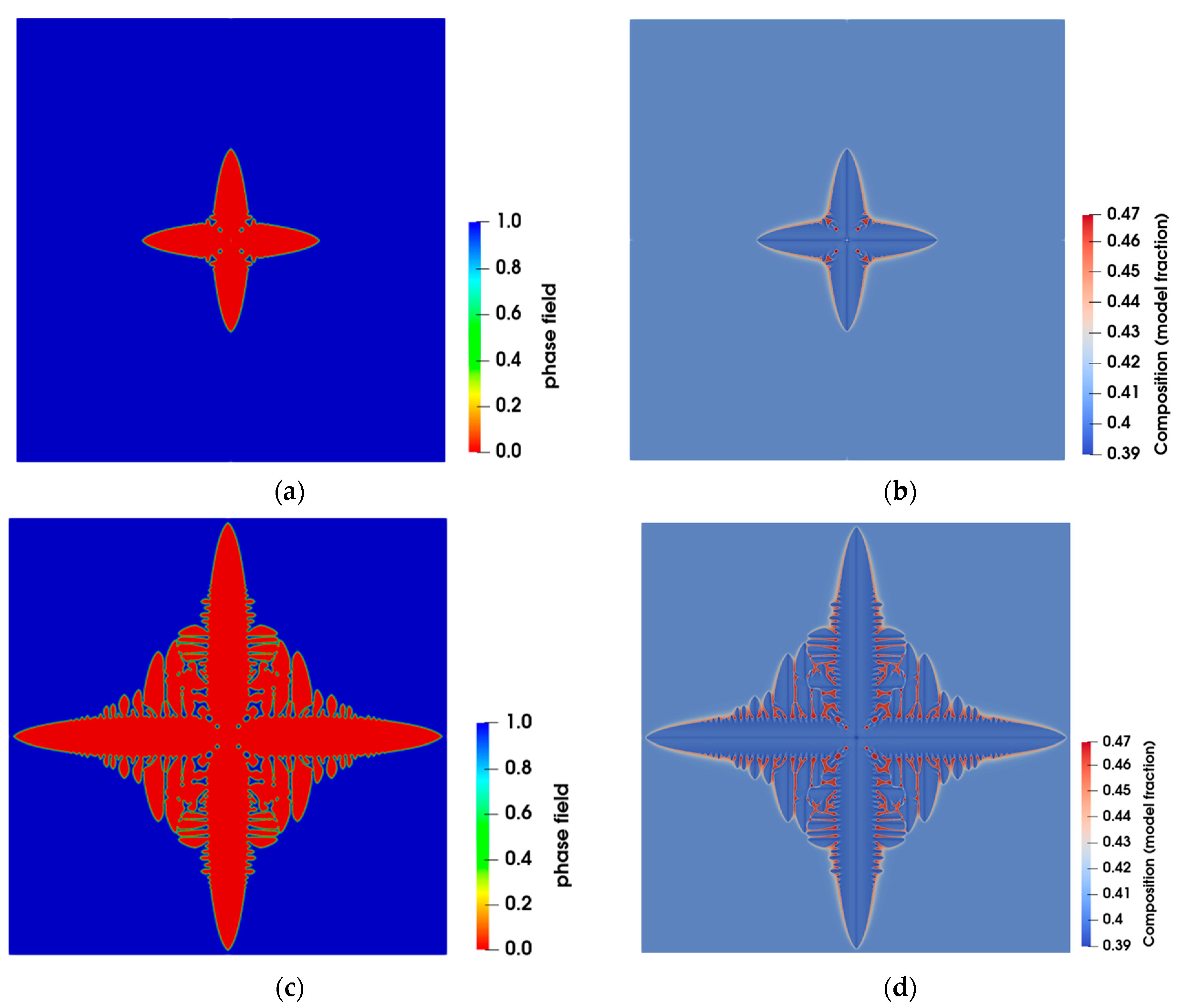
Figure 3.
Solute profile along the primary arm of the dendrite, at t = 2 ms, for Ni-Cu binary alloy.
Figure 3.
Solute profile along the primary arm of the dendrite, at t = 2 ms, for Ni-Cu binary alloy.
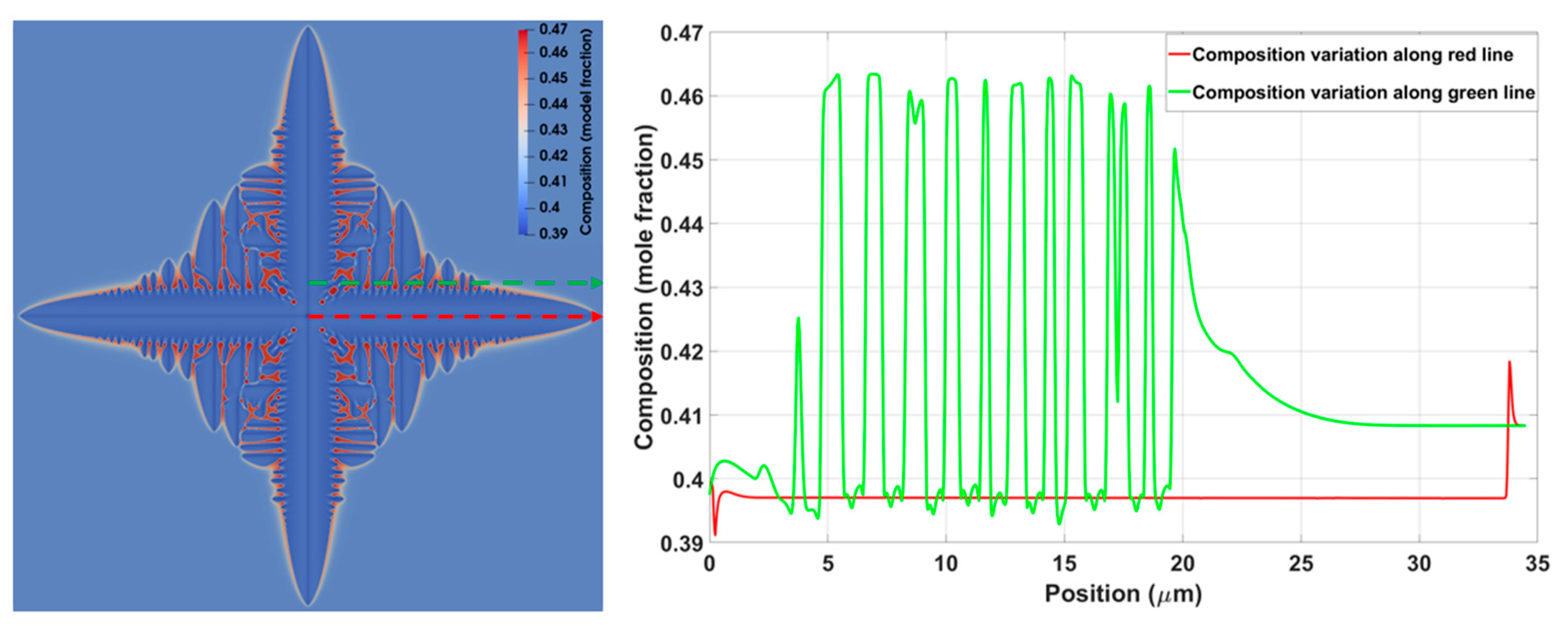
Figure 4.
Tip velocity of the equiaxed dendrite at different solidification times.

Figure 5.
Morphology of the dendrite (top) and composition (bottom) at t = 1.5 ms for Ni-Cu binary alloy in a computational domain of 23 μm 23 μm for different values of interface thickness (W).
Figure 5.
Morphology of the dendrite (top) and composition (bottom) at t = 1.5 ms for Ni-Cu binary alloy in a computational domain of 23 μm 23 μm for different values of interface thickness (W).

Figure 6.
Tip velocity of the equiaxed dendrite for different values of interface thickness (W).

Figure 7.
Solute profile along the primary stalk of the dendrite for different values of interface thickness (W) at t = 1.5 ms.
Figure 7.
Solute profile along the primary stalk of the dendrite for different values of interface thickness (W) at t = 1.5 ms.

Figure 8.
Growth morphology (top) and composition profile (bottom) at t = 2 ms in a computational domain of 34.5 μm 34.5 μm for different values of magnitude of anisotropy (δ).
Figure 8.
Growth morphology (top) and composition profile (bottom) at t = 2 ms in a computational domain of 34.5 μm 34.5 μm for different values of magnitude of anisotropy (δ).
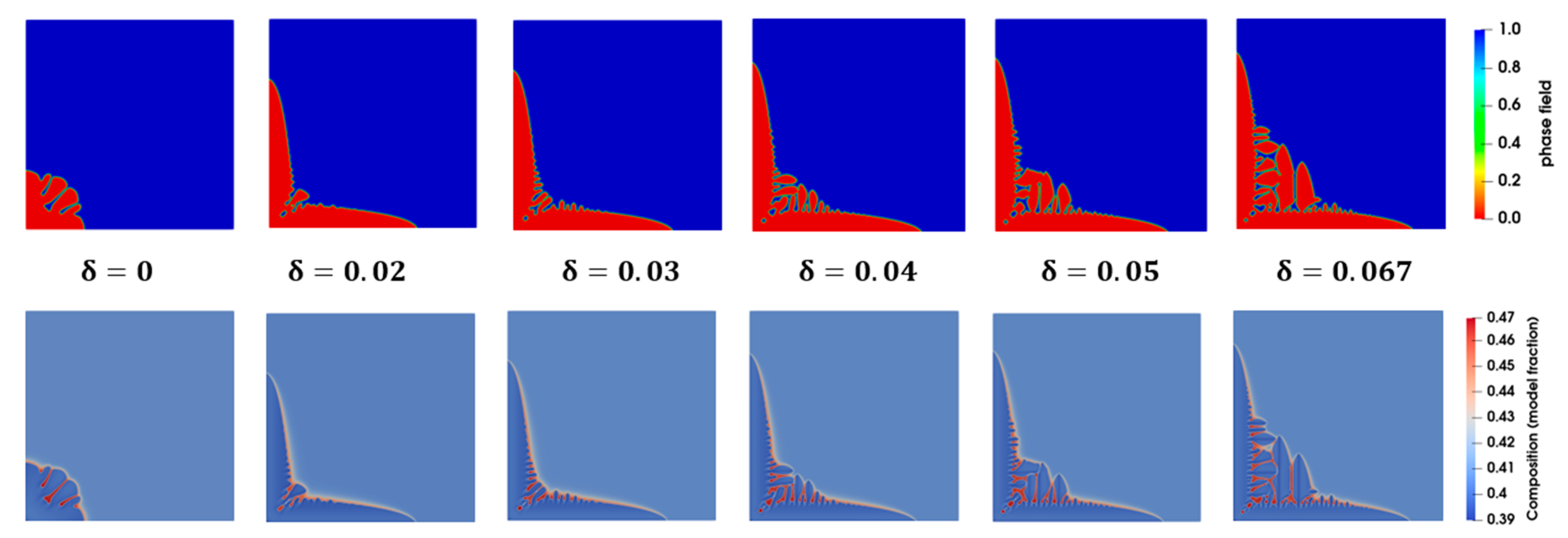
Figure 9.
Tip velocity of the dendrite vs. solidification time for different values of magnitude of anisotropy (δ).
Figure 9.
Tip velocity of the dendrite vs. solidification time for different values of magnitude of anisotropy (δ).
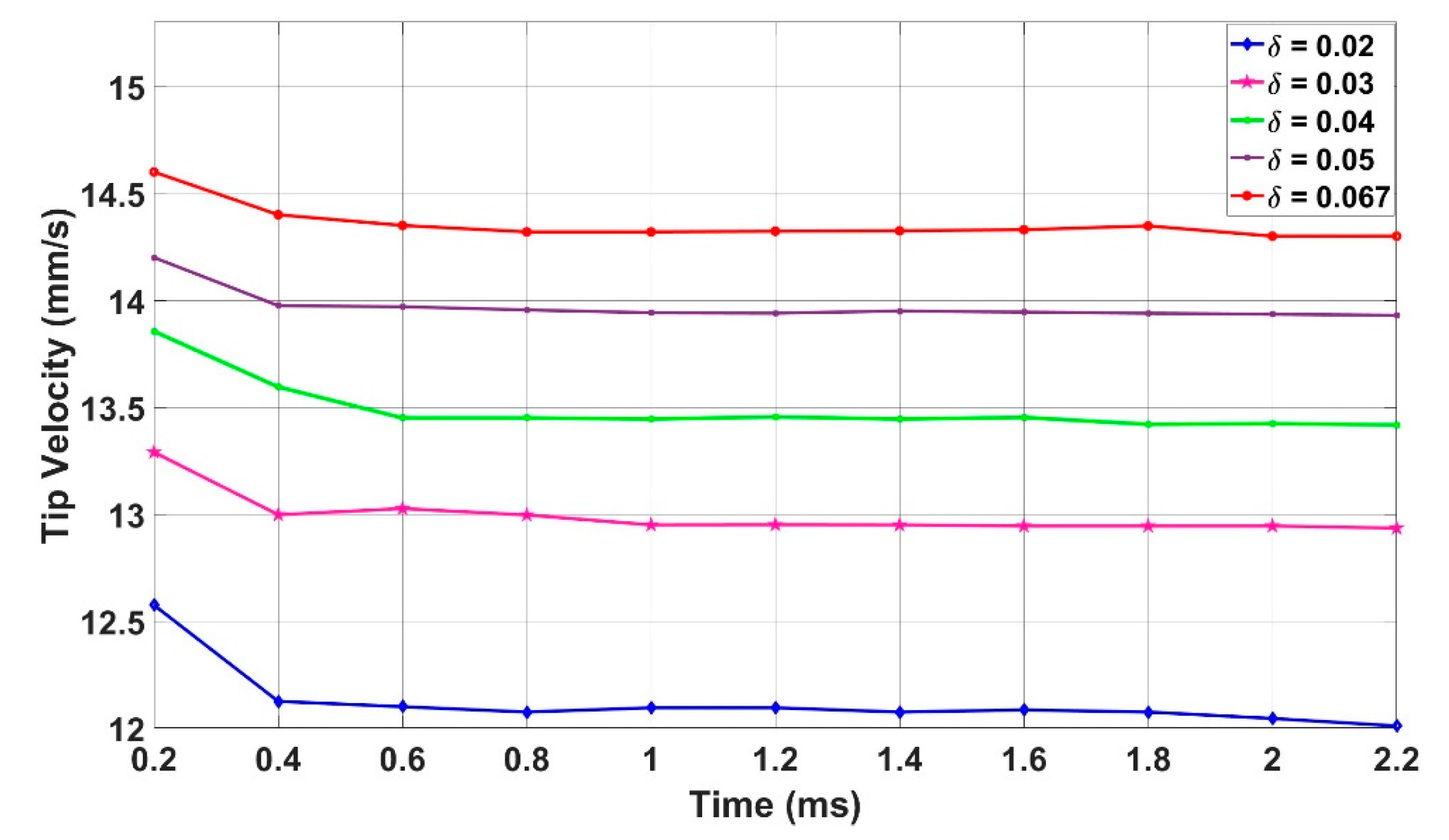
Figure 10.
Composition profile across the primary dendritic arm for different values of magnitude of anisotropy (δ) at t= 2 ms.
Figure 10.
Composition profile across the primary dendritic arm for different values of magnitude of anisotropy (δ) at t= 2 ms.

Figure 11.
Solute composition profile at t = 2.2 ms in a computational domain of 34.5 μm 34.5 μm for different values of antitrapping constant (a).
Figure 11.
Solute composition profile at t = 2.2 ms in a computational domain of 34.5 μm 34.5 μm for different values of antitrapping constant (a).
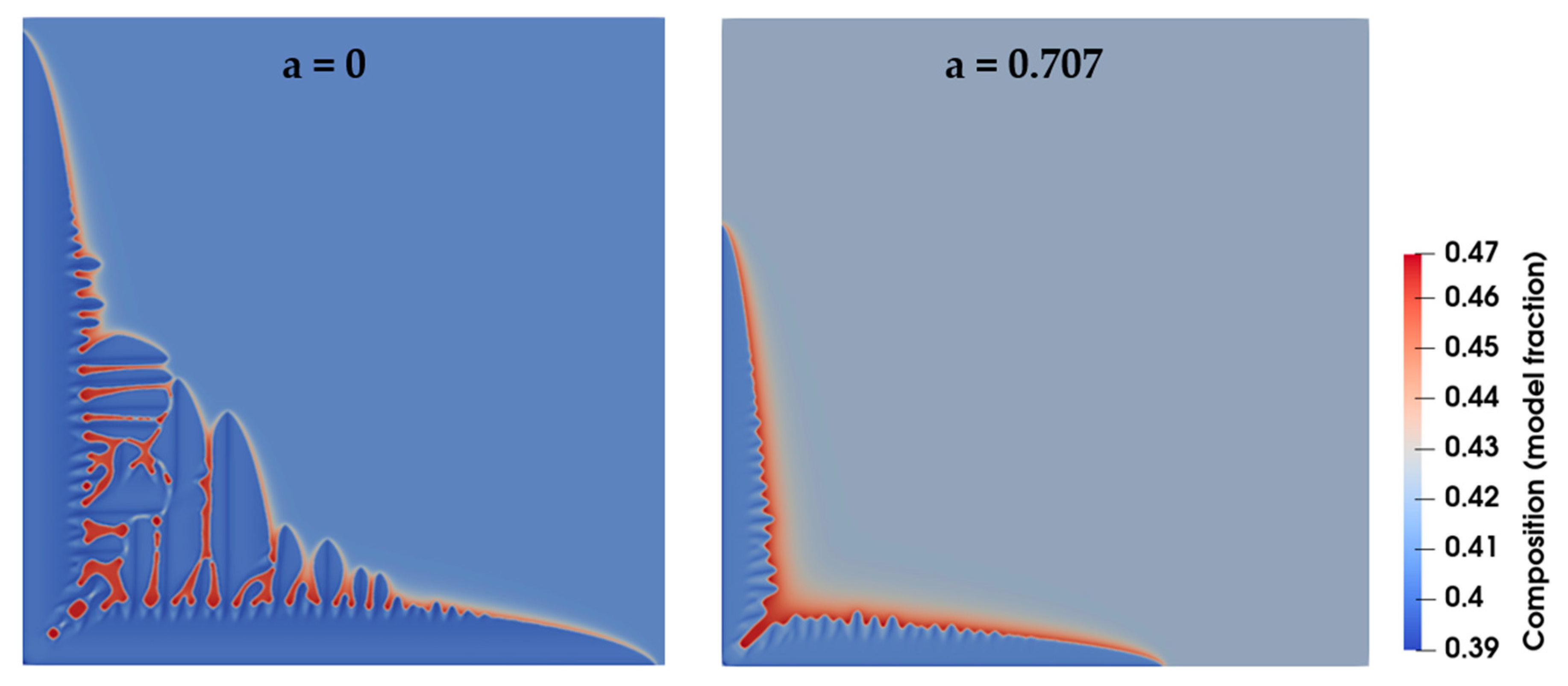
Figure 12.
Plot of composition along the primary dendrite arm at t = 2.2 ms in a computational domain of 34.5 μm × 34.5 μm for different values of antitrapping constant (a).
Figure 12.
Plot of composition along the primary dendrite arm at t = 2.2 ms in a computational domain of 34.5 μm × 34.5 μm for different values of antitrapping constant (a).
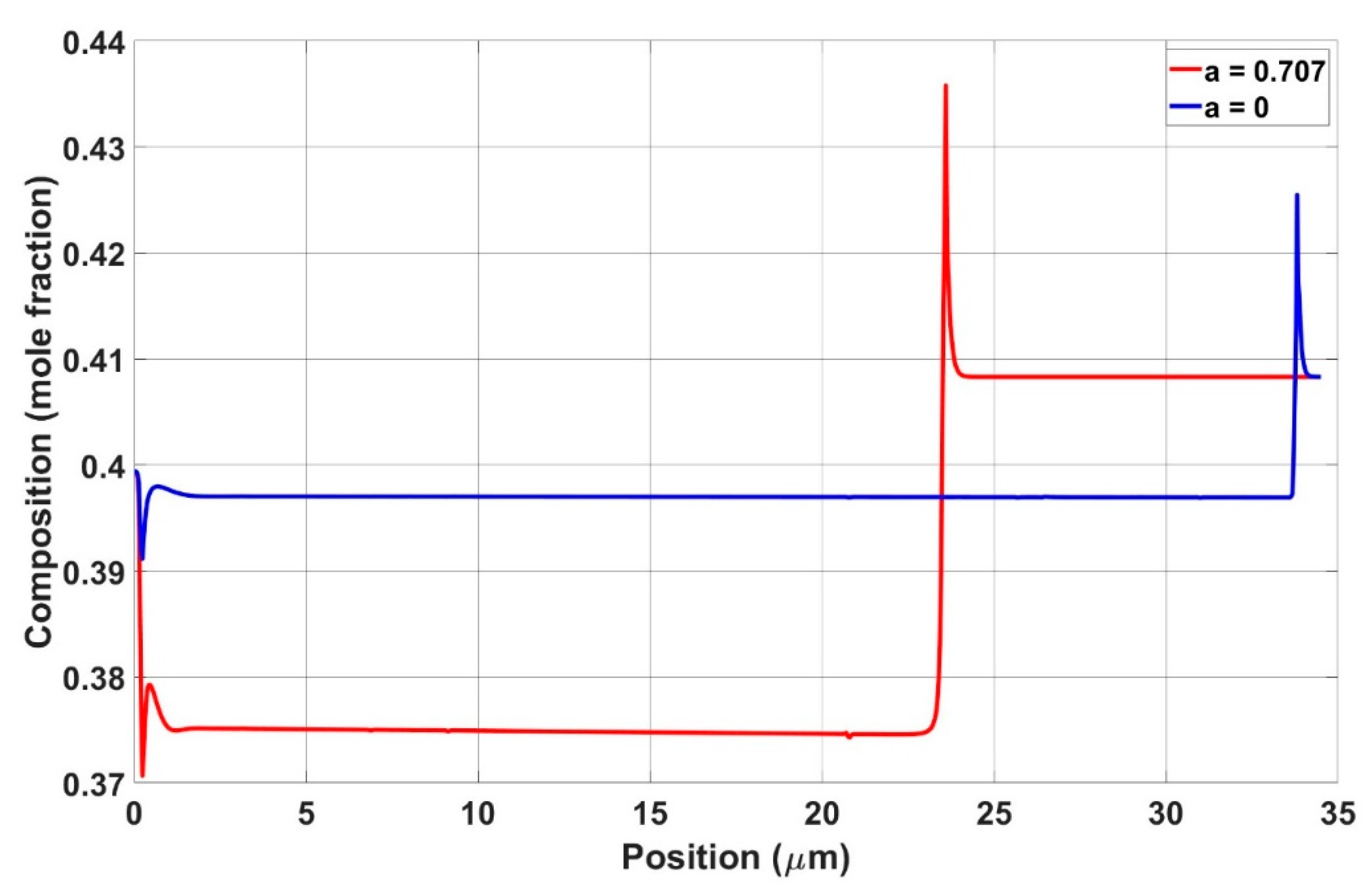
Figure 13.
Morphology of the dendrite (top) and composition profile (bottom) across the primary dendritic arm for different values of noise magnitude α after t = 2 ms.
Figure 13.
Morphology of the dendrite (top) and composition profile (bottom) across the primary dendritic arm for different values of noise magnitude α after t = 2 ms.
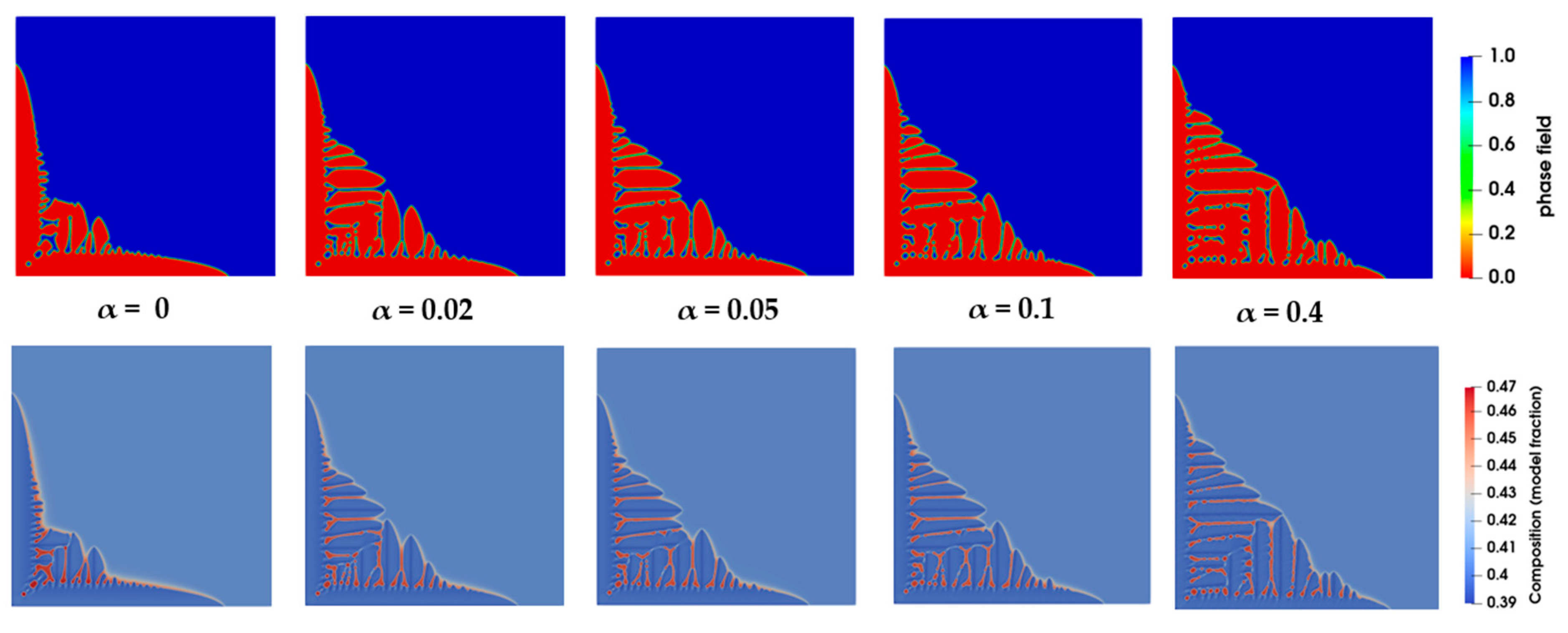
Figure 14.
(a) Solute composition profile along the primary dendrite at t = 2 ms and (b) tip velocity vs. time, for different values of amplitude of noise α.
Figure 14.
(a) Solute composition profile along the primary dendrite at t = 2 ms and (b) tip velocity vs. time, for different values of amplitude of noise α.

Figure 15.
Growth morphology of the dendrite under the influence of initial orientation at t = 1 ms in a computational domain of 34.5 μm × 34.5 μm.
Figure 15.
Growth morphology of the dendrite under the influence of initial orientation at t = 1 ms in a computational domain of 34.5 μm × 34.5 μm.

Figure 16.
Tip velocity of the dendrite vs. solidification time for different values of initial orientation ().
Figure 16.
Tip velocity of the dendrite vs. solidification time for different values of initial orientation ().
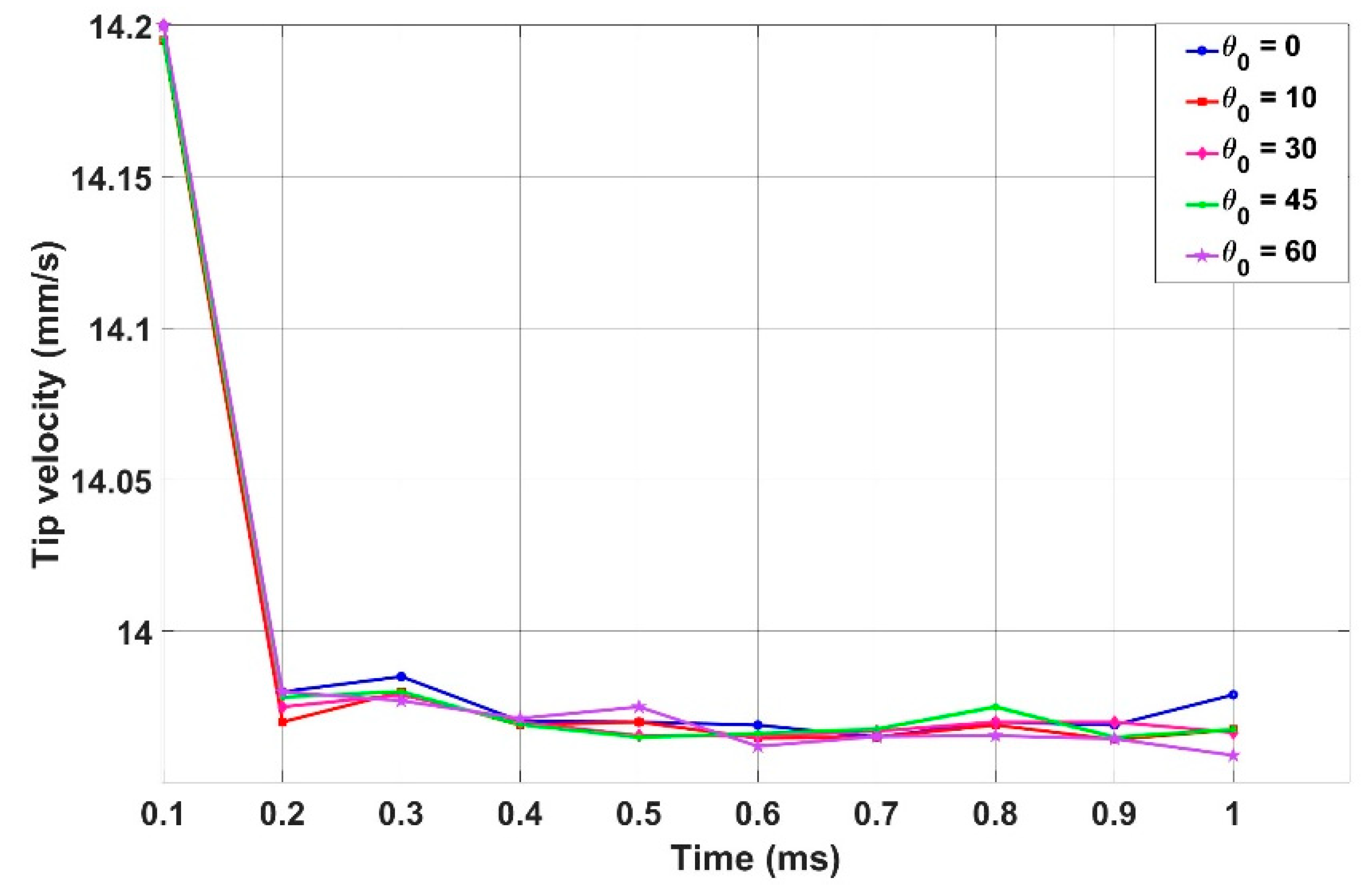
Figure 17.
Temperature variation across the computational domain for different values of thermal gradient G at t = 0.7 ms of the solidification time.
Figure 17.
Temperature variation across the computational domain for different values of thermal gradient G at t = 0.7 ms of the solidification time.

Figure 18.
Growth morphology (top) and composition profile (bottom) at t = 0.7 ms for different values of G in a computational domain of 34.5 μm 34.5 μm.
Figure 18.
Growth morphology (top) and composition profile (bottom) at t = 0.7 ms for different values of G in a computational domain of 34.5 μm 34.5 μm.

Figure 19.
Composition profile across the primary dendritic arm for different G values at t = 0.7 ms. The nucleus is at the center for all cases.
Figure 19.
Composition profile across the primary dendritic arm for different G values at t = 0.7 ms. The nucleus is at the center for all cases.
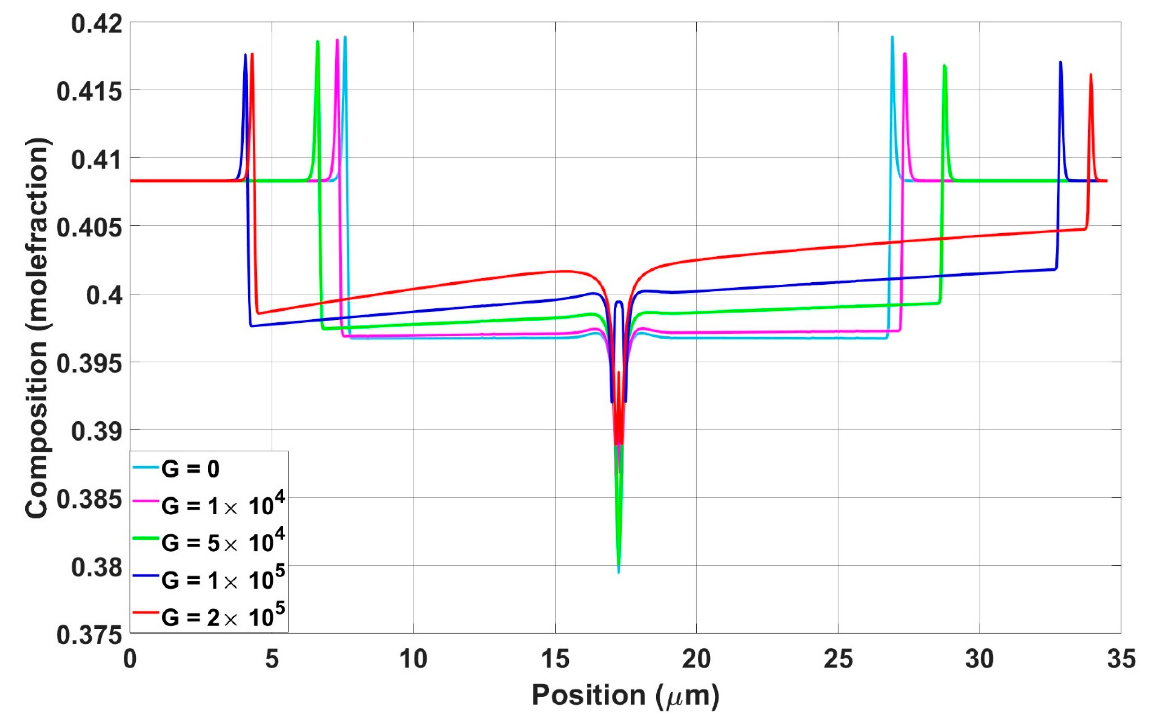
Figure 20.
Composition profiles after different times (a) 1 ms, (b) 2 ms, and (c) 3 ms and orientation fields (d) 1 ms, (e) 2 ms, and (f) 3 ms for polycrystalline growth on a 2D computational domain of length 69 μm 69 μm.
Figure 20.
Composition profiles after different times (a) 1 ms, (b) 2 ms, and (c) 3 ms and orientation fields (d) 1 ms, (e) 2 ms, and (f) 3 ms for polycrystalline growth on a 2D computational domain of length 69 μm 69 μm.
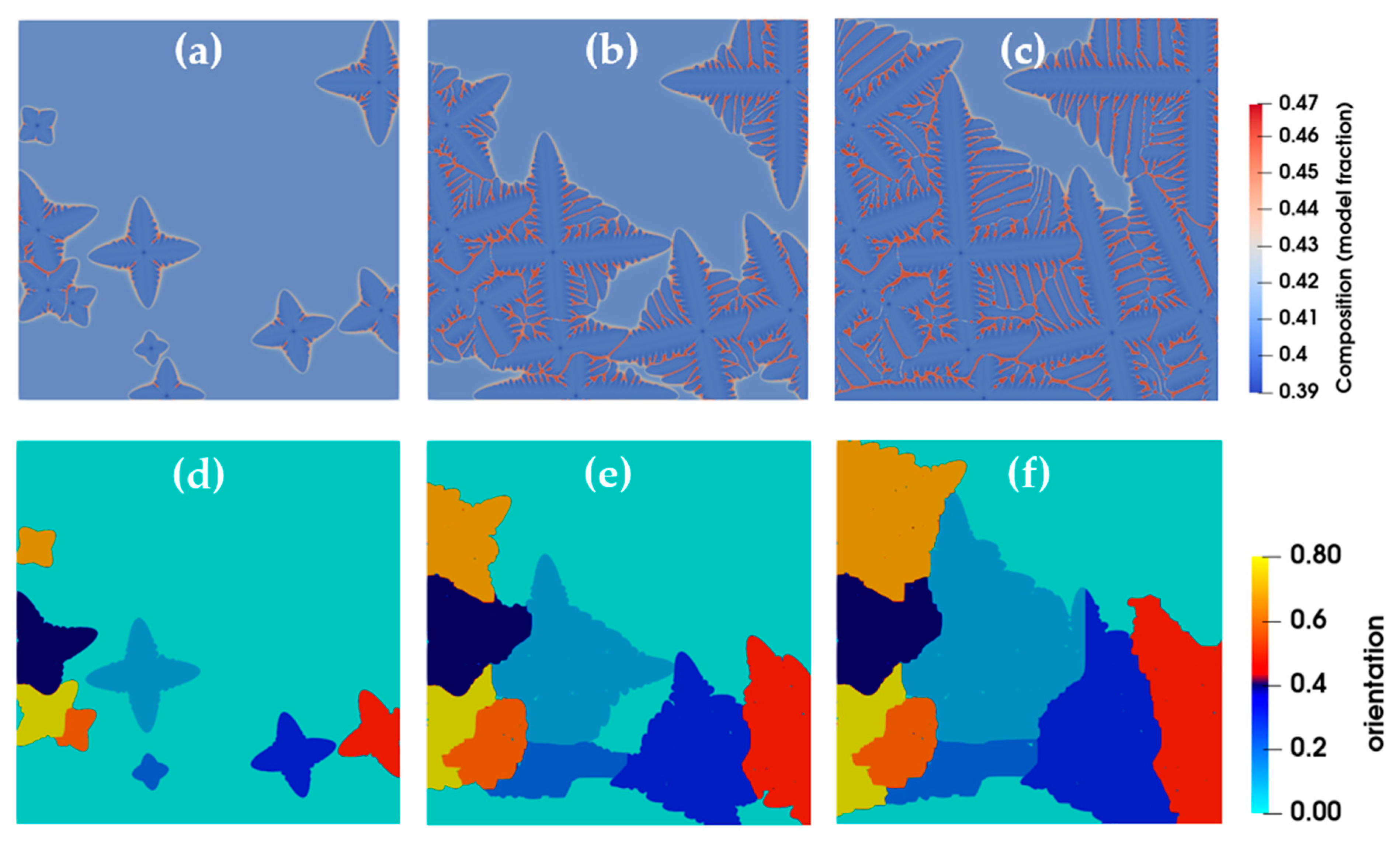
Figure 21.
Composition profiles at t = 3 ms, along a central axis parallel to the X-axis.


Table 1.
Empirical relations to calculate the computational parameters [25].
Table 1.
Empirical relations to calculate the computational parameters [25].
| = | = |
| = | = |
| = = | |
Table 2.
Normalized growth driving force, Peclet number, and the solute partition coefficient (k) at different values of W; keq is the equilibrium partition coefficient.
Table 2.
Normalized growth driving force, Peclet number, and the solute partition coefficient (k) at different values of W; keq is the equilibrium partition coefficient.
| Interface Thickness (W) (nm) | (Mole Fraction) | (Mole Fraction) | Vtip (mm/s) | Tip Radius () (mm) | |||||
|---|---|---|---|---|---|---|---|---|---|
| 73.4 | 0.39821 | 0.42551 | 0.58419 | 0.942 | 13.98 | 0.194 | 1.246 | 0.794 | 0.8556 |
| 48.9 | 0.396929 | 0.41835 | 0.468699 | 0.948796 | 13.6 | 0.178 | 1.19 | 0.787 | 0.8556 |
| 32.6 | 0.3952 | 0.4216 | 0.503409 | 0.937381 | 14 | 0.114 | 0.73 | 0.73 | 0.8556 |
| 24.5 | 0.39396 | 0.42356 | 0.515203 | 0.930116 | 13.985 | 0.109 | 0.58 | 0.72 | 0.8556 |
| 19.56 | 0.392679 | 0.4251 | 0.517874 | 0.923733 | 13.99 | 0.11 | 0.52 | 0.718 | 0.8556 |
Table 3.
Comparative analysis of normalized growth driving force and the solute partition coefficient (k) at varying antitrapping constant values, compared with data from Lan and Shih [33].
Table 3.
Comparative analysis of normalized growth driving force and the solute partition coefficient (k) at varying antitrapping constant values, compared with data from Lan and Shih [33].
| Antitrapping Constant (a) | (Mole Fraction) | (Mole Fraction) | Vtip (mm/s) | Tip Radius () (μm) | [33] | Vtip [33] (mm/s) | Tip Radius () (μm) [33] | k [33] | ||
|---|---|---|---|---|---|---|---|---|---|---|
| 0 | 0.39821 | 0.42551 | 0.58419 | 14 | 0.178 | 0.593 | 14.2 | 0.942 | 0.178 | 0.943 |
| 0.707 | 0.37921 | 0.43752 | 0.49897 | 10.76 | 0.11 | 0.492 | 10.85 | 0.866 | 0.112 | 0.888 |
Disclaimer/Publisher’s Note: The statements, opinions and data contained in all publications are solely those of the individual author(s) and contributor(s) and not of MDPI and/or the editor(s). MDPI and/or the editor(s) disclaim responsibility for any injury to people or property resulting from any ideas, methods, instructions or products referred to in the content. |
© 2023 by the authors. Licensee MDPI, Basel, Switzerland. This article is an open access article distributed under the terms and conditions of the Creative Commons Attribution (CC BY) license (https://creativecommons.org/licenses/by/4.0/).
Share and Cite
MDPI and ACS Style
Al Azad, A.R.; Cardiff, P.; Browne, D.J. Development and Numerical Testing of a Model of Equiaxed Alloy Solidification Using a Phase Field Formulation. Metals 2023, 13, 1916. https://doi.org/10.3390/met13121916
AMA Style
Al Azad AR, Cardiff P, Browne DJ. Development and Numerical Testing of a Model of Equiaxed Alloy Solidification Using a Phase Field Formulation. Metals. 2023; 13(12):1916. https://doi.org/10.3390/met13121916
Chicago/Turabian StyleAl Azad, Abdur Rahman, Philip Cardiff, and David J. Browne. 2023. "Development and Numerical Testing of a Model of Equiaxed Alloy Solidification Using a Phase Field Formulation" Metals 13, no. 12: 1916. https://doi.org/10.3390/met13121916
Note that from the first issue of 2016, this journal uses article numbers instead of page numbers. See further details here.