Article

Calculation and Analysis of Equilibrium Position of Aerostatic Bearings Based on Bivariate Interpolation Method

1
School of Mechatronics Engineering, Zhongyuan University of Technology, Zhengzhou 451191, China
2
Faculty of Mechanical and Electrical Engineering, Kunming University of Science and Technology, Kunming 650500, China
*
Author to whom correspondence should be addressed.
Lubricants 2024, 12(3), 85; https://doi.org/10.3390/lubricants12030085
Submission received: 22 January 2024 / Revised: 17 February 2024 / Accepted: 5 March 2024 / Published: 7 March 2024
(This article belongs to the Special Issue Tribological Characteristics of Bearing System, 2nd Edition)

Abstract

:
The solution of equilibrium positions is a critical component in the calculation of the dynamic characteristic coefficients of aerostatic bearings. The movement of the rotor in one direction leads to bidirectional variations in the air film force, resulting in low efficiency when using conventional calculation methods. It can even lead to iterative divergence if the initial value is improperly selected. This study concentrates on the orifice throttling aerostatic bearings and proposes a novel method called the bivariate interpolation method (BIM) to calculate the equilibrium position. The equilibrium equation for the rotor under the combined influence of air film forces, gravity, and external loads is established. A calculation program based on the finite difference method is developed to determine the equilibrium position. The process of solving the equilibrium position and the convergence is compared with the secant method and the search method. Furthermore, the variation trend of the equilibrium position and stiffness when the external loads changes are studied based on the BIM. Finally, the correctness of the BIM to solve the equilibrium position is proved by comparing it with the experiment results. The calculation results indicate that the BIM successfully resolves the problem of initial value selection and exhibits superior computational efficiency and accuracy. The equilibrium position initially moves away from the direction of the external load as the load increases, and then this gradually approaches the load direction. The main stiffness increases with increases in the external load, while the variation in cross stiffness depends on the direction of the external load.

1. Introduction

Aerostatic bearings utilize compressed air from external air sources to form an air film that supports the movement of the parts. Compared to precision rolling bearings, aerostatic bearings offer significant advantages in terms of motion accuracy, friction, rotation speed, and environmental impact [1]. Consequently, aerostatic bearings have found widespread applications in aerospace, precision machine tools, electronics and semiconductors, and medical equipment [2,3,4]. Commonly used orifice throttling aerostatic bearings materials are steel, brass, and aluminum [5]. In addition, porous materials also have more applications because of their superior characteristics [6], and the commonly used material is graphite. Research on aerostatic bearings primarily focuses on topics such as bearing capacity, stiffness, stability, and flow rate [7,8]. The equilibrium position is an important basis for judging the stability of aerostatic bearings [9], and it is also the premise of analyzing the dynamic characteristic coefficients of aerostatic bearings under normal operation. While the static load of practical bearings is typically known, the equilibrium position remains unknown [10]. The accurate and efficient solution of the equilibrium position of a bearing under a given load is a necessary prerequisite for studying the relevant characteristics of aerostatic bearings.
Solving the Reynolds equation is the first step to study the relevant characteristics of aerostatic bearings, which can be divided into the finite difference method (FDM), the finite element method (FEM), and the finite volume method (FVM) according to different solving methods [11]. Due to the nonlinearity of the equilibrium equation, multiple iterations are necessary to determine the equilibrium position of the bearing. Scholars have proposed numerical calculation methods to solve the equilibrium position of the rotor. Shuai [12] used the coordinate rotation method to solve the equilibrium position of the three-lobe journal bearing and proved the feasibility of the numerical calculation method to solve the equilibrium position of the three-lobe journal bearing. However, this method is not suitable for the cylindrical sliding bearing. Qian [13] determined the equilibrium position of the three-lobe journal bearing using the secant method. Wang [14] analyzed the influence of unbalance force on the vibration characteristics of the narrow slit throttling aerostatic bearing and observed that as the speed increases, the rotor’s equilibrium position gradually moves towards the center of the bearing. However, no detailed method was provided for solving the equilibrium position. Yu [15] used the search method to solve the equilibrium position of the tilting pad journal bearing. By calculating the direction of the fastest convergence of the air film force based on a given trial calculation point, the equilibrium position of the bearing can be obtained. Results show that the method effectively solves the divergence problem, although its calculation efficiency is low due to the frequent calculation of the air film force. Wan [16] used the Newton iteration method to solve the equilibrium position of the bearing and proposed a load approaching method to solve the problem of the Newton iteration method, getting stuck in a dead loop due to inappropriate initial value selection. Zheng [17] used the fast convergence speed of the Newton–Raphson method to solve the equilibrium position of the bearing and subsequently determined the dynamic characteristic coefficients. The accuracy of the method was proven by comparing it with relevant references. Pokorny [18] optimized the Newton iteration method and compared it with the Newton–Raphson method. The equilibrium position of the tilting pad bearing was then determined, demonstrating the superiority of the optimized Newton method over the Newton–Raphson method. Yang [19] has demonstrated through numerical analysis that the twofold secant method converges faster than both Newton’s method and Newton’s method with the P.C. format. Zhou [20] used the twofold secant method to solve the static equilibrium position. The results show that the twofold secant method significantly narrows down the search range in the initial iteration and achieves faster convergence compared to the dichotomy method and the secant method. All of the aforementioned methods for solving the equilibrium position used the static Reynolds equation. Furthermore, the dynamic trajectory method can be employed to determine the equilibrium position, although it often necessitates two to three days to ensure accurate calculations, making it relatively time-consuming [21].
When the rotor is in a stable state, the dynamic characteristic coefficients of the bearing during normal operation can be solved and analyzed. The methods for solving the dynamic characteristic coefficients of the bearing include the difference method, the partial derivative method, the small parameter method, and the finite element method [22,23,24,25]. Meng [26] used the difference method to solve the stiffness of the oil-lubricated journal bearing and analyzed the influence of bearing parameters. The accuracy of the calculated values was proved by comparing the theoretical calculation values with the experimental data. Qi [27] used the partial derivative method to solve the Reynolds equation defined in the complex range and focused on investigating the effect of rotor disturbance frequency on stiffness and damping coefficients. Li [28] solved the Reynolds equation using the partial derivative method. The calculation results indicate that as the rotor position gradually approaches the equilibrium position, the dynamic characteristic coefficients gradually converge to a stable value.
In summary, many existing references calculate bearing-related characteristics using a fixed eccentricity, but there is a lack of research on solving the equilibrium position and conducting characteristic analysis under given loads. The current methods for solving the equilibrium position are primarily used for the liquid sliding bearing, and varying levels of efficiency and convergence problems exist. This paper focuses on the orifice throttling radial aerostatic bearing as the subject of research and presents a new method, called the BIM, for determining the equilibrium position. The influence of external load on the equilibrium position and dynamic characteristic coefficients is studied, and the calculation results are discussed and compared with references and experimental data.

2. Building and Calculation of the BIM

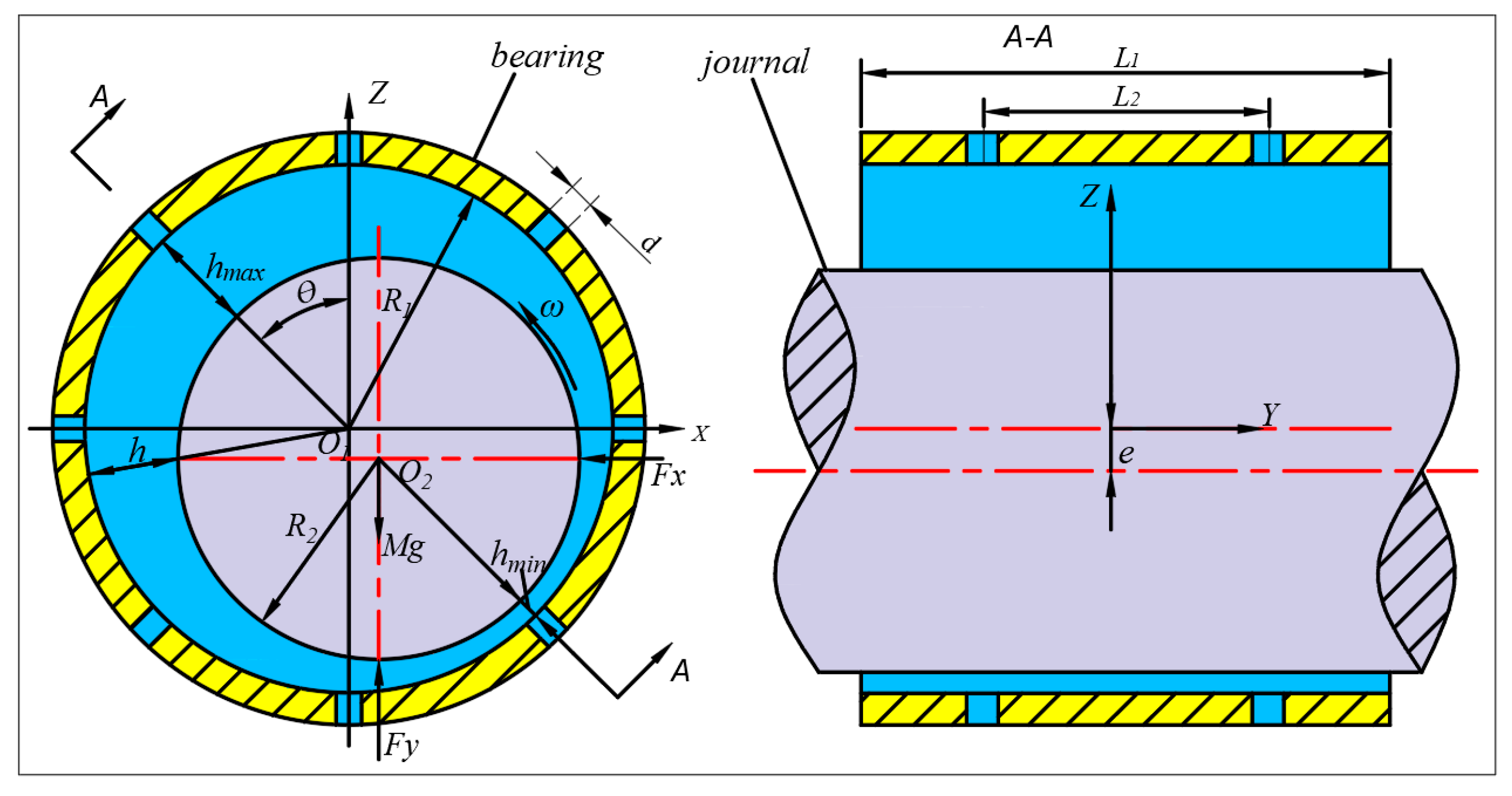
2.1. Establishment of Mathematical Model of Bearing

Figure 1 depicts the structural model of the orifice throttling aerostatic bearing studied in this paper. Table 1 provides the fundamental parameters of the bearing. O 1 is the center of the bearing, and O 2 is the center of the journal. When there are no external loads present, the rotor experiences air film forces F x and F y , in addition to its own weight M g , at the equilibrium position.
To determine the capacity of the aerostatic bearing, it is necessary to first obtain the air film pressure distribution of the bearing. The bearing is at the equilibrium position, with a stable air film pressure distribution. Because the influence of temperature on aerostatic bearing is revlatively small, the flow process duration is short, so it can be isothermal flow [29]. The commonly used Reynolds equation for compressible gas lubrication can be expressed as
x P h 3 P x + y P h 3 P y + Q δ = 6 μ U P h x
The air film thickness can be expressed as h = c ( 1 + ε cos θ ) , where ε is the eccentricity, and θ is the attitude angle.
It is noted that δ k = 1 at the orifice entrance, and that δ k = 0 at the orifice exit. Q is the air mass flow factor:
Q = 12 μ P a ρ a ρ υ
Orifice flow equation:
m = φ P s A 2 ρ a P a ψ = ρ υ d x d y
and
ψ = K 2 2 K + 1 K + 1 K 1 0.5 , P P s β k K K 1 P P s 2 K P P s K + 1 K 0.5 , P P s > β k
where φ is the flow coefficient, A is the restriction area, K is the air constant, and β k is the critical pressure ratio.
By utilizing the FDM to solve Equation (1), the air film pressure can be determined for a given rotor position. Then, integrating the air film pressure using Equation (5) yields the horizontal and vertical air film forces of the bearing.
F x = 0 L 0 2 π P R sin θ d θ d y F y = 0 L 0 2 π P R cos θ d θ d y
Assuming that the initial position of the rotor is vertically oriented, as shown in Figure 2a, the rotor is then horizontally displaced by a distance of + Δ x , resulting in the position shown in Figure 2b. The horizontal movement causes a change in the attitude angle θ , subsequently impacting the distribution of the air film pressure P . According to Equation (5), both the horizontal and vertical bearing capacity are consequently altered.

2.2. Mathematical Model of the BIM

During the motion of the rotor, irrespective of the effects of other factors, the rotor is affected by the combined action of the air film force of the bearing and the gravity of the rotor. When the rotor reaches an equilibrium position, Equation (6) need to be satisfied.
F X = F x = 0 F Y = F y M g = 0
When solving the equilibrium position using the secant method and the Newton method, the horizontal and vertical coordinates are successively iterated in one direction, as shown in Figure 3. When solving the process, the iterative process of abscissa is embedded in the iterative process for the ordinate. The correction of the ordinate can only begin once the horizontal bearing capacity satisfies the requirements. It can be seen from Figure 2 that the movement of the rotor in one direction causes the bidirectional variations in the air film force. Therefore, there are the following problems:
(1)
After completing a calculation in the vertical direction, the horizontal bearing capacity fails to satisfy the convergence requirements, necessitating a recalculation of the abscissa. Therefore, until the ordinate satisfies the convergence requirements, each correction of the ordinate requires iterative adjustments of the abscissa. This process results in a reduction in computational efficiency.
(2)
In the iterative calculation process, it is essential to determine the influence factors. Influence factors are used to correct the coordinates. The influence factors vary depending on the rotor’s position. If the influence factors are excessively large, it can result in iterative divergence, whereas if they are excessively small, it can impact computational efficiency.
Figure 3. Common methods to solve the process.
Lubricants 12 00085 g003
The proposed BIM in this paper takes into account the simultaneous effect of horizontal and vertical coordinates on the air film force. There are relationships between the position to be solved and the four known positions surrounding it. Subsequently, the unknown position is determined through two consecutive interpolation steps. Figure 4 illustrates the principle diagram of the BIM, while Equation (7) represents the interpolation equation.
F = a x + b y + c x y + d
The coefficient a controls the coordinate x. The abscissa x of the equilibrium position can be corrected by adjusting a. The coefficient b controls the coordinate y. The ordinate y of the equilibrium position can be corrected by adjusting b. The coefficient c controls the cross-term between the coordinates x and y and describes the interaction relationship between the horizontal and vertical coordinates. It can adjust the iteration direction. The coefficient d is a constant term used to adjust the overall offset of the function.
The interpolation conditions are as follows:
F x ( x 1 , y 1 ) = F x 1 , F y ( x 1 , y 1 ) = F y 1 F x ( x 2 , y 1 ) = F x 2 , F y ( x 2 , y 1 ) = F y 2 F x ( x 2 , y 2 ) = F x 3 , F y ( x 2 , y 2 ) = F y 3 F x ( x 1 , y 2 ) = F x 4 , F y ( x 1 , y 2 ) = F y 4
To determine the equilibrium position and account for the impact of rotor position changes on the horizontal and vertical air film forces, the interpolation equation can be simplified to Equation (8) by using the interpolation conditions, where F x l o a d and F y l o a d represent the magnitude of the external load applied in the respective horizontal and vertical directions.
F x l o a d = F x 1 1 u 1 v + F x 2 u 1 v + F x 3 u v + F x 4 1 u v F y l o a d = F y 1 1 u 1 v + F y 2 u 1 v + F y 3 u v + F y 4 1 u v
where
u = x x 1 x 2 x 1 ,   v = y y 1 y 2 y 1
During the iterative calculation process, it is necessary to determine the modified coordinate value based on the magnitudes of the influence factors a and b . If a > b , the abscissa x is corrected; otherwise, the ordinate y is corrected. Adjusting the coordinates based on the influence factors helps prevent incorrect iteration direction and improves computational efficiency. By combining Equations (7) and (8), the influence factors a and b are obtained.
a = y 2 ( F y 2 F y 1 ) + y 1 ( F y 4 F y 3 ) ( x 2 x 1 ) ( y 2 y 1 ) , b = x 1 ( F y 2 F y 1 ) + x 2 ( F y 4 F y 3 ) ( x 2 x 1 ) ( y 2 y 1 )

2.3. Calculation Process of the BIM

Figure 5 illustrates the flowchart of the BIM used to calculate the equilibrium position of the bearing. The bearing capacity is determined through the Reynolds equation. The database is used to temporarily store and transfer data between the journal position obtained through the BIM and the bearing capacity calculated through the Reynolds equation.
The iterative process is as follows:
(1)
Given convergence criteria (resultant force | F X | < 10 3 N, | F Y | < 10 3 N, 0.001 N force can be ignored).
(2)
According to Figure 4, four points ( x 1 , y 1 ) , ( x 2 , y 1 ) , ( x 2 , y 2 ) , ( x 1 , y 2 ) in the bearing range are selected, and u , v are calculated.
(3)
The air film forces ( F x 1 , F y 1 ) , ( F x 2 , F y 2 ) , ( F x 3 , F y 3 ) , ( F x 4 , F y 4 ) at the corresponding positions were calculated by the Reynolds equation.
(4)
Through Equation (8), coordinate points ( x , y ) are obtained after two consecutive interpolation calculations.
(5)
The air film forces ( F x , F y ) at the position of the fourth step are obtained by the Reynolds equation and compared with the convergence condition. If it is satisfied, the iteration is terminated. If it is not satisfied, proceed to step 6.
(6)
Determine the size of the impact factors a and b and determine the coordinate value that has the greatest influence on the air film force. If a > b , modify x ; otherwise, modify y . Repeat steps 2 to 5 after updating the data.

3. Results and Discussion

3.1. Comparison of Different Methods

Figure 6 illustrates the iterative convergence process of the BIM, the secant method, and the search method for solving the bearing equilibrium position under the same parameters. It can be observed from Figure 6 that the equilibrium positions obtained by the three methods are almost coincident. The main reason is that different calculation methods have different convergence. The convergence condition of the secant method is F < 1 × 10 2 N, the search method is F < 5 × 10 2 N, and the BIM is F < 1 × 10 3 N. The BIM exhibits the highest calculation accuracy. When compared with the secant method, the BIM has errors of 0.03% and 0.02% in the horizontal and vertical coordinates of the equilibrium position, respectively. When compared with the search method, the BIM has errors of 0.15% and 0.06% in the horizontal and vertical coordinates of the equilibrium position, respectively. The maximum error is 0.15%, while the minimum error is 0.02%. Table 2 provides a comparison of the results obtained using the three methods. The BIM requires 4 iterations, the secant method requires 22 iterations, and the search method requires 15 iterations. The BIM exhibits superior calculation efficiency compared with the other methods. In the initial iteration calculation, the convergence curve experiences substantial variations due to the significant initial distance from the equilibrium point. The convergence speed gradually slows down after approaching the equilibrium point. The secant method exhibits poor convergence performance near the equilibrium position due to the high density of points, resulting in reduced calculation efficiency.

3.2. Calculation of Equilibrium Position Based on the BIM

The equilibrium position in this study is primarily influenced by the air film pressure, which is closely associated with the supply pressure and rotor speed. Figure 7a illustrates the variations in the equilibrium position as the supply pressure and rotational speed. As shown in Figure 7a, the equilibrium position gradually moves towards the center of the bearing with increasing rotational speed and supply pressure. This rule is consistent with the results of reference [8].
Taking a speed of 5000 r/min and a supply pressure of 0.5 MPa as an example, the variation in the equilibrium position is shown in Figure 7b when the horizontal force F x and the vertical force F y ranging from −1200 N to 1200 N with an increment of 100 N are applied to the rotor. When subjected to external loads, the eccentricity ε gradually increases, and the equilibrium position of the axis will first move away from the load direction. As the absolute value of the external load increases, the equilibrium position progressively aligns with the direction of the external load, while the extent of the change decreases.

3.3. Calculation of Stiffness of Equilibrium Position Based on the BIM

The stiffness of aerostatic bearing is solved by the difference method. After obtaining the equilibrium position, a horizontal disturbance + Δ x is applied at the equilibrium position, and the air film forces F x 1 and F y 1 are solved under the new geometric relationship. Similarly, the disturbance Δ x is taken, and F x 2 , F y 2 can be obtained. Then, the stiffness values are then obtained as Kxx and Kyx.
K x x = F x 1 F x 2 2 Δ x
K y x = F y 1 F y 2 2 Δ x
Similarly, the stiffness values Kxy, Kyy can be obtained by adding disturbance + Δ y and Δ y in the vertical direction.
K x y = F x 3 F x 4 2 Δ y
K y y = F y 3 F y 4 2 Δ y
Figure 8 illustrates that the direct stiffness and the absolute values of cross stiffness at the equilibrium position gradually rise with increasing rotational speed and supply pressure. Moreover, stiffness values are more responsive to changes in rotational speed. This phenomenon can be attributed to the growing dynamic pressure effect of the bearing as the rotational speed increases, leading to an overall increase in stiffness. The main stiffness Kxx is approximately equal to Kyy, and the cross stiffness Kxy is approximately inversely proportional to Kyx. This rule is consistent with the conclusion of reference [16].
The increase in both rotational speed and supply pressure leads to an increase in air film stiffness. The change in rotational speed has a greater influence on stiffness compared to supply pressure. This also explains that the influence of rotational speed on the change in the equilibrium position in Figure 7a is greater than that of supply pressure. With the increase in both speed and supply pressure, the equilibrium position shifts towards the center of the bearing.
Figure 9a,b illustrate the variations in stiffness at the equilibrium position caused by the external loads F x and F y . The direct stiffness increases as the absolute value of the external load increases, while the variation in cross stiffness depends on the direction of the applied load. If the absolute value of the external load F x increases gradually, the corresponding Kxy increases, while the absolute value of Kyx decreases. If the absolute value of the external load F y increases gradually, the corresponding Kxy decreases, while the absolute value of Kyx increases. This can also explain the trend observed in Figure 7b regarding the influence of external loads on the change in equilibrium position.

4. Experiments and Comparison

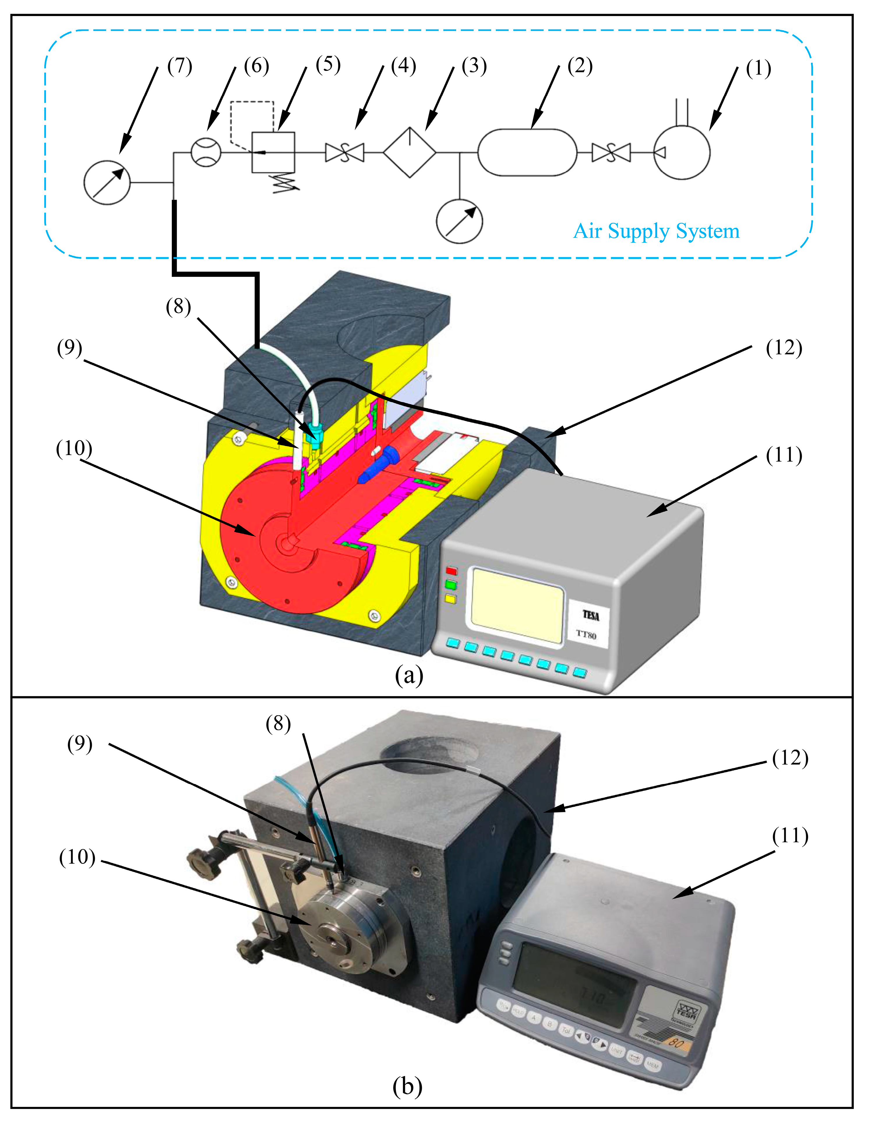
4.1. Introduction of Experimental Platform

Figure 10 shows the experiment setup used to measure the equilibrium position, comprising the air supply system, the tested motorized spindle, and the TESA TT80 inductance micrometer. The air supply system is constructed by an air compressor (1), filter (3), globe value (4), solenoid throttle value (5), flowmeter (6), and pressure gauge (7). The inductance micrometer (accuracy 10 nm, range ±5 μm) is constructed with an inductive probe (9) and a digital display unit (11). The rotor diameter is measured with the Mitutoyo MDE-75MX (resolution 0.001 mm, allowable error 2 μm), while the bearing diameter is measured with the Mitutoyo CG-D100 (resolution 0.001 mm, allowable error 3 μm). Table 3 gives three sets of measured data, with a mean air film thickness of 12.2 μm. The experimental platform is designed with the mean air film thickness of 10 μm. Although the measured value is 12 μm, accounting for the influence of manufacturing and measurement errors, 10 μm is still used for calculation and comparison.

4.2. Experiment Process

The measured motorized spindle (10) is fixed in the marble platform (12) and connected to the air supply system via the air inlet (8). During the measurement of the equilibrium position, the spindle speed is set to 0 r/min, and the initial supply pressure is set to 0 MPa. The inductance probe is positioned at the vertical baseline of the motorized spindle and calibrated to zero. The supply pressure is gradually adjusted from 0.2 to 0.6 MPa, and data are collected at intervals of 0.5 MPa. The collected data are processed and displayed using a digital display unit. A set of data is measured every 60° of rotor rotation, resulting in a total of six sets of data, from which the average value is calculated. The experimental data obtained are presented in Figure 11.

4.3. Discussion of Experimental Results

It can be seen from Figure 11 that the calculated data and the experimental data exhibit similar trends, although the calculated results are generally higher than the experimental data. The minimum error is 12.9%, and the maximum error is 15.4%. The reasons for the difference between the experimental data and the simulated data are as follows: there are errors in the machining and assembly of the spindle in the experiment, the calculation model is simplified, and ideal conditions are used in the simulation. Therefore, the simulation calculation yields an excessive bearing capacity, resulting in a rotor position that exceeds the experimental value.

5. Conclusions

(1)
The BIM effectively solves the problem of iteration divergence caused by inappropriate initial value selection. Compared with the calculation results of the secant method and search method, the maximum error of the equilibrium position is 0.15%, the required iterative steps are only 1/4 of those of other methods, and the BIM convergence is better.
(2)
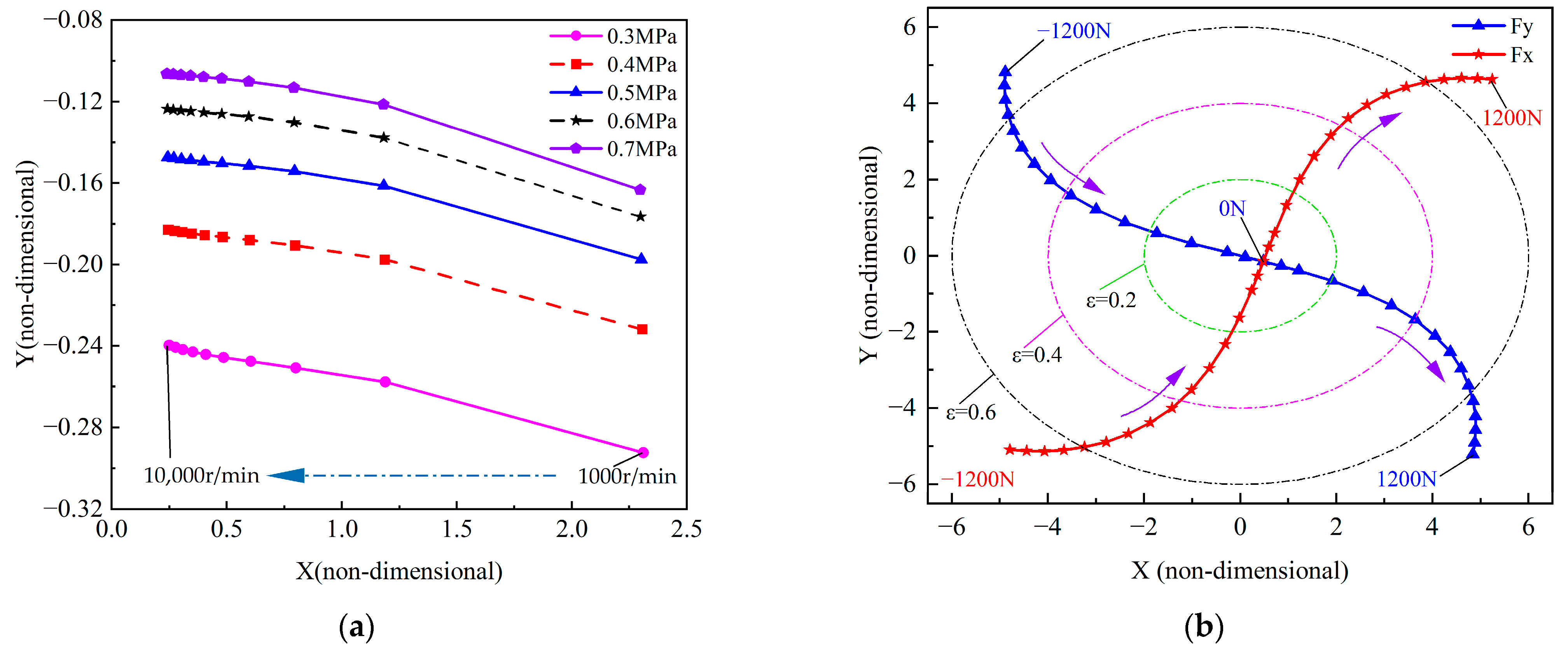
When the direction of external load on the rotor is unchanged and the amplitude continues to increase, the eccentricity increases nonlinearly. The equilibrium position initially moves away from the direction of the load and later moves closer to it. The main stiffness of the bearing increases with the increase in the external load, independent of the direction of the external load. When the horizontal external load increases gradually, the absolute value of the cross stiffness Kyx decreases, while the Kxy increases. Conversely, when the vertical external load gradually increases, the absolute value of the cross stiffness Kyx increases, while the Kxy decreases.
(3)
Without external load, the change in the equilibrium position and its stiffness with rotational speed and supply pressure is consistent with the conclusions of the references. And the reliability of the BIM is proved by the comparative analysis of the experiment and calculation, and the maximum error between them is 15.4%.

Author Contributions

Conceptualization, Y.H. and W.W.; methodology, H.Y. and S.Z.; software, G.Z. and Y.H.; validation, H.Y. and W.W.; formal analysis, S.L. and Y.L.; investigation, S.Z. and Y.L.; data curation, Y.H. and X.K.; writing—original draft preparation, Y.H. and X.K.; writing—review and editing, H.Y. and W.W.; visualization, S.L. and G.Z.; funding acquisition, H.Y. and S.L. All authors have read and agreed to the published version of the manuscript.

Funding

This research was funded by the National Nature Science Foundation of China, grant number 51875586; the Key Research Project of Higher Education Institutions in Henan Province, grant number 24A460030.

Data Availability Statement

Data are contained within the article.

Conflicts of Interest

The authors declare no conflicts of interest.

References

  1. Gao, Q.; Chen, W.; Lu, L.; Huo, D.; Cheng, K. Aerostatic bearings design and analysis with the application to precision engineering: State-of-the-art and future perspectives. Tribol. Int. 2019, 135, 1–17. [Google Scholar] [CrossRef]
  2. Hwang, J.; Park, C.H.; Kim, S.W. Estimation method for errors of an aerostatic planar XY stage based on measured profiles errors. Int. J. Adv. Manuf. Technol. 2010, 46, 877–883. [Google Scholar] [CrossRef]
  3. Abele, E.; Altintas, Y.; Brecher, C. Machine tool spindle units. CIRP Ann. 2010, 59, 781–802. [Google Scholar] [CrossRef]
  4. Tsai, M.H.; Hsu, T.Y.; Pai, K.R.; Shih, M.C. Precision position control of pneumatic servo table embedded with aerostatic bearing. J. Syst. Des. Dyn. 2008, 2, 940–949. [Google Scholar] [CrossRef]
  5. Pandey, N.P.; Tiwari, A. CFD Simulation of Air Bearing Material. Int. J. Sci. Res. Dev. 2010, 3, 126–129. [Google Scholar]
  6. Vainio, V.; Miettinen, M.; Majuri, J.; Theska, R.; Viitala, R. Manufacturing and static performance of porous aerostatic bearings. Precis. Eng. 2023, 84, 177–190. [Google Scholar] [CrossRef]
  7. Cui, W.; Li, S.; Zhu, B.; Yang, F.; Chen, B. Research on the influence of a micro-groove-orifice structure and its layout form on the static characteristics of aerostatic journal bearings under a high gas supply pressure. Adv. Mech. Eng. 2023, 15, 16878132231153263. [Google Scholar] [CrossRef]
  8. Zhang, J.; Deng, Z.; Zhang, K.; Jin, H.; Yuan, T.; Chen, C.; Su, Z.; Cao, Y.; Xie, Z.; Wu, D.; et al. The Influences of Different Parameters on the Static and Dynamic Performances of the Aerostatic Bearing. Lubricants 2023, 11, 130. [Google Scholar] [CrossRef]
  9. Ene, N.M.; Dimofte, F.; Keith, T.G. A stability analysis for a hydrodynamic three-wave journal bearing. Tribol. Int. 2008, 41, 434–442. [Google Scholar] [CrossRef]
  10. Li, Y.; Yu, M.; Ao, L.; Yue, Z. Thermohydrodynamic lubrication analysis on equilibrium position and dynamic coefficient of journal bearing. Trans. Nanjing Univ. Aeronaut. Astronaut. 2012, 29, 227–236. [Google Scholar] [CrossRef]
  11. Chakraborty, M.B.; Charraborti, D.P. Design and Development of Different Applications of PATB (Porous Aerostatic Thrust Bearing): A Review. Tribol.—Finn. J. Tribol. 2023, 40, 18–28. [Google Scholar] [CrossRef]
  12. Shuai, Q.; Wu, L.; Chen, Z. Solution of the three lobe’s journal center orbit under steady-state force. Mech. Eng. Autom. 2006, 2, 119–121. [Google Scholar]
  13. Qian, K.; Li, X. Lubrication simulation of three lobe journal bearing and solution for the equilibrium position problem. Lubr. Eng. 2008, 10, 52–54. [Google Scholar] [CrossRef]
  14. Wang, W.; Song, P.; Yu, H.; Zhang, G. Research on vibration amplitude of ultra-precision aerostatic motorized spindle under the combined action of rotor unbalance and hydrodynamic effect. Sensors 2023, 23, 496. [Google Scholar] [CrossRef] [PubMed]
  15. Yu, S.; Chen, S. Calculation of steady-state equilibrium position of tilting pad journal bearing in motorized spindle. China Mech. Eng. 2012, 23, 2492. [Google Scholar] [CrossRef]
  16. Wan, Z.; Wang, W.; Long, X.; Meng, G. On the calculation of journal static equilibrium position of oil film bearings. Lubr. Eng. 2019, 44, 11–16. [Google Scholar] [CrossRef]
  17. Zheng, T.; Hasebe, N. Calculation of equilibrium position and dynamic coefficients of a journal bearing using free boundary theory. J. Tribol. 2000, 122, 616–621. [Google Scholar] [CrossRef]
  18. Pokorný, J. An efficient method for establishing the static equilibrium position of the hydrodynamic tilting-pad journal bearings. Tribol. Int. 2021, 153, 106641. [Google Scholar] [CrossRef]
  19. Yang, M.; Xu, C. Twofold secant method of solving nonlinear equation. J. Henan Norm. Univ. 2010, 38, 14–16. [Google Scholar] [CrossRef]
  20. Zhou, W.; Wei, X.; Wang, L.; Wu, G. A super-linear iteration method for calculation of finite length journal bearing’s static equilibrium position. R. Soc. Open Sci. 2017, 4, 161059. [Google Scholar] [CrossRef]
  21. Deng, Z.; Cheng, W.; Cao, G. Solution of quiescent point in gas foil bearings. Bearing 2021, 9, 20–28. [Google Scholar] [CrossRef]
  22. Wen, B.; Gu, J.; Xia, S. Advanced Rotor Dynamics: Theory, Technology and Application; China Machine Press: Beijing, China, 1999; pp. 86–87. [Google Scholar]
  23. Jia, C.; Pang, H.; Ma, W.; Qiu, M. Analysis of dynamic characteristics and stability prediction of gas bearings. Ind. Lubr. Tribol. 2017, 69, 123–130. [Google Scholar] [CrossRef]
  24. Yang, L.; Li, H.; Yu, L. Dynamic stiffness and damping coefficients of aerodynamic tilting-pad journal bearings. Tribol. Int. 2007, 40, 1399–1410. [Google Scholar] [CrossRef]
  25. Wang, D.; Zhu, J. A finite element method for computing dynamic coefficient of hydrodynamic journal bearing. J. Aerosp. Power 1995, 69–71, 110. [Google Scholar] [CrossRef]
  26. Meng, S. Research on the rotary accuracy of the hydrostatic-dynamic spindle affected by journal geometric error and electromagnetic eccentricity. Ph.D. Thesis, Hunan University, Changsha, China, 2016. [Google Scholar]
  27. Qi, S.; Geng, H.; Lu, L. Dynamic Stiffness and Dynamic Damping Coefficients of Aerodynamic Bearings. J. Mech. Eng. 2007, 5, 91–98. [Google Scholar] [CrossRef]
  28. Li, Y.; Ao, L.; Li, L.; Yue, Z. Dynamic analysis method of dynamic character coefficient of hydrodynamic journal bearing. J. Mech. Eng. 2010, 46, 48–53. [Google Scholar] [CrossRef]
  29. Lo, C.; Wang, C.; Lee, Y. Performance analysis of high-speed spindle aerostatic bearings. Tribol. Int. 2005, 38, 5–14. [Google Scholar] [CrossRef]
Figure 1. Structure model of orifice throttling aerostatic bearing.
Lubricants 12 00085 g001
Figure 2. The influence of single direction displacement changes on bearing capacity. (a) Initial position. (b) Position after moving horizontally by +∆x.
Lubricants 12 00085 g002
Figure 4. Principle diagram of the BIM.
Lubricants 12 00085 g004
Figure 5. Flowchart for solving equilibrium positions using the BIM.
Lubricants 12 00085 g005
Figure 6. Comparison of convergence process of different methods.
Lubricants 12 00085 g006
Figure 7. (a) Equilibrium position under different pressures and rotating speeds. (b) Equilibrium position under different external loads.
Lubricants 12 00085 g007
Figure 8. (a) The influence of rotational speed on the stiffness at the equilibrium position. (b) The influence of supply pressure on the stiffness at the equilibrium position.
Lubricants 12 00085 g008
Figure 9. Stiffness changes at the equilibrium position under external load. (a) Horizontal load F x . (b) Vertical load F y .
Lubricants 12 00085 g009
Figure 10. Equilibrium position measurement experimental platform. (a) Schematic diagram. (b) Physical diagram. (1) air compressor, (2) air tank, (3) filter, (4) globe value, (5) solenoid throttle value, (6) flowmeter, (7) pressure gauge, (8) air inlet, (9) inductive probe, (10) motorized spindle, (11) digital display unit, (12) marble platform.
Lubricants 12 00085 g010
Figure 11. Experimental data and calculated data under different supply pressures.
Lubricants 12 00085 g011
Table 1. Bearing structure parameters and environmental parameters.
ParameterValue
Journal length L1 (mm)160
Journal radius R2 (mm)25
Mean air film thickness c (μm)10
Diameter of orifice d (mm)0.2
Row number of Orifice on journal bearing2
Orifice number of each row8
Rotor quality M (kg)6.5
Density of air ρ (kg·m−3)1.204
Supply pressure Ps (MPa)0.5
Environment pressure P (MPa)0.1
Viscosity of air μ (N·s·m−2)1.8 × 10⁻⁵
Table 2. Comparison of calculation results. (‘▲’ represents the calculation baseline for relative error).
Solution MethodCondition of ConvergenceIteration StepEquilibrium PositionRelative Error
Secant method1 × 10−222X = 0.17369\
Y = −0.20219\
Search method5 × 10−215X = 0.17342\
Y = −0.20228\
BIM1 × 10−34X = 0.173640.03%0.15%
Y = −0.202150.02%0.06%
Table 3. Mean air film thickness.
Journal Diameter
(mm)
Bearing Diameter
(mm)
Mean Air Film Thickness
(μm)
149.99750.02112
249.99850.02312.5
349.99650.02012
Average\\12.2
Disclaimer/Publisher’s Note: The statements, opinions and data contained in all publications are solely those of the individual author(s) and contributor(s) and not of MDPI and/or the editor(s). MDPI and/or the editor(s) disclaim responsibility for any injury to people or property resulting from any ideas, methods, instructions or products referred to in the content.

