An In-Depth Investigation of Faraday Depth Spectrum Using Synthetic Observations of Turbulent MHD Simulations

Abstract

In this paper, we present a detailed analysis of the Faraday depth (FD) spectrum and its clean components obtained through the application of the commonly used technique of Faraday rotation measure synthesis to analyze spectro-polarimetric data. To directly compare the Faraday depth spectrum with physical properties of a magneto-ionic medium, we generated synthetic broad-bandwidth spectro-polarimetric observations from magnetohydrodynamic (MHD) simulations of a transonic, isothermal, compressible turbulent medium. We find that correlated magnetic field structures give rise to a combination of spiky, localized peaks at certain FD values, and broad structures in the FD spectrum. Although most of these spiky FD structures appear narrow, giving an impression of a Faraday thin medium, we show that they arise from strong synchrotron emissivity at that FD. Strong emissivity at a FD can arise because of both strong spatially local polarized synchrotron emissivity at a FD or accumulation of weaker emissions along the distance through a medium that have Faraday depths within half the width of the rotation measure spread function. Such a complex Faraday depth spectrum is a natural consequence of MHD turbulence when the lines of sight pass through a few turbulent cells. This therefore complicates the convention of attributing narrow FD peaks to the presence of a Faraday-rotating medium along the line of sight. Our work shows that it is difficult to extract the FD along a line of sight from the Faraday depth spectrum using standard methods for a turbulent medium in which synchrotron emission and Faraday rotation occur simultaneously.

1. Introduction

The advent of broad-band receivers on all major radio telescopes in the last decade have opened up new avenues for investigating the properties of synchrotron-emitting relativistic plasma in astrophysical objects. Previously, one had to observe the same source at multiple, widely spaced frequencies to understand its polarization behavior. Broad-band radio spectro-polarimetric measurements of the Stokes Q and U parameters makes it possible to measure the variation of the polarized synchrotron emission over a wide contiguous frequency range which can provide crucial insights into the properties of the magneto-ionic medium for many sources in a much-reduced amount of observing time. Broad-band spectro-polarimetry has played a crucial role in unveiling the properties of magnetic fields in nearby galaxies [1,2,3], in high redshift galaxies [4,5], in active galactic nuclei (AGN; [6,7,8]) and the intergalactic medium [9]. In order to physically interpret such data, the technique of Faraday rotation measure (RM) synthesis [10,11] and direct fitting of the Stokes Q and U spectra of a polarized source with models of the magneto-ionic media, known as Stokes $Q,U$ fitting [6,12,13] have been developed. It is often not straightforward to interpret the results from these techniques and connect them to the physical properties of the magnetized plasmas being investigated [14].

Currently, several large-scale spectro-polarimetric campaigns are underway, mostly in the 1 to 5 GHz frequency range. On one hand, dedicated surveys with interferometers are being conducted to study the broad-band polarization properties of millions of extragalactic sources. For example, the Karl G. Jansky Very Large Array Sky Survey (VLASS; [15,16]), the Polarization Sky Survey of the Universe’s Magnetism (POSSUM; [17]), the QU Observations at Cm wavelength with Km baselines using ATCA1 (QUOCKA), the MeerKAT International GHz Tiered Extragalactic Exploration (MIGHTEE) Survey [18], and the recent LOFAR Two-meter Sky Survey (LoTSS; [19,20]) and S-PASS/ATCA [21]. Many more broad-band polarization surveys are planned in the future with the upcoming Square Kilometre Array (SKA).

On the other hand, to study the diffuse Galactic magneto-ionic medium, broad-band, large sky-area surveys below ∼15 GHz with single-dish telescopes have been undertaken, e.g., the Global Magneto-Ionic Medium Survey (GMIMS; [22]), the GALFA Continuum Transit Survey (GALFACTS; [23]), the S-band Polarization All Sky Survey (S-PASS; [24]), survey with the SKA-MPG prototype telescope [25], the C-Band All Sky Survey (C-BASS; [26]) and the Q-U-I JOint TEnerife (QUIJOTE; [27,28]).

With these broad-band polarization surveys, pressing astrophysical problems, such as black hole accretion and its connection to AGN jet launching mechanism, cosmic evolution of magnetic fields in galaxies, structure and strength of magnetic fields in the interstellar, intra-cluster and intergalactic medium will be investigated (see e.g., [29]). In addition to addressing astrophysical questions, these surveys will also contribute to the solution of fundamental cosmological questions via sensitive measurements of the Galactic diffuse synchrotron emission. This emission contaminates cosmological signals from the early Universe, such as the cosmic microwave background radiation, the cosmic dawn and the epoch of reionization.

Quantities related to the plasma properties of a magneto-ionic medium that can be derived from observations are: the intrinsic fractional polarization and angle of the linearly polarized synchrotron emission, the Faraday depth (FD) and its dispersion. The intrinsic fractional polarization is determined by the ratio of turbulent to ordered magnetic field strengths in the plane of the sky averaged over the telescope beam [30]. The intrinsic angle of the linearly polarized emission gives us information about the orientation of the ordered magnetic fields in the plane of the sky. The Faraday depth gives us information on the strength and direction of the average magnetic field parallel to the line of sight and its spatial variation can help us to distinguish between coherent and anisotropic random magnetic fields [31]. The dispersion of FD depends upon the properties of turbulent magnetic fields parallel to the line of sight. Hence, robust measurements of these quantities can provide insights into the 3-dimensional properties of magneto-ionic media in astrophysical sources. To measure them, RM synthesis and Stokes $Q,U$ fitting techniques are applied to broad-band spectro-polarimetric observations. Therefore, it is imperative to investigate, in detail, the scope of application of these data analysis techniques and their limitations. Understanding the efficacy and efficiency of these tools are of paramount importance for the success of the above mentioned surveys.

In this paper, we will focus on the technique of RM synthesis when it is applied to infer properties of diffuse medium, e.g., the Galactic interstellar medium (ISM). Starting with magnetohydrodynamic (MHD) simulations of isothermal, transonic, compressible turbulent plasma, similar to that observed in the Galactic ISM [32,33], we use raytracing to simulate broad-band spectro-polarimetric observations. Then, we apply RM synthesis to test what we can learn about the medium. The major questions we will investigate are: (1) Is there a difference in the nature of the Faraday depth spectrum obtained by applying RM synthesis to a medium with a realistic model of turbulence from MHD simulations versus the commonly used model of turbulence as a Gaussian random field? (2) What is the origin of complexity in the Faraday depth spectrum? (3) Can RM synthesis recover the Faraday depth of a diffuse medium which is simultaneously Faraday-rotating and emitting polarized synchrotron radiation?

This paper is organized as follows. In Section 2 we discuss in brief the techniques of RM synthesis and Stokes $Q,U$ fitting. We present in brief the salient features of the software package, COSMIC, for generating synthetic broad-band spectro-polarimetric data from MHD simulations in Section 3. In Section 4 we test the numerical performance of COSMIC using simulated media for which the broad-band polarization behavior is known analytically. We present details of the MHD simulations in Section 5 and synthetic polarization observations performed by applying COSMIC to the simulations are discussed in Section 6. In Section 7 we present a detailed analysis of the results obtained from RM synthesis and compare them to the intrinsic properties of the medium, and we summarize our findings in Section 8.

2. Common Spectro-Polarimetric Data Analysis Techniques

RM synthesis and Stokes $Q,U$ fitting are two commonly used techniques that are used to extract information from broad-band observations of polarized emission. The parameters of interest are the intrinsic fractional polarization ($p_{\mathrm{int}}$), intrinsic orientation of the polarization angle (${\theta }_0$), Faraday depth (FD) and the intrinsic dispersion of FD (${\sigma }_{\mathrm{FD}}$). In order to gain physical insights into an astrophysical system, robust measurement of these quantities are essential.

● Stokes parameter ($Q,U$) fitting: The technique of Stokes $Q,U$ fitting is a parametric fitting of the Stokes Q and U parameters’ wavelength ($\lambda$) dependent variation using models of a turbulent magneto-ionic media analytically derived, for example, in Burn [10], Tribble [34], Sokoloff et al. [30] and Rossetti et al. [35], and therefore requires assumptions on the nature of the medium being investigated. In Stokes $Q,U$ fitting, $p_{\mathrm{int}}$, ${\theta }_0$, FD and ${\sigma }_{\mathrm{FD}}$ are directly fitted for as model parameters. However, fitting is limited to a set of source models that might oversimplify the physics inside real radio sources and their environments. Moreover, often the broad-band Stokes Q and U data cannot be fitted by a single model and therefore linear combinations of models are used. Since increasing the number of models improves the quality of the fit by increasing the number of free parameters (principle of parsimony; [36]), statistical measures, such as the Bayesian inference criterion and/or Akaike information criterion are used to limit the number of models or to choose between degenerate fits [6,37]. However, Stokes $Q,U$ fitting has the advantage of also fitting for the spectral index of the polarized flux density (see [37]), which is not possible in RM synthesis and is one of the origins of complexity in the Faraday depth spectrum (e.g., [21,37]).

● Rotation measure synthesis: RM synthesis is a Fourier transform-like operation in which it is assumed that the linearly polarized radio source can be described as a sum of emitters at their respective Faraday depths, and is the Fourier transform of the frequency spectrum of the complex polarization2 [10,11]. Therefore, RM synthesis makes only a weak assumption about the physical properties of the magneto-ionic medium and is a non-parametric approach. Like any Fourier transform performed over a finite space (in this case a finite frequency coverage), the Faraday depth spectrum (variation of fractional polarization p or polarized intensity $PI$ as a function of FD) obtained from RM synthesis is convolved with a complicated response function determined by the frequency coverage of the observations. The response function is known as the rotation measure spread function (RMSF) and has sidelobes due to sharp cut-offs and gaps in the frequency coverage. Artefacts produced by the RMSF sidelobes can be deconvolved by applying the technique of RM clean [38]. In the case when Faraday rotation originates at multiple Faraday depths or Faraday depth varies contiguously through a volume, RM clean models a source as discrete $\delta$-function emitters in Faraday depth space known as clean components. The full width at half-maximum (FWHM) of the RMSF is determined by the bandwidth in ${\lambda }^2$ of the observations and it determines how well the emitters can be resolved in the Faraday depth space. The channel width of observations determines the maximum observable FD and the highest frequency end determines the sensitivity to the largest scale structure in the Faraday depth space (see for details [11]). This means that the results depend heavily on the frequency coverage used, and interpreting the RM cleaned Faraday depth spectra or the clean components can be a challenging task.

Another challenge of RM synthesis is the way $p_{\mathrm{int}}$, ${\theta }_0$, FD and ${\sigma }_{\mathrm{FD}}$ are determined from the Faraday depth spectrum. This comes down to a matter of choice for an individual investigator. In order to extract information on the physical quantities of magneto-ionic media, attempts have recently been made to describe the Faraday depth spectrum using parametric functions. In such an approach, the Faraday depth spectrum is modelled as a $\delta$-function for a purely Faraday-rotating medium, as a top-hat function for a simultaneously Faraday-rotating and synchrotron-emitting medium containing regular magnetic fields and constant densities of thermal and relativistic electrons, and as super-Gaussian function for a medium which contains both turbulent and regular magnetic fields [14,39,40]. Recently, Van Eck [41] proposed a model-free description of mapping the Faraday depth spectrum to polarized emission as a function of distance. The parametric descriptions, for both Faraday depth spectra and Stokes $Q,U$ fitting, implicitly assume a Gaussian random distribution of the components of the turbulent magnetic field. In contrast, the turbulent magnetic field and free electron distribution in the diffuse ISM, the focus of this paper, are expected to have spatially correlated structures, and are often non-Gaussian [42,43,44,45,46]. Furthermore, observations of extragalactic sources and the diffuse Galactic emission have revealed that FD spectra often show complicated structures [14,47,48] referred to as Faraday complexity. A part of the complexity can be introduced by the spectral index of the polarized emission, and hence RM synthesis is typically performed on fractional polarized parameters. Dedicated efforts, both mathematical and computational, are required to incorporate information on spectral index and Faraday depolarization into RM synthesis.

Because of these caveats, it is necessary to investigate the results of RM synthesis using MHD turbulence simulations which provide a more realistic magnetic field and Faraday depth distribution that are not described by simple Gaussian statistics.

3. COSMIC: From Physical Quantities to Stokes Parameters and Faraday Rotation

We have developed an end-to-end, fully parallelized, Python-based software package—Computerized Observations of Simulated MHD Inferred Cubes (COSMIC)—to generate synthetic data cubes of Stokes parameters as a function of frequency for further analysis. RM synthesis and RM clean are performed by integrating the pyrmsynth package3 into COSMIC. The code requires 3-dimensional (3-D) spatial cubes of the three magnetic field components (in units of μG) and the distribution of neutral or ionized gas density (in units of cm⁻³) computed from MHD simulations as inputs, in a Cartesian coordinate system. Depending on the type of MHD simulations, other optional inputs can be provided, such as the 3-D spatial distributions of temperature and the number density or energy spectrum of cosmic ray electrons (CREs). The default coordinate system is chosen such that the line of sight (LOS) is along the z-axis and, x- and y-axes are in the plane of the sky. However, COSMIC allows the user to choose the LOS axis perpendicular to any of the six faces of the cube.

For MHD simulations which do not contain cosmic rays, to compute the total synchrotron emission and the Stokes Q and U parameters of the linearly polarized synchrotron emission, a user can choose from several options to determine the number density of CREs ($n_{\mathrm{CRE}}$) and their energy spectrum. Similarly, to compute the Faraday depth, the number density of free electrons ($n_{\mathrm{e}}$) is estimated by choosing a suitable ionization model depending on the type of the simulations and other ancillary data computed in the simulations, such as the gas temperature. Using these, COSMIC computes the 2-D distribution of the total synchrotron intensity and the Stokes Q and U parameters on the plane of the sky across a frequency range specified by the user. Details of how observables are computed numerically and the different user-specified options are presented in Appendix A.

4. Benchmarking COSMIC with Analytic Models of Magneto-Ionic Media

To test the accuracy of the numerical calculations performed by COSMIC, we first compared outputs from it with simple models of magneto-ionic media whose frequency-dependent polarization behavior have analytic solutions. We simulated two types of radio sources which are simultaneously synchrotron emitting and Faraday-rotating: (1) a uniform slab containing a regular magnetic field and constant densities of free electrons and CREs [10,30]; (2) a volume that contains both regular and turbulent magnetic fields in which the turbulent fields have a Gaussian random distribution, known as the internal Faraday dispersion (IFD) model [30].

4.1. Uniform Slab Model

A uniform slab, also commonly referred to as a ‘Burn slab’ after Burn [10], is a synchrotron-emitting medium in which the strengths of the three magnetic field components and the densities of CRE and thermal electrons are all spatially constant. We generated such a medium on a 512 × 512 × 512 pixel³ mesh and assumed the mesh points to be separated by 1 pc. Therefore, the physical volume of the simulated uniform medium is 512 × 512 × 512 pc³. The values of the physical quantities used to simulate a uniform slab are listed in

Table 1. Setup parameters used to generate synthetic observations to test COSMIC with uniform slab and internal Faraday dispersion (IFD) models.

Parameter	Uniform Slab	IFD
Regular field strengths	$\langle B_x\rangle$ = 4 μG, $\langle B_y\rangle$ = 7 μG, $\langle B_z\rangle$ = 5 μG
Random field strengths:
${\sigma }_x$ (μG)	0	10
${\sigma }_y$ (μG)	0	10
${\sigma }_z$ (μG)	0	10
$n_{\mathrm{e}}$ (cm−3)	0.05	0.05
Box size	512 × 512 × 512 pc3
Mesh size	1 × 1 × 1 pc3
Spectral index	α = −0.8
Spectral curvature	None
Frequency range	${\nu }_{\min }$ = 0.5 GHz, ${\nu }_{\max }$ = 6 GHz
Number of channels	$n_{\mathrm{chan}}=500$

. We have used CRE density such that the total synchrotron flux density of the medium is 10 Jy at 1 GHz (see Appendix A.1). We assumed a power-law energy spectrum of the CREs, so that the synchrotron emissions also follow a power-law frequency spectrum with spectral index α = − 0.8 ($I_{\nu }\propto {\nu }^{\alpha }$, where $I_{\nu }$ is the intensity at frequency $\nu$).

For such a medium, the complex fractional polarization varies with wavelength $\lambda$ as [10,30],

$$p\left(\lambda \right)=p_{\mathrm{int}}{\displaystyle \frac{sin\mathrm{FD}{\lambda }^2}{\mathrm{FD}{\lambda }^2}}{\mathrm{e}}^{2i\left({\theta }_0+\frac{1}{2}\mathrm{FD}{\lambda }^2\right)}.$$

(1)

Here, $p_{\mathrm{int}}$ is the intrinsic fractional polarization of the medium, after accounting for any frequency-independent beam depolarization of the synchrotron emission that might be present, for example due to unresolved turbulent magnetic fields. As there is no beam or random magnetic field in this model, $p_{\mathrm{int}}$ is the same as the maximum fractional polarization $p_{\max }$ given in Equation (A5). The expected values of $p_{\mathrm{int}}$, FD and ${\theta }_0$ are listed in

Table 2. Expected values of physical parameters for the setup parameters used in Table 1 and values obtained using COSMIC.

Parameter	Uniform Slab		IFD
	Expected	Obtained	Expected	Obtained
$p_{\mathrm{int}}$	0.73	0.73	0.176	0.174
FD (rad m−2)	103.94	103.94	103.94	103.63
${\sigma }_{\mathrm{FD}}$ (rad m−2)	0.0	0.0	9.20	9.18
${\theta }_0$ (°)	150.26	150.25	150.26	150.25

.

Spectra of the total and linearly polarized synchrotron flux densities, $I_{\mathrm{sync}}$ and $PI$, respectively, obtained from COSMIC for a single LOS through the domain are shown in the top-left panel in Figure 1. The top-right and bottom-left panels in Figure 1 show the fractional Stokes parameters, i.e., $PI/I_{\mathrm{sync}}$, and $Q/I_{\mathrm{sync}}$ and $U/I_{\mathrm{sync}}$, respectively, as a function of ${\lambda }^2$, computed from the data using Equations (A1), (A9), (A10) and (A11). The bottom-right panel show the variation of the polarization angle, ${\theta }_0$, with ${\lambda }^2$. The dashed lines in Figure 1 show the analytical function given by Equation (1). To check the robustness of our numerical calculations, the parameters of the analytical model, namely $p_{\mathrm{int}}$, FD and ${\theta }_0$, were calculated directly from the COSMIC output. Please note that the fractional polarization and the angle of polarization are given by the amplitude and phase of the complex polarization, and are dependent on the wavelength (e.g., Equation (1)). Therefore, $p_{\mathrm{int}}$ and ${\theta }_0$ can either be determined at $\lambda =0$, which is unphysical, or when FD and/or ${\sigma }_{\mathrm{FD}}$ are $0\mathrm{rad}{\mathrm{m}}^{-2}$. We therefore computed $p_{\mathrm{int}}$ and ${\theta }_0$ by setting FD in each pixel of the 3-D cube to zero and then performing the synthetic observations. In Table 2, we present the expected values of $p_{\mathrm{int}}$, FD and ${\theta }_0$, and compare them with those computed from the cubes. All the values are in excellent agreement with the theoretical values.

4.2. Internal Dispersion Model

The internal Faraday dispersion (IFD) model describes a medium that is simultaneously synchrotron-emitting and Faraday-rotating in the presence of both regular and random magnetic fields, wherein the random field is isotropic, has Gaussian statistics and is delta-correlated (i.e., there are no correlated structures in the field). In other words, the correlation length is same as the length of the mesh point separation. We generated a volume of the same dimension as in Section 4.1, but in this case, the magnetic field strengths of each component in each 1 pc³ pixel were drawn at random from a Gaussian distribution. The mean value of the Gaussian represents the regular field strength along the corresponding direction and the standard deviation is a measure of the strength of the turbulent fields. Values of the different parameters used to generate the IFD volume are listed in Table 1.

The complex fractional polarization in such a medium varies with $\lambda$ as [30],

$$p\left(\lambda \right)=p_{\mathrm{int}}{\mathrm{e}}^{2i{\theta }_0}\left({\displaystyle \frac{1-exp[-(2{\sigma }_{\mathrm{FD}}^2{\lambda }^4-2i\mathrm{FD}{\lambda }^2)]}{2{\sigma }_{\mathrm{FD}}^2{\lambda }^4-2i\mathrm{FD}{\lambda }^2}}\right).$$

(2)

Here, ${\sigma }_{\mathrm{FD}}$ is the intrinsic dispersion of FD and is given by [49],

$${\sigma }_{\mathrm{FD}}=0.812\langle n_{\mathrm{e}}\rangle {\sigma }_{\parallel }\sqrt{{\displaystyle \frac{l_{0}L}{f_{\mathrm{V}}}}},$$

(3)

where ${\sigma }_{\parallel }$ is the strength of turbulent magnetic fields along the line of sight, $l_0$ is the correlation length of the product $n_{\mathrm{e}}{\sigma }_{\parallel }$, $L=512$ pc is the path-length through the magneto-ionic medium, and $f_{\mathrm{V}}$ is the volume filling factor of $n_{\mathrm{e}}$. In this example, since $n_{\mathrm{e}}$ is constant, $f_{\mathrm{V}}=1$, and $l_0=1$ pc as the random field is delta-correlated.

The intrinsic fractional linear polarization ($p_{\mathrm{int}}$) of the synchrotron emission originating from superposition of regular and isotropic random magnetic fields, and constant number density of CREs, is given by [30],

$$p_{\mathrm{int}}=p_{\max }{\displaystyle \frac{{\langle B_{\perp }\rangle }^2}{{\langle B_{\perp }\rangle }^2+{\sigma }_x^2+{\sigma }_y^2}}.$$

(4)

For our choice of parameters in Table 1, $p_{\mathrm{int}}$, ${\theta }_0$, FD and ${\sigma }_{\mathrm{FD}}$ are theoretically expected to be 0.176, 150.26°, 103.94 rad m⁻² and 9.2 rad m⁻², respectively. In Table 2, we compare these values with those directly obtained from COSMIC output using the same method as described at the end of the previous section. The values agree well with each other. In Figure 2, we show the variation of polarization fraction with $\lambda$ computed from synthetic observations of the simulated volume and they agree well with the analytic function given in Equation (2).

We should point out that in this case, we determined the frequency spectra of the polarization parameters shown in Figure 2 by averaging over 50 × 50 pixels² in the I, Q and U images. This is done to ensure that there are a sufficient number of pixels to capture the Gaussian statistics generated by standard routines for generating random numbers in Python. For smaller averaging areas, significant deviations of the synthetic data from the analytic function is observed, especially towards longer wavelengths. A comparison of the variation of fractional polarization with ${\lambda }^2$ obtained from synthetic observations by averaging over different areas is shown in the inset of the top right-hand panel of Figure 2. At shorter wavelengths, all synthetic observations agree well with the analytic function.

5. Applying COSMIC to MHD Simulations of a Turbulent Medium

The magnetic fields and free electrons in the ISM have more complicated distributions than can be described by simple delta-correlated Gaussian statistics, for example they can have spatial correlations in their structure (see e.g., [1,44,46]). Therefore, investigating the broad-band properties of the linearly polarized synchrotron emission from realistic MHD simulations is required, especially with several on-going and upcoming polarization surveys of the Milky Way’s diffuse emission.

Here we apply COSMIC to MHD simulations of isothermal, compressible and transonic turbulence in the ISM from Burkhart et al. [43,50]. Polarization observations of the Galactic plane and Galactic Hi 21 cm observations of the warm gas have confirmed the transonic nature of turbulence in the ISM [32,33,51]. The simulation set up is similar to that of past works [43,52,53]. We refer to these works for the details of the numerical setup and we only provide a short overview here. The simulation used here is a 3-D turbulent box of isothermal compressible MHD turbulence with a resolution 512³, and each mesh point is separated by 1 pc. The code is a third-order accurate essentially nonoscillatory scheme which solves the ideal MHD equations in a periodic box with purely solenoidal driving of the flow at a scale 2.5 times smaller than the domain size, i.e., ∼200 pc. The simulation has two control parameters: the sonic Mach number ($M_{\mathrm{s}}=v/c_{\mathrm{s}}$, where v is the flow velocity and $c_{\mathrm{s}}$ is the sound speed) and Alfvénic Mach number ($M_{\mathrm{A}}=v/v_{\mathrm{A}}$, where $v_{\mathrm{A}}$ is the Alfvén speed). In these simulations, we used $M_{\mathrm{s}}\approx 2.0$ and $M_{\mathrm{A}}\approx 0.7$. The magnetic field consists of a regular background field ($B_{\mathrm{ext}}$) and a turbulent field (b), i.e., $B=B_{\mathrm{ext}}+b$ with the magnetic field initialized along a single preferred direction. In the choice of our coordinate system, the regular field is along the x-direction and has a strength of 10 μG. This regular field will not contribute to Faraday depth as the LOS is along the z-direction.

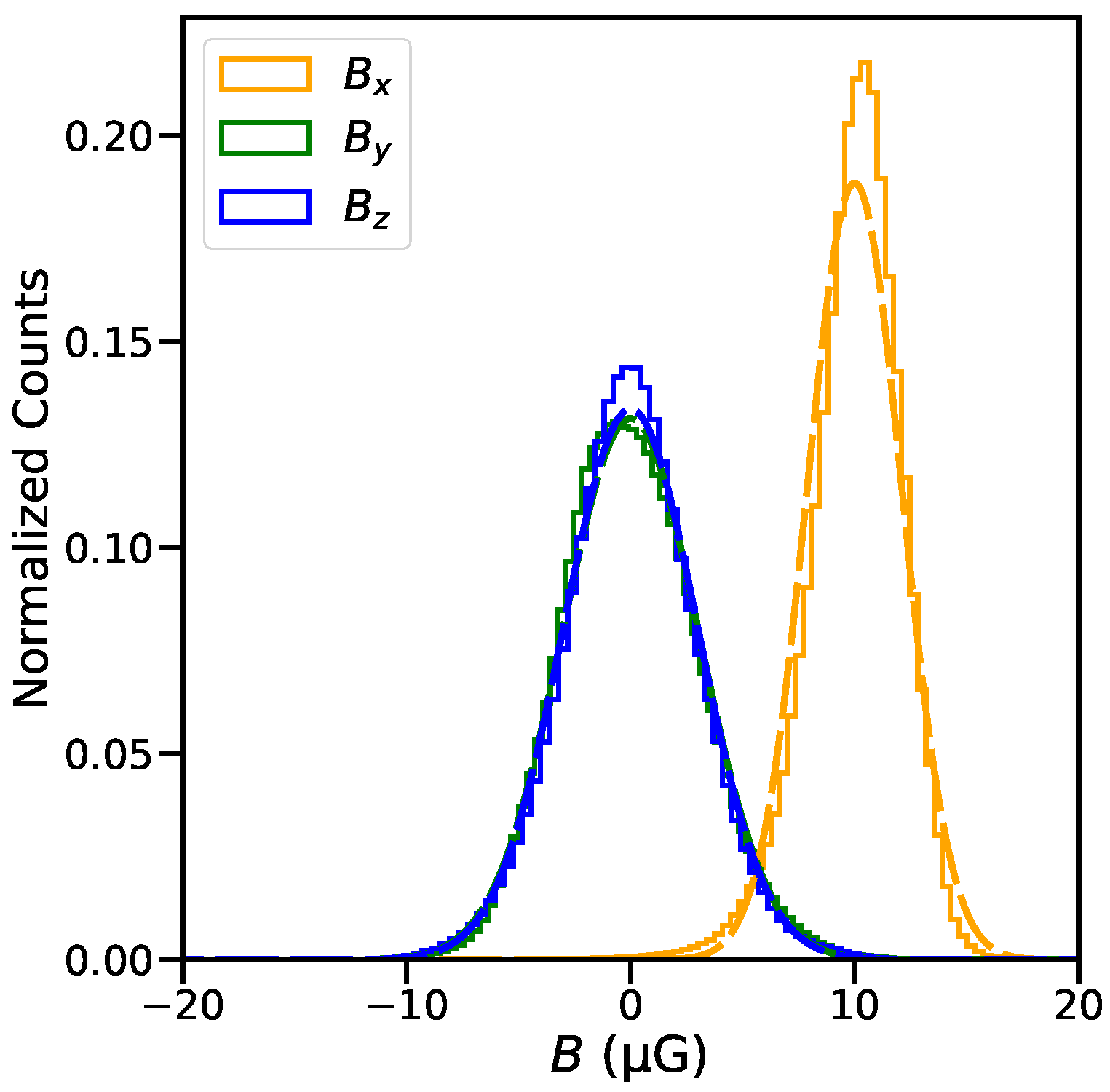
The distribution of the strengths of the three magnetic field components over the entire simulation volume is shown in Figure 3. The corresponding dashed lines are for equivalent Gaussian distributions computed from the mean and standard deviation of the corresponding field component. The distribution of $B_x$ shows deviation from a Gaussian distribution, while that for $B_y$ and $B_z$ agrees well with Gaussian distributions. We must stress, although the distributions of the magnetic field components closely resembles a Gaussian distribution, spatially they are correlated on the driving scale of turbulence in these simulations, unlike the delta-correlated Gaussian fields described in Section 4.2. For details regarding their structural and statistical properties we refer interested readers to Burkhart et al. [43,50]. To summarize, physical specifications of the simulations are as follows: (1) Physical size of the simulation volume is 512 × 512 × 512 pc³. (2) Mesh resolution of the simulation is 1 × 1 × 1 pc³. (3) The mean magnetic field strengths are: $\langle B_x\rangle$ = 10 μG and $\langle B_y\rangle =\langle B_z\rangle$ ≈ 0 μG; and the three components have dispersions ${\sigma }_x$ = 2 μG, ${\sigma }_y$ = 3 μG and ${\sigma }_z$ = 3 μG. Thus, the ratio of regular to turbulent field strengths in this simulation is $\sim 2$. We would like to emphasize that this regular field, local to the simulated volume, would only contribute to the polarized intensity of the synthetic observations, unlike those observed in external galaxies. Polarization measurements in external galaxies are performed with comparatively lower spatial resolution. Therefore, they are mostly sensitive to the ordered component of the magnetic field within the beam, or to the large-scale regular fields, and therefore in external galaxies the ordered fields are observed to be about three times weaker than the turbulent fields [54].

As the MHD simulation used in this work is isothermal and in thermal equilibrium, the ionization fraction, $f_{\mathrm{ion}}$, of neutral hydrogen is assumed to be constant throughout the volume and can be chosen to compute the free electron density $n_{\mathrm{e}}$ (see Appendix A.2). Increasing $f_{\mathrm{ion}}$ increases $n_{\mathrm{e}}$ and thereby the amount of Faraday rotation (${\mathrm{FD}}_{\mathrm{cell}}$) in each cell of the MHD cube, which increases the amount of Faraday depolarization through the entire LOS. 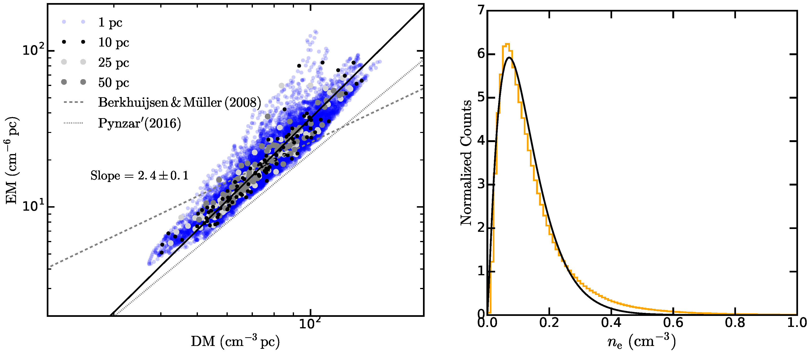To find physically motivated value for $f_{\mathrm{ion}}$, we produced maps of emission measure ($\mathrm{EM}=\int n_{\mathrm{e}}^2\mathrm{d}l$) and dispersion measure ($\mathrm{DM}=\int n_{\mathrm{e}}\mathrm{d}l$) for various values of $f_{\mathrm{ion}}$ and compared EM vs. DM by averaging over different areas [55]. In the left-hand panel of Figure 4 we show the variation of EM as a function of DM. The slope of the best-fit line (shown as the black line) is found to be $2.4\pm 0.1$ indicating that the simulation used here is strongly clumpy with low $f_{\mathrm{V}}$. We varied $f_{\mathrm{ion}}$ such that the amplitude roughly matches with observations of the Galactic ISM. For example, Berkhuijsen and Müller [56] found a slope of 1.15 for the EM vs. DM relation for the diffuse ionized gas around the Solar neighborhood with mean $f_{\mathrm{V}}=0.08$. In denser and clumpier ISM with $f_{\mathrm{V}}<0.06$, the slope of the EM vs. DM relation was estimated to be 2 by Pynzar’ [57].

For the simulations used here, the amplitude of the EM vs. DM relation agrees well with that observed in our Galaxy for $f_{\mathrm{ion}}=0.5$ (see Figure 4). In the right-hand panel of Figure 4, we show the distribution of $n_{\mathrm{e}}$ in the simulation volume for $f_{\mathrm{ion}}=0.5$. Here, the median $n_{\mathrm{e}}$ is $0.11{\mathrm{cm}}^{-3}$ and it has a maximum value of $3.5{\mathrm{cm}}^{-3}$. Such values of $n_{\mathrm{e}}$ are typically observed within Galactic latitudes $\pm {15}^{°}$ [57,58]. The distribution of $n_{\mathrm{e}}$ is well approximated by a Gamma distribution (solid black line) with shape parameter ≈2.25 and inverse scale parameter ≈0.06, i.e., an expectation value for $n_{\mathrm{e}}\approx 0.13{\mathrm{cm}}^{-3}$.

For the values of $n_{\mathrm{e}}$ and $B_{\parallel }$ in these MHD simulations, <0.3% of the $1{\mathrm{pc}}^3$ mesh points have $|{\mathrm{FD}}_{\mathrm{cell}}|>3\mathrm{rad}{\mathrm{m}}^{-2}$ and $<1\%$ mesh points have $|{\mathrm{FD}}_{\mathrm{cell}}|>2\mathrm{rad}{\mathrm{m}}^{-2}$. That means, within the cell, $<0.3\%$ and $<1\%$ of the mesh points undergo Faraday depolarization of $>20\%$ and $>10\%$, respectively, at frequencies below ∼0.5 GHz. Calculations of the polarization parameters in COSMIC assumes that the Faraday depolarization in a single mesh point is negligible (see Appendix A.2, Appendix A.3 and Appendix A.4). Therefore, for these simulations COSMIC can be safely applied to frequencies above 0.5 GHz.

The following options were used to compute the synthetic spectra of $I_{\mathrm{sync}}$, $PI$, Stokes Q and U in the rest of this paper. (1) As the simulations do not contain cosmic rays and the typical CRE propagation lengths are expected to be comparable to or larger than the size of the simulation box (see Appendix A.1), we assume that the CREs are uniformly distributed throughout the 3-D volume of the simulation. (2) The CREs follow a power-law energy spectra with the same energy index throughout the volume. Thus, the synchrotron intensity spectral index ($\alpha$) is constant, both spatially and with frequency, with $\alpha =-0.8$ defined as $I_{\mathrm{sync}}\propto {\nu }^{\alpha }$. (3) $n_{\mathrm{CRE}}$ is normalized such that the total synchrotron flux density at 1 GHz integrated over the entire volume is 10 Jy (see Appendix A.1). Note that the amplitude of the frequency spectrum of intrinsic emissivities of the total synchrotron emission, and Stokes Q and U parameters can be scaled depending on the unknown $n_{\mathrm{CRE}}$ without affecting the relative frequency variation. (4) The ionization fraction is constant throughout the volume with $f_{\mathrm{ion}}=0.5$.

In the following analyses, we have not added any systematic effects arising from combining data observed using multiple telescope receivers into one large bandwidth or telescope noise. Also, the synthetic observations are not sampled using $u-v$ coverage of an interferometer and therefore mimics observations performed using a single-dish radio telescope. This is because we want to investigate what can be learnt about a medium from RM synthesis under ideal conditions.

6. Synthetic Observations of MHD Simulations

We compute synthetic spectra of the total and linearly polarized quantities that describe the synchrotron emission of the volume in the frequency range 0.5 to 6 GHz divided into 500 frequency channels. The choice of lowest frequency is determined by the need to minimize Faraday depolarization within each 3-D mesh point (see Section 5) and the highest frequency is chosen such that the synthetic observations are sensitive to broad structures in the Faraday depth space and roughly corresponds to the high frequency end of on-going spectro-polarimetric surveys of the diffuse Galactic synchrotron emission (e.g., [26]).

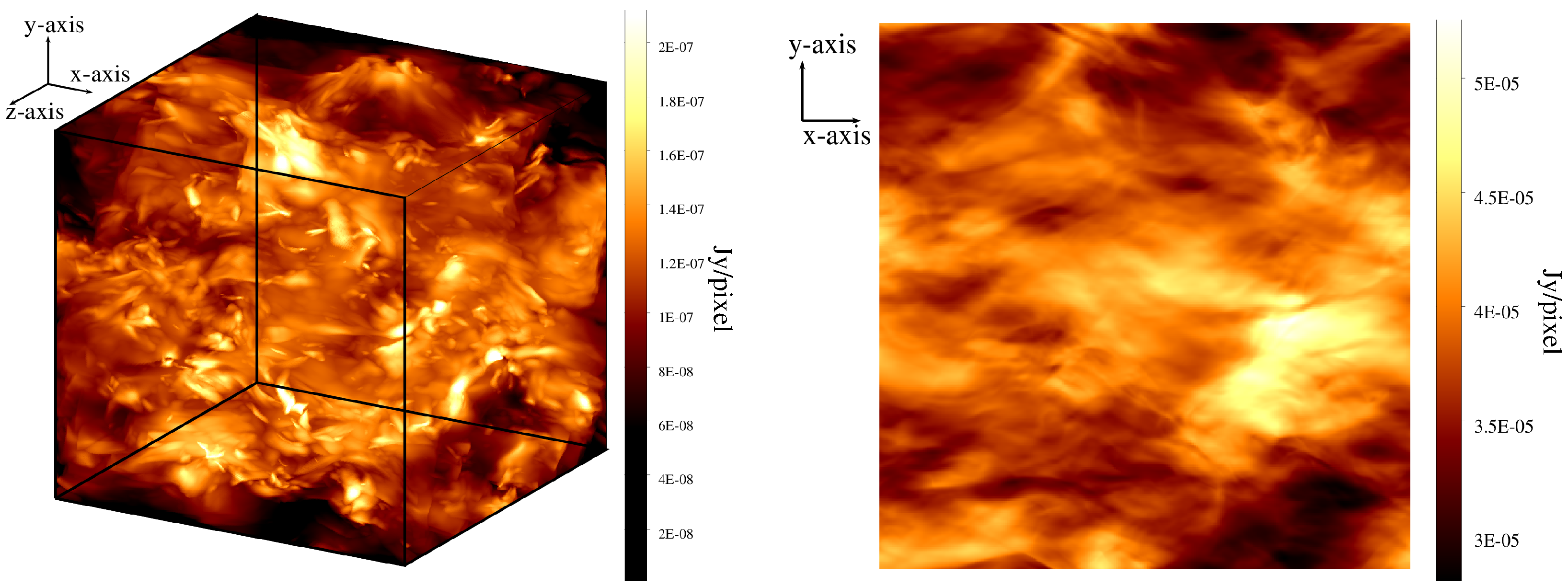
In the left-hand panel of Figure 5, we show the 3-D total synchrotron emissivity of the simulated volume at 1 GHz. The right-hand panel shows the projected 2-D map of the total synchrotron intensity ($I_{\mathrm{sync}}$) obtained by integrating the 3-D cube in the left-hand panel along the z-axis, our LOS axis. Since we have assumed a constant density of CREs, all the structure in this image arises due to the variations of synchrotron emissivity caused by fluctuations of the magnetic field component in the plane of the sky, both along and across the LOS.

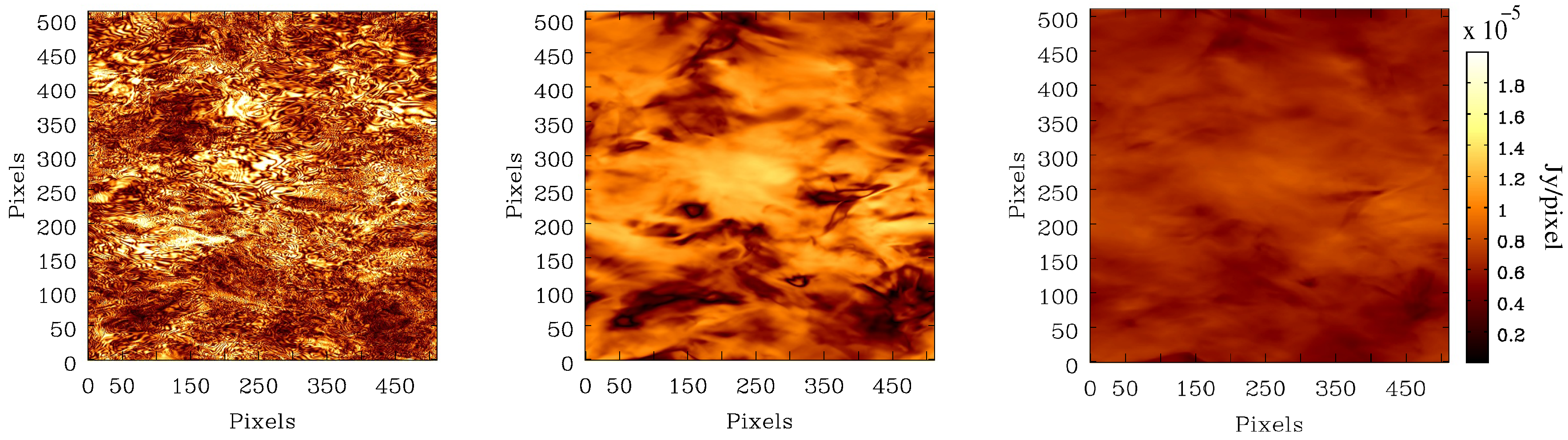
In Figure 6, we show the polarized intensities at 0.5, 1.5 and 5 GHz. Due to frequency-dependent Faraday depolarization, the polarized emission develops small-scale structures at lower frequencies. This is due to fluctuations in $B_{\parallel }$ along and across the lines of sight. For frequencies below ∼3 GHz, where most of the polarized surveys of Galactic diffuse emission have been performed (e.g., [48,59,60,61]), the polarized emission shows some ‘canal-like’ small-scale structures (e.g., [62]). Due to severe Faraday depolarization at 0.5 GHz, the polarized emission show structures on scales of a few pixels. The maps of Stokes Q and U parameters also show a similar trend in their structural properties with frequency. This underlines the challenge of combining interferometric observations of diffuse emission at different frequencies. The smooth, diffuse structure in Stokes Q and U at the highest frequencies will be filtered out from the data. This does not happen at lower frequencies because different sightlines undergo different amounts of Faraday depolarization, leading to rapid variations on small scales. This issue cannot be overcome even if frequency-scaled interferometer arrays are used to match the $u-v$ coverage at different frequencies.

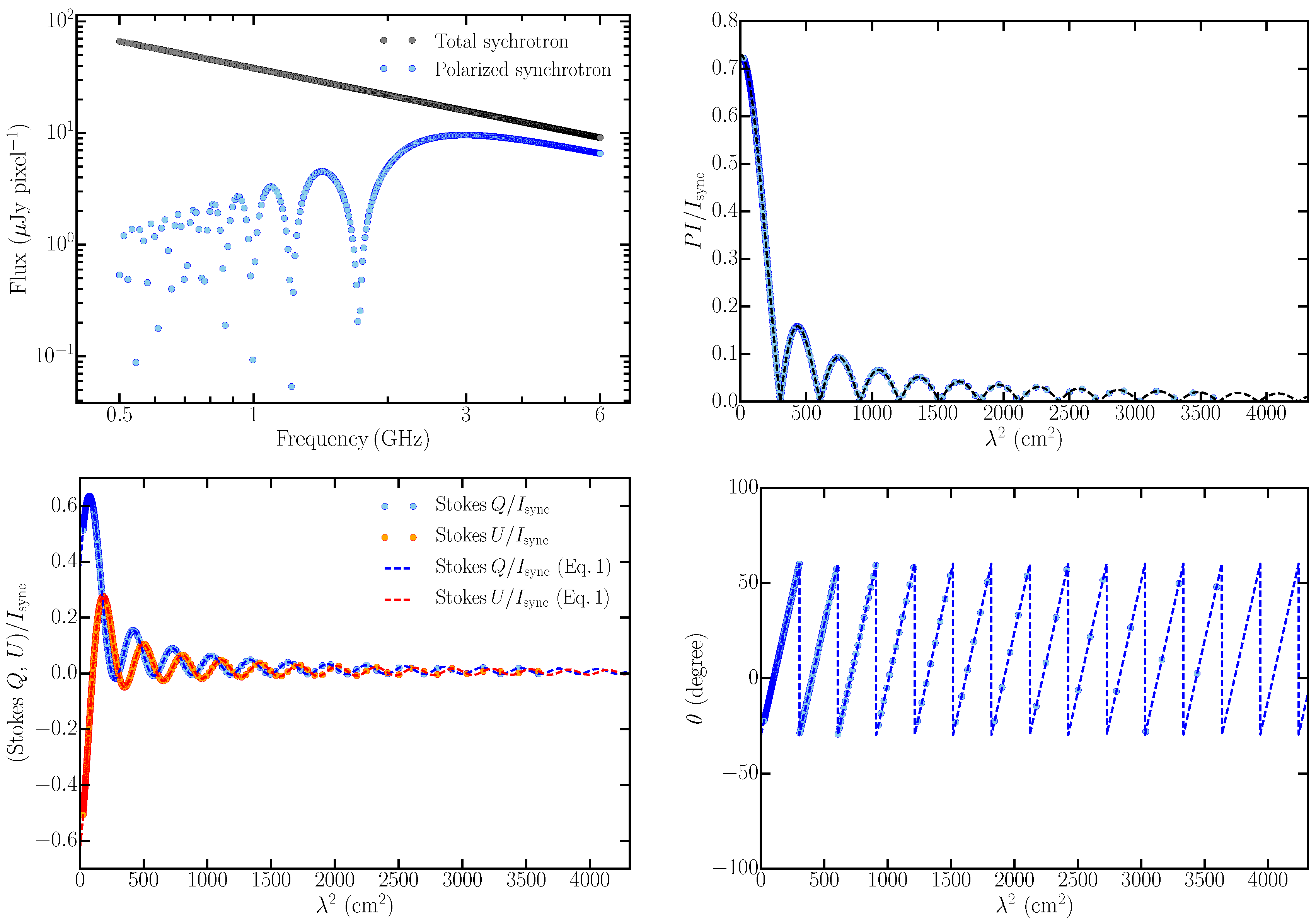
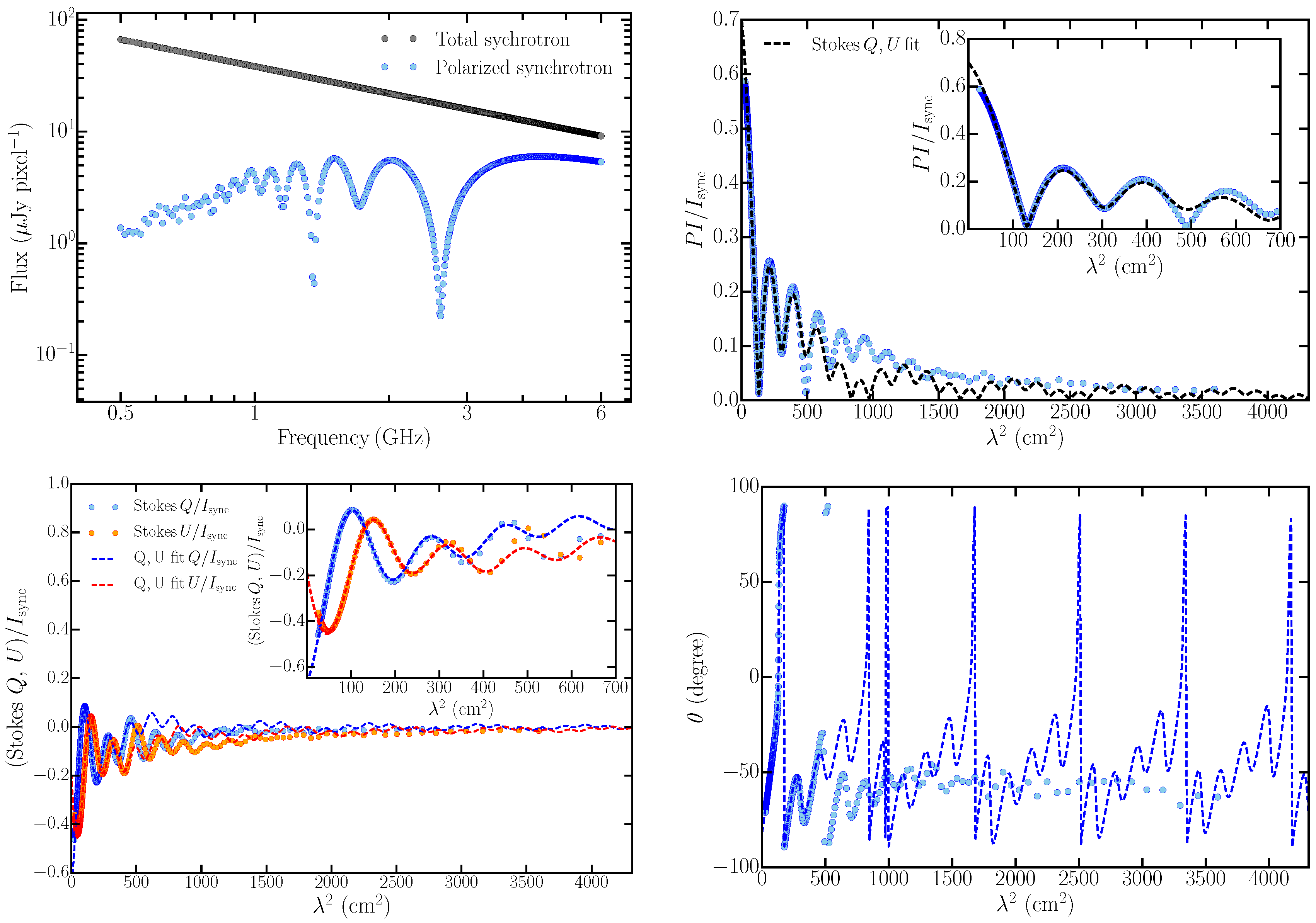
6.1. Broad-Band Spectra of Stokes Parameters

Figure 7 shows the synthetic spectra of the total synchrotron emission and parameters of linearly polarized synchrotron emission between 0.5 and 6 GHz. All the quantities are computed by averaging over a randomly chosen 30 × 30 pixel² region corresponding to a spatial scale of 30 × 30 pc². The polarized emission at lower frequencies (<1 GHz) show strong frequency-dependent variations. This implies that at low frequencies, the small-scale polarized structures seen in the left-hand panel of Figure 7 are also expected to vary strongly with slight changes in frequency.

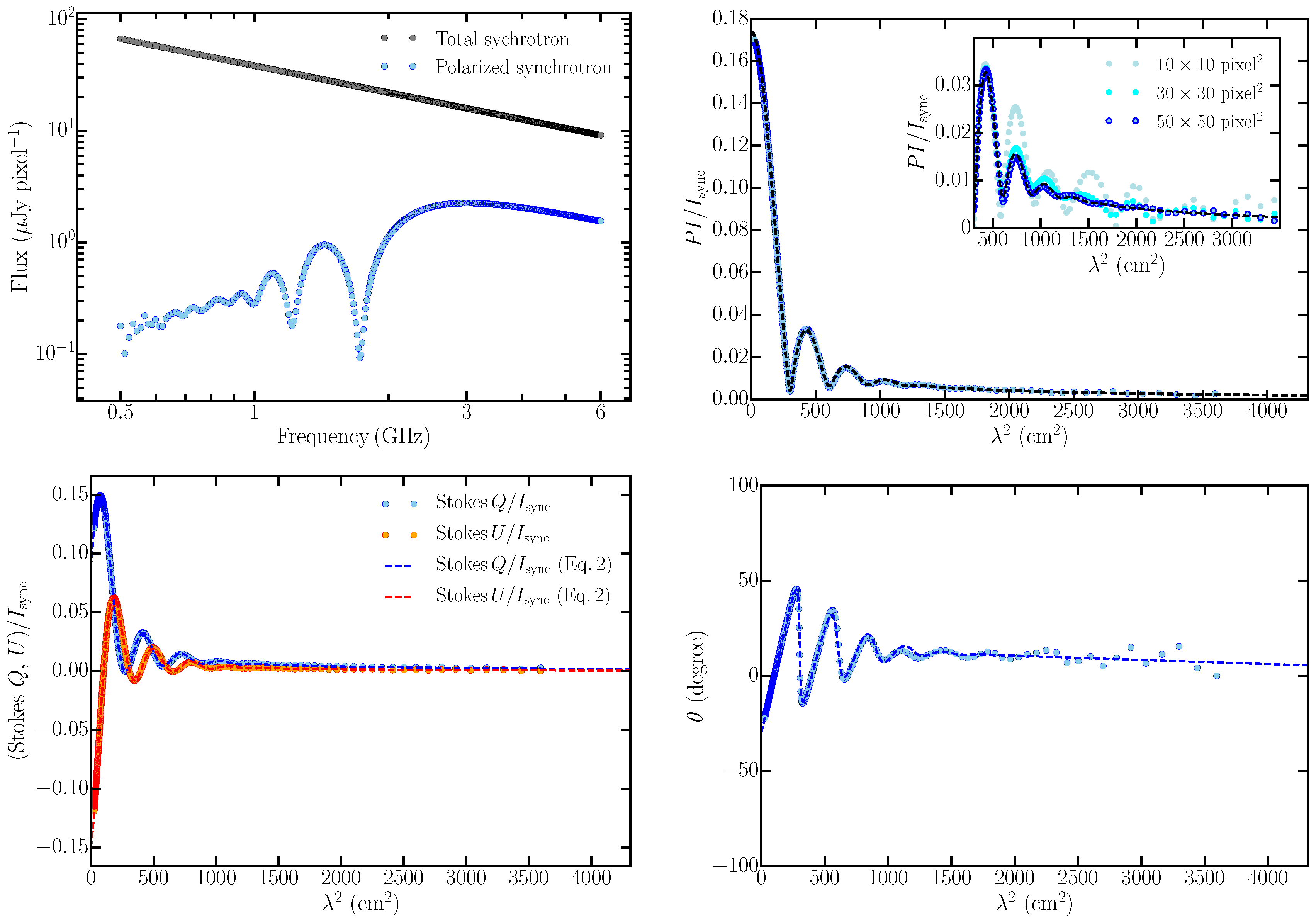
Although Stokes $Q,U$ fitting is not the main focus of this work, we nonetheless present in brief the result of fitting the synthetic data shown in Figure 7. Stokes $Q,U$ fitting was performed using analytical functions for several types of depolarization models described in Sokoloff et al. [30] and O’Sullivan et al. [7] and their linear combinations. In our Stokes $Q,U$ fitting routine, we allow combination of a maximum of three depolarization models and use the corrected Akaike information criteria [63,64] to choose the best-fit model. Because of the strong variation of the Stokes Q and U parameters in the longer wavelength regime (in this case roughly > 700 cm² corresponding to frequencies < 1.1 GHz), the combination of three depolarization models is not sufficient to fit the Stokes Q and U parameter spectra for the entire wavelength range considered here. However, for wavelengths below 700 cm², fits converged successfully (inset in Figure 7). For the synthetic data in Figure 7, the best-fit was obtained with a linear combination of three internal Faraday depolarization components (Equation (2)). In fact, none of the regions we have investigated in these simulations could be fitted by a single depolarization model, in contrast to the simulated volumes in Section 4. This implies that spatially correlated distributions of the magnetic fields and/or thermal electron densities, as in these MHD simulations, could possibly give rise to multiple polarized components (also see Section 7.2) that have different wavelength-dependent depolarization behaviors.

The failure of Stokes $Q,U$ fitting in being able to fit the synthetic data below ∼1 GHz with three or less components brings to light an important aspect about the technique. To our knowledge, most of the Stokes $Q,U$ fitting in the literature has been applied to data above ∼1 GHz, or to high redshift sources for which the rest-frame emission originated close to 1 GHz or higher, and up to three polarization components has been sufficient to fit those data. It will be interesting to investigate the performance of Stokes $Q,U$ fitting when broad-band spectro-polarimetric data is acquired below 1 GHz for many sources with future surveys. A detailed investigation of the results of Stokes $Q,U$ fitting, the generic properties of the method in connection to different types of MHD simulations and the optimum number of depolarization models required to extract maximum physical insights into a diffuse magneto-ionic medium is beyond the scope of this paper, and will be discussed elsewhere.

6.2. Reconstructed Faraday Depth Map

To construct the Faraday depth map from the synthetic Stokes Q and U parameters, we applied the technique of RM synthesis. In order to avoid complications arising from the effects of spectral index [21,37], all analysis pertaining to RM synthesis were performed on fractional polarization quantities, i.e., $q=Q/I_{\mathrm{sync}}$, $u=U/I_{\mathrm{sync}}$ and $p=PI/I_{\mathrm{sync}}$. For the frequency setup used here, the RMSF has a FWHM of 10 rad m⁻² and is sensitive to extended Faraday depth structures up to ∼1250 rad m⁻² (see [11]). This is sufficient to perform high Faraday depth resolution investigation of these synthetic observations without being affected by missing large-scale Faraday depth structures.

The Faraday depth spectrum was computed for the search range −3000 to +3000 rad m⁻² with a step size of 0.5 rad m⁻². Since we have not added any noise to the synthetic data, RM clean was performed by setting loop gain to 0.02 and with 1000 cleaning iterations. This allows cleaning down to the minimum fractional emissivity of the 3-D mesh points in the simulated volume. 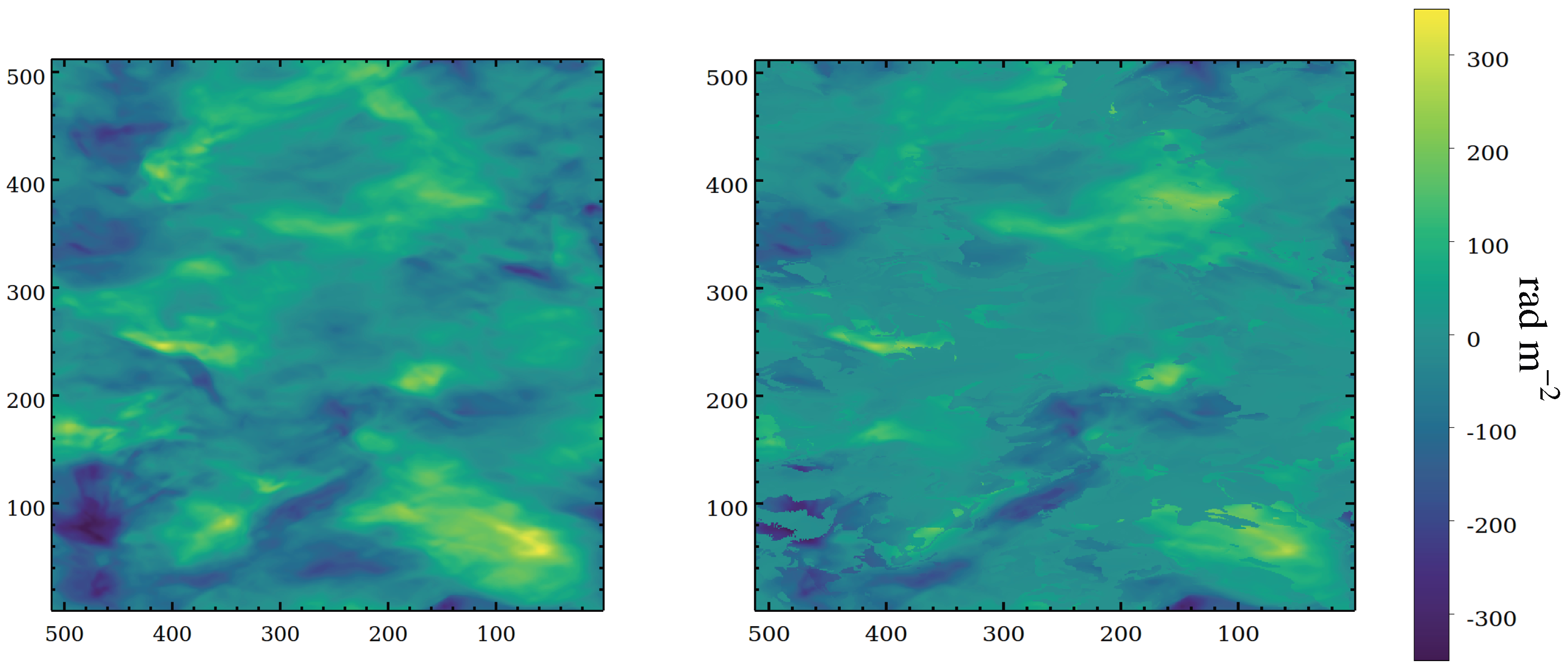Synthetic observations are processed using the pyrmsynth implementation of RM synthesis to produce a Faraday depth spectrum which is then deconvolved using RM clean. In Figure 8, we show the expected Faraday depth map from the MHD simulations (${\mathrm{FD}}_{\mathrm{MHD}}=0.812\int n_{\mathrm{e}}{B}_{\parallel }\mathrm{d}l$, computed using Equation (A4) on the left-hand side and the reconstructed Faraday depth map computed using RM synthesis (${\mathrm{FD}}_{\mathrm{RM}\mathrm{synthesis}}$) on the right-hand side. We have determined ${\mathrm{FD}}_{\mathrm{RM}\mathrm{synthesis}}$ in a pixel as the location of the peak of the Faraday depth spectrum computed by fitting a parabola. The spatial features in the reconstructed FD map broadly matches with the ${\mathrm{FD}}_{\mathrm{MHD}}$ map, but the magnitudes differ significantly. Also, some regions of the reconstructed FD map show sharp jumps across neighboring pixels. In the next section we will discuss in detail the complexity of determining the Faraday depth from the Faraday depth spectrum.

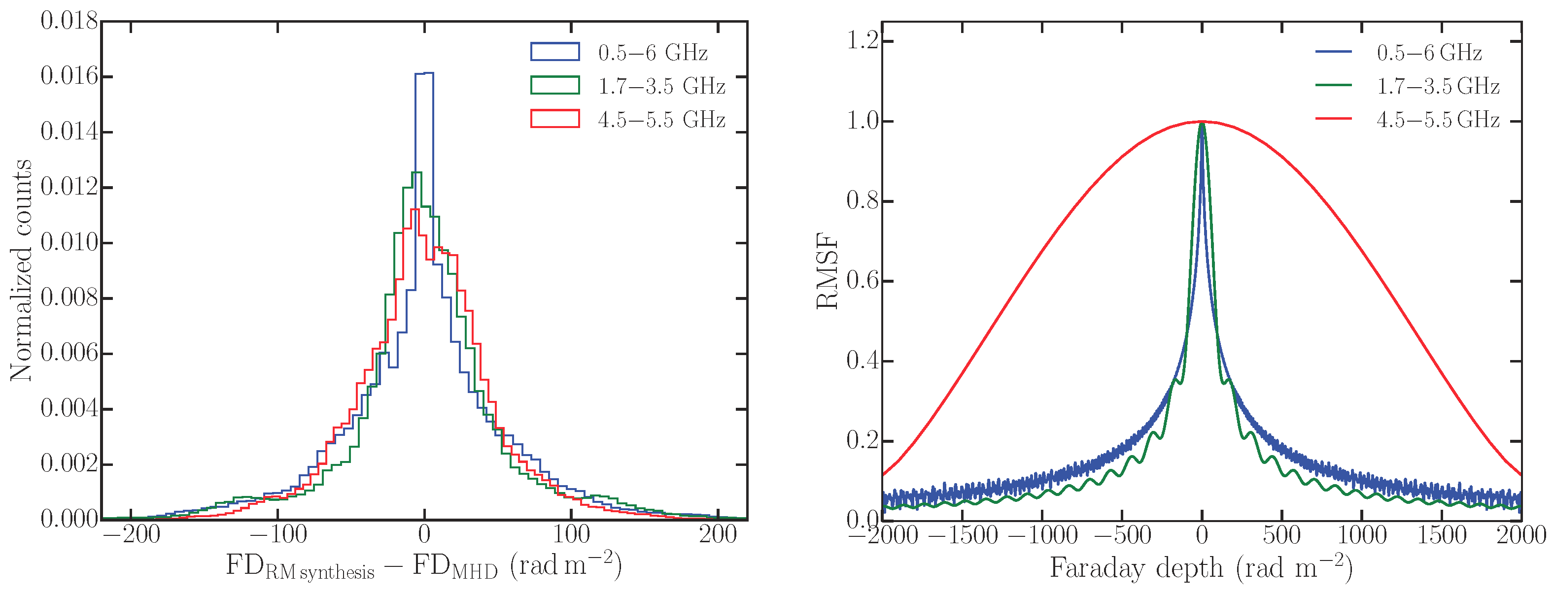
In the left-hand panel of Figure 9, we show the distribution of the difference ${\mathrm{FD}}_{\mathrm{RM}\mathrm{synthesis}}-{\mathrm{FD}}_{\mathrm{MHD}}$. The FWHM of the RMSF for the synthetic observations of only 10 rad m⁻², which in combination with the signal-to-noise ratio, gives an estimate of the error of determined FD. Since, we have not added any noise to the synthetic data, the estimated ${\mathrm{FD}}_{\mathrm{RM}\mathrm{synthesis}}$ is expected to have vanishing error. However, ${\mathrm{FD}}_{\mathrm{RM}\mathrm{synthesis}}$ is significantly off with respect to the expected ${\mathrm{FD}}_{\mathrm{MHD}}$ by up to ±200 rad m⁻². This is mainly because of the way FD is determined from Faraday depth spectra that are highly complex as discussed in the next section. To assess possible systematic effects arising from the RMSF and/or sensitivity to large Faraday depth structures, we also computed ${\mathrm{FD}}_{\mathrm{RM}\mathrm{synthesis}}$ for different frequency coverages. The different histograms in Figure 9 (left-hand panel) show the distribution of ${\mathrm{FD}}_{\mathrm{RM}\mathrm{synthesis}}-{\mathrm{FD}}_{\mathrm{MHD}}$ for the different frequency coverages. The respective RMSFs are shown in the right-hand panel of Figure 9. For none of the frequency ranges is FD recovered with sufficient accuracy.

7. Comparing Faraday Depth Spectrum Obtained by RM Synthesis with the Intrinsic Spectrum of a Turbulent Medium

In this section, we examine Faraday depth spectrum of individual lines of sight through both the simple benchmark data cubes of Section 4 and the MHD turbulence data cube described in Section 5, using two different methods. First, the COSMIC code is used to generate Stokes Q and U values using the observational setup described in Section 6 and Faraday depth spectra were computed in the same way described in Section 6.2. Second, we calculate the polarized emissivity and the local Faraday depth at each position along the same lines of sight to generate a model of the intrinsic Faraday depth spectrum for that LOS.

We wish to know how close the two Faraday depth spectra are for a realistic model of a turbulent, synchrotron-emitting medium. In particular, does a spectrum obtained by RM synthesis give a true representation of the emissivity distribution by Faraday depth that the medium actually produces? If the answer to this is no, then what is the connection between the Faraday depth spectrum and the physical state of the emitting region? While the answers to these questions will probably not be surprising, with hindsight, to someone familiar with the method, we will gain valuable insights into the nature of the problem from this investigation.

7.1. Faraday Depth Spectra of Analytical Models

We first illustrate the process using the two simple models for the distribution of emissivity and Faraday depth described in Section 4: a uniform slab and an internal Faraday dispersion volume with delta-correlated Gaussian random fields. Artefacts introduced by the RM synthesis and RM clean algorithms will be clearly visible, the data will provide a useful reference point for comparisons later, and we shall begin to see the difficulties in discriminating between very different sources using the technique.

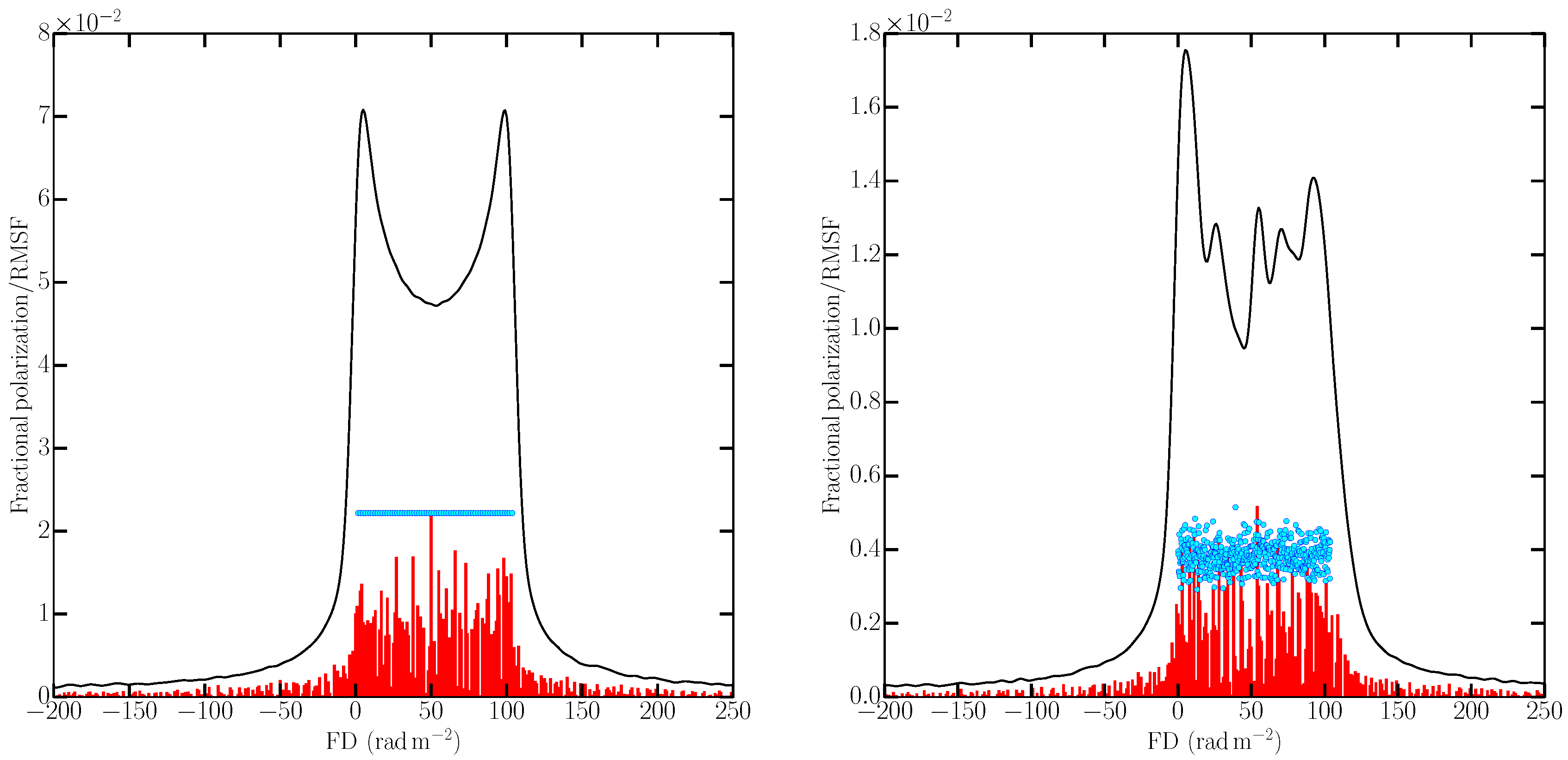
In Figure 10, for both the uniform slab and Gaussian random field models, we show three different versions of the Faraday depth spectra along a single LOS: the continuous lines show the RM cleaned Faraday depth spectrum; the vertical red lines show the position and amplitude of individual clean components in this spectrum selected by the RM clean algorithm; the blue dots show the polarized emission at each Faraday depth computed directly from the simulations and serves as a model Faraday depth spectrum. At $\lambda =0$, the last representation is equivalent to Equation (2) in Van Eck [41].

For the uniform slab (Figure 10, left-hand panel), the Faraday depth spectrum for a single LOS shows the double-horn feature that arises due to sharp edges in the magnetic field distribution and finite frequency coverage for performing RM synthesis (see e.g., for detailed discussions [65,66,67]). One of the peaks is close to 0 rad m⁻², while the other peak is located at 102.1 rad m⁻², consistent with the Faraday depth through the entire layer of 103.94 rad m⁻². The Faraday depth spectrum for the IFD model (Figure 10, right-hand panel) also shows peaks in the spectrum from the front of the layer at 0 rad m⁻² and the rear at 100 rad m⁻², but three additional maxima are detected by RM synthesis. It is worth noting that all 512 mesh points along this LOS have a random magnetic field component which is not correlated with the magnetic field of its neighbors (the random field is said to be delta-correlated). These random fluctuations will produce point-to-point, uncorrelated, variation in both the polarized emissivity and the local Faraday depth, as seen for the blue points in Figure 10 (right-hand panel). The reason there are a few, not 512 peaks, in the spectrum is because these local variations are blended by both the resolution of the RMSF (see right-hand panel of Figure 9) and because emission from different positions along the LOS may occur at the same Faraday depth. In principle, the former effect can be removed by deconvolution using RM clean, but the latter effect is irreversible. It is important to note, a single LOS through an IFD medium does not contain sufficient statistical information on the delta-correlated random fields, therefore in Figure 10 (right-hand panel) we have averaged over 10 × 10 pixel². For a comparison with single LOS results presented later as closely as possible, we have chosen averaging over 10 × 10 pixel² instead of larger area as was done in Section 4.

The blue points in Figure 10 show the intrinsic Faraday depth spectra of the models, which should be compared to the red bars showing the components selected by RM clean. The only noticeable difference between the distribution of clean components, which are roughly constant in each model, is the lower amplitudes for the random field model which is a consequence of lower intrinsic fractional polarization (Equation (4)). The Faraday depth spectra allow for an easy identification of the uniform slab, but the clean components do not. In both models the amplitudes of the clean components appear to be systematically lower than the intrinsic emissivities because of normalization: the peak intrinsic emissivity is scaled to be the same magnitude as the peak clean component, as described in Section 7.3.

7.2. The Origin of Complexity in the Faraday Depth Spectrum of a Turbulent Medium

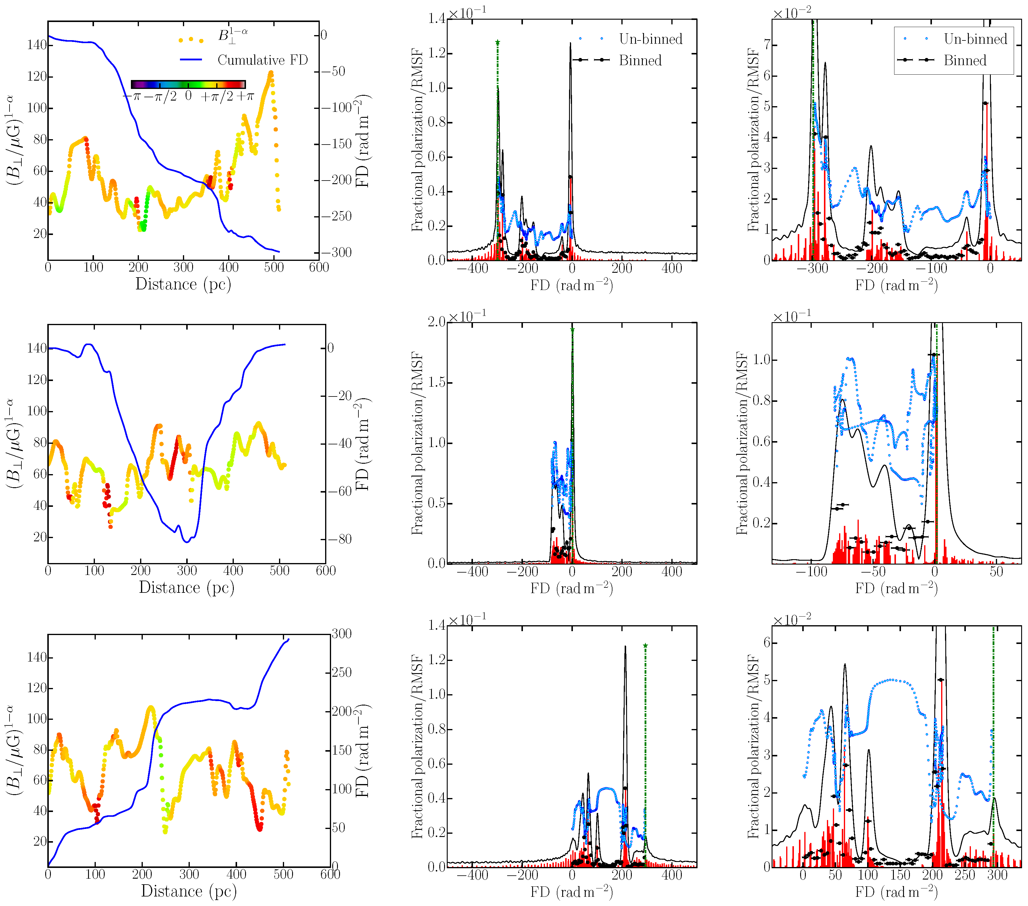
Here, we investigate the Faraday depth spectrum obtained by performing RM synthesis on the synthetic observations of MHD turbulence simulations and compare them to features in the variations of synchrotron emissivity and Faraday depth along the LOS. We will discuss these based on three LOS shown in Figure 11, as they are sufficiently representative of any other LOS and are therefore general representation of the results we will present. The left column displays $B_{\perp }^{(1-\alpha )}=B_{\perp }^{1.8}$ (for $\alpha =-0.8$), which is directly proportional to the linearly polarized synchrotron emissivity, at each position along the LOS and the Faraday depth from that position to the front of the domain (the side nearest to the notional observer). The emissivity-proxy fluctuates randomly about the expected mean value of ${\langle B_{\perp }\rangle }^{(1-\alpha )}={({\langle B_x\rangle }^2+{\langle B_y\rangle }^2)}^{\left(1.8\right)/2}\approx {\left(10\mathsf{\mu }\mathrm{G}\right)}^{1.8}$ (see Section 5), due to variation in $B_x,B_y$. This will translate into random structure in the amplitude of the Faraday depth spectrum. In Figure 11 (left column), $B_{\perp }^{(1-\alpha )}$ is colorized based on the intrinsic angle of polarization. Because of the strong $B_{\mathrm{ext}}$ along the x-direction, the polarization angle do not show strong fluctuations.

The Faraday depth of each point along the LOS shows a systematic non-random variation with position. This is because the Faraday depth is cumulative from a given position to the observer and the fluctuations in the magnetic field components are not delta-correlated. The correlation scale of $L_{\mathrm{c}}\sim 200$ pc is controlled by the forcing used to drive turbulence in the simulation: in these simulations the forcing scale is about 2.5 times smaller than the simulation box [43]. The driven turbulence contains fluctuations on all scales from $L_{\mathrm{c}}$ down to the dissipation scale (the separation between mesh points in this case), but the power-law behavior of the magnetic energy means that the field is strongest at $L_{\mathrm{c}}$. Therefore, the Faraday depth builds up systematically over path-lengths of roughly 200 pc. An interesting consequence of this is that, because the domain size is 512 pc, the Faraday depth variation along the LOS is not necessarily a monotonic function: the maximum magnitude of Faraday depth along a given LOS may not be that from the back to the front of the domain. If the domain was half the size, the Faraday depth variation would tend to be monotonic and if it were much bigger we would see multiple peaks and troughs in the Faraday depth variation. For domain sizes $L\gg L_{\mathrm{c}}$, FD variations would eventually appear to be random for $\langle B_{\parallel }\rangle$ = 0 μG. Thus, the form of the intrinsic Faraday depth variation depends on the number of turbulent cells along the LOS and does not necessarily look like a random function for shorter path-lengths. However, when combined with the variations in emissivity to produce the intrinsic Faraday depth spectrum the smoothness in $\mathrm{FD}$ along the LOS is not translated into a smooth spectrum.

The intrinsic polarized emissivity and Faraday depth combine to give the intrinsic Faraday depth spectrum shown by the blue points in the middle and right columns of Figure 11. Please note that these have been normalized to the maximum RM clean component, so only the relative variation contains useful information. Also shown in these panels is the spectrum obtained by RM synthesis and its clean components. The Faraday depth spectra are highly complex with multiple peaks and clean components referred to as a “Faraday forest” by Beck et al. [66]. These spectra are also clearly different from that obtained using delta-correlated Gaussian random field as an approximation to turbulence shown in Figure 10 (right-hand panel).

It is clear that the Faraday depth spectra are also very different from the intrinsic model spectra. RM synthesis tends to select a few strong peaks which are not always the FD along the entire LOS, nor are they closely related to features in the intrinsic polarized emission. This illustrates a fundamental difficulty in interpreting RM synthesis data. It may be wrong to interpret some of the narrow, high peaks as the action of a Faraday screen, or a Faraday thin component: a region in which there is no polarized emission, but which produces Faraday rotation. However, the corresponding left panels show that there is emission from all locations along the LOS.

A further difficulty in interpretation arises because the maximum absolute value of the Faraday depth along a LOS is not necessarily the Faraday depth through the entire box. The latter is shown by the green dash-dot line in the middle and right columns of Figure 11. For example, in the first row of Figure 11 the spectrum obtained by RM synthesis has strong peaks at $\mathrm{FD}\approx 0$ and $\mathrm{FD}\approx -300\mathrm{rad}{\mathrm{m}}^{-2}$ and looking at the left panel we see these correspond respectively to the emission generated at the front and back of the LOS. However, in the second row, the emission that produces the strong spectral peak near $\mathrm{FD}=0\mathrm{rad}{\mathrm{m}}^{-2}$ comes from emission from both the front and back of the layer. The Faraday depth through the entire layer is $\mathrm{FD}=1.67\mathrm{rad}{\mathrm{m}}^{-2}$ and the maximum along this LOS, $\mathrm{FD}\approx -80\mathrm{rad}{\mathrm{m}}^{-2}$ originates from the middle. There is no way yet that we are aware of, to reliably recover any of the true properties of the Faraday depth along the LOS from the Faraday depth spectrum alone. Images produced using the strongest spectral peak or the maximum absolute FD as proxies for some assumed property of a source, such as its intrinsic polarized emissivity or the total Faraday depth through it, may be misleading.

Pronounced peaks in the Faraday depth spectrum of a synchrotron-emitting medium can arise in two ways. A strong peak in emissivity from a region where the FD is changing slowly over a small distance will produce a narrow FD feature: an example is in the third row of Figure 11, where the strong emission from a distance between 190 and 210 pc, where the FD profile shows a step-like feature, produces the spectral peak at $\mathrm{FD}\approx 100\mathrm{rad}{\mathrm{m}}^{-2}$. Alternatively, when the FD is constant, or changing slowly over large distances, comparatively weaker emission builds up at this FD and results in a peak in the spectrum: in the third row of Figure 11 we see that $\mathrm{FD}\approx 200\mathrm{rad}{\mathrm{m}}^{-2}$ between the distance 250 and 450 pc along the LOS, producing a pronounced peak at this FD in the spectrum. Such a scenario can occur when the angle of the polarized emission is changing slowly with distance. In neither case does a strong peak in the spectrum result from a Faraday screen. While the origin of some spectral peaks can be approximately described by one of these mechanisms, there are also many peaks whose origin is not so simple and are discussed in the next section.

Multiple polarized components in Faraday depth spectrum is a natural consequence when the LOS passes through a few coherent scales. We believe, in the case when the LOS traverse through statistically large (asymptotically infinite) number of turbulent cells, Faraday depth spectrum similar to that obtained for delta-correlated random fields could perhaps be obtained. Given the typical driving scale of turbulence in the ISM, e.g., ∼50–100 pc when driven by supernova [42,68], and the typical length of LOS through the ISM of a few kiloparsec, achieving such a limit is highly unlikely. Unfortunately, the MHD simulations used here do not allow us to test this scenario. At present we are not aware of any reliable method which can be used to interpret Faraday depth spectra that originate in a turbulent, synchrotron-emitting region. Since turbulence and cosmic ray electrons are thought to be present throughout the ISM this problem requires careful investigation.

7.3. Comparing Clean Components to the Intrinsic Faraday Depth Spectrum

In Figure 11, the blue points showing the intrinsic emission at each Faraday depth are present between the main peaks in the spectra obtained by RM synthesis and RM clean. This is because, structures in FD are smoothed by the RMSF. In order to make a better comparison between the observed and intrinsic spectra it is important to consider the number of emitters in a given range of Faraday depths that is compatible with the resolution of the RMSF. We therefore binned synchrotron emissivities within a range of FD, with the bin-size determined by the RMSF. In our case, we used the bin-size $\Delta \mathrm{FD}=\mathrm{RMSF}/2$. The choice of this bin-size is motivated by the fact that we wanted to Nyquist sample the RMSF. This is equivalent to the sum of polarized intensities (${\epsilon }_{\mathrm{bin}}$) arising in the range $\mathrm{FD}\pm \Delta \mathrm{FD}/2$ and ${\epsilon }_{\mathrm{bin}}$ is given by,

$${\epsilon }_{\mathrm{bin}}\left(\mathrm{FD}\right)=\sum _{{\mathrm{FD}}_i}\epsilon \left({\mathrm{FD}}_i\right)\equiv N_{\mathrm{bin}}\langle {\epsilon }_{\mathrm{bin}}\rangle ,\mathrm{where}{\mathrm{FD}}_i\in \left[\mathrm{FD}-\Delta \mathrm{FD}/2,\mathrm{FD}+\Delta \mathrm{FD}/2\right].$$

(5)

Here, $N_{\mathrm{bin}}$ is the number of synchrotron-emitting elements within a FD bin computed from the simulation and $\langle {\epsilon }_{\mathrm{bin}}\rangle$ is the mean polarized synchrotron emissivity of that FD bin. As the intrinsic polarization angle of the synchrotron emission does not fluctuate strongly (as can be seen by the smooth color variation of the angle of the polarized synchrotron emission in the left column of Figure 11), simple addition of the polarized emissivities will not affect our conclusions. The black points in the middle and right columns of Figure 11 show ${\epsilon }_{\mathrm{bin}}$ located at the mean FD of the corresponding bin with the maximum value of ${\epsilon }_{\mathrm{bin}}$ normalized to the peak value of the FD clean components. It is clear from the middle and the right-hand panels of Figure 11 that the sum of polarized emission in FD bins captures the RM clean components, including their relative amplitudes, remarkably well.

Please note that strong ${\epsilon }_{\mathrm{bin}}$, and thus a peak in the Faraday depth spectrum can originate either due to—(1) strong emissivity at a location along the LOS (large $\langle {\epsilon }_{\mathrm{bin}}\rangle$), or due to (2) build up from several weaker emissions that have FD within $\pm \mathrm{RMSF}/4$ (large $N_{\mathrm{bin}}$). In fact, both these scenarios can occur along the same LOS. For example, in the top row of Figure 11, the peak near −300 rad m⁻² originates due to the first case, while the peak near 0 rad m⁻² is because of the second case. In the second row of Figure 11, the peak near 0 rad m⁻² is a consequence of the second case although the polarized emission in that FD bin originate from both front and back of the sightline. This clearly demonstrates that for a turbulent magneto-ionic medium which is simultaneously synchrotron-emitting and Faraday-rotating, a peak in the Faraday depth spectrum corresponds to the polarized emission summed roughly within $\pm \mathrm{RMSF}/4$, which necessarily may not arise from regions along the LOS that are spatially continuous. Therefore, special care must be taken when interpreting FD maps constructed through RM synthesis and relating them to the FD of the emitting volume, especially when the Faraday depth spectrum appears to be well resolved.

This brings out the important fact that even if a broad-band observation is sensitive to extended structures in Faraday depth space and can resolve them, as our synthetic observations are, the RMSF plays an important role in determining the amplitudes of the clean components. Moreover, when performing RM synthesis for diffuse emissions, sharp peaks in the Faraday depth spectrum that are consistent with the width of the RMSF do not necessarily imply the presence of a Faraday-rotating screen in the foreground of a synchrotron emitting volume.

Our investigation on Faraday depth spectra is based on a diffuse isothermal magneto-ionic medium as a representative Galactic ISM that contains transonic compressible turbulence. It is possible that the conditions of turbulence in different parts of the Galactic magneto-ionic medium could be of different type, including the distribution and direction of the regular magnetic fields. The conclusions regarding the origin of Faraday complexity and various peaks in the Faraday depth spectrum are expected to be general. However, depending on the spatial smoothness of the turbulent fields (for example, sub- or super-sonic turbulence) and strength of the regular fields, the peaks in Faraday depth spectrum could become smoother or merge together. In other words, the clumpyness of a well resolved Faraday depth spectrum could provide hints on the nature of turbulence in a magneto-ionic medium. Therefore, quantifications of the shape of Faraday depth spectrum beyond the recently used skewness and kurtosis [39] is necessary to be investigated to distinguish between different types of turbulent medium.

8. Conclusions

We have investigated in detail various features in Faraday depth spectra obtained from synthetic broad-band spectro-polarimetric observations in the frequency range 0.5 to 6 GHz sampled with 500 frequency channels. We have developed a new software package, COSMIC, wherein a user can freely choose from several possible options to generate synthetic observations. In this work the synthetic observations were obtained from MHD simulations of an isothermal, transonic, compressible turbulence in a plasma, similar to that observed in the Galactic ISM. For comparison, we have also studied the Faraday depth spectrum for a simple delta-correlated Gaussian random description of turbulent magnetic fields. We reach the following conclusions:

• For the MHD simulations used, Faraday depth varies smoothly with distance along the lines of sight due to spatially correlated structures in the magnetic field. Faraday depth varies on scales of ∼200 pc, similar to the driving scale of turbulence in the simulations used in this work.
• Strong Faraday depolarization at long wavelengths gives rise to canal-like small-scale structures in the polarized synchrotron emission. At the resolution of the MHD simulations used here, the polarized synchrotron emission below ∼1 GHz shows spatial variation at the scale of a few pixels that correspond to a few parsecs.
• For the choice of our frequency coverage, the synthetic observations are sensitive to structures extended up to ∼1250 rad m ⁻² in Faraday depth space and resolve them with RMSF of 10 rad m⁻². This allowed us to perform a high-resolution investigation of Faraday depth spectra. Faraday depth spectra for a medium containing Gaussian random magnetic fields that are delta-correlated are significantly different in structure as compared to those obtained from MHD simulations of a medium containing random magnetic fields that are spatially correlated. The latter is expected to be a closer representation of the diffuse ISM.
• Faraday depth spectra of individual sightlines through the MHD cube show a combination of narrow and broad features, which cannot be described as a linear combination of simple models that are typically used when polarization data are analyzed. The narrow structures are mostly consistent with the width of the RMSF containing a single FD clean component, typically considered to be a signature of a medium that is only Faraday-rotating, although the entire simulation volume is emitting synchrotron radiation.
• We find that modelling RM clean components of the Faraday depth spectrum as discrete emitters along a line of sight where at a physical distance, the synchrotron emissivity of the emitters is located at the Faraday depth to that distance does not represent the clean components obtained from RM clean.
• The clean components and their relative emissivities obtained from RM clean are well represented by the sum of polarized synchrotron emissivity in a Faraday depth bin of bin-size $\mathrm{RMSF}/2$.
• Since the Faraday depth spectrum depends on the interplay of the emissivity ${\epsilon }_{\mathrm{sync}}$ and the local Faraday depth, the complicated structures in Faraday depth can be explained as follows:

  –

  Strong sharp peaks in the spectrum can be produced due to reasons: (i) strong ${\epsilon }_{\mathrm{sync}}$ at a single FD, or, (ii) build up of weaker ${\epsilon }_{\mathrm{sync}}$ over a range of distance, not necessarily continuous, that have roughly constant FD, or whose FD lies in the range $\mathrm{FD}-\mathrm{RMSF}/4$ and $\mathrm{FD}+\mathrm{RMSF}/4$.

  –

  Broad spectral features are produced by: (iii) a gradient in FD at a constant ${\epsilon }_{\mathrm{sync}}$. Deviations from “constant” ${\epsilon }_{\mathrm{sync}}$ or FD produce sub-structure on (ii) and (iii).

• Our analysis shows that it is highly non-trivial to infer the Faraday depths, i.e., the integral 0.812 $\int n_{\mathrm{e}}{B}_{\parallel }\mathrm{d}l$ along the entire LOS, for a diffuse medium that emits synchrotron radiation if turbulent magnetic fields are dominant.

The turbulent magneto-ionic medium in a real astrophysical source is expected to be further complicated as compared to our simplified assumptions on its properties, such as a constant density of CREs with constant power-law spectral energy distribution, a constant ionization fraction of the neutral gas and above all, an ideal telescope response. In such scenarios, the generality of our investigation regarding peaks in Faraday depth spectrum originating due to accumulation of synchrotron emissivity within a range of FD determined by the RMSF is expected to hold true. The complication stems from the fact that whether the stronger synchrotron emissivity is a consequence of magnetic fields alone or due to variations in density of CREs or due to variations in their energy spectrum, will remain degenerate. In the presence of telescope systematics and noise, complications can be even more difficult to disentangle. With several upcoming broad-band spectro-polarimetric surveys of the diffuse Galactic emission and other surveys for extragalactic sources that are targeting major astrophysical questions, interpreting results obtained from spectro-polarimetric data analysis techniques in general, and RM synthesis technique in particular, requires improved statistical methods.