Solar and Galactic Magnetic Halo Structure: Force-Free Dynamos?

Department of Physics, Engineering Physics & Astronomy, Queen’s University, KIngston, ON K7L 3N6, Canada
Galaxies 2019, 7(2), 53; https://doi.org/10.3390/galaxies7020053
Submission received: 14 January 2019
/
Revised: 5 April 2019
/
Accepted: 18 April 2019
/
Published: 3 May 2019
(This article belongs to the Special Issue New Perspectives on Galactic Magnetism)
Abstract
:Magnetic fields may relax dissipatively to the minimum energy force-free condition whenever they are not constantly created or distorted. We review the axially symmetric solutions for force-free magnetic fields, especially for the non-linear field. A new formulation for the scale invariant state is given. Illustrative examples are shown. Applications to both stellar coronas and galactic halos are possible. Subsequently we study whether such force-free fields may be sustained by classical magnetic dynamo action. Although the answer is ‘not indefinitely’, there may be an evolutionary cycle wherein the magnetic field repeatedly relaxes to the minimum energy condition after a period of substantial growth and distortion. Different force-free dynamos may coexist at different locations. Helicity transfer between scales is studied briefly. A dynamo solution is given for the temporal evolution away from an initial linear force-free magnetic field due to both and terms. This can be used at the sub scale level to create a ‘delayed’ effect.
1. Introduction
Recently there has been some progress both in the measurement of galactic halo magnetic fields ([1,2]), and in the analytic theory of corresponding mean field galactic dynamos. A summary and references to earlier work can be found in [3], while recent analytic developments, using the assumption of scale invariance to treat the 3D problem, can be found in a series of papers [4,5,6]. These papers mostly start from the classical mean field theory [7], and study both axially symmetric dynamo fields and spirally bi-symmetric fields.
The scale invariant models succeed in predicting many of the new observations, some of which were known previously [8,9,10,11]), but some of which are only recently being detected [12,13] and represent genuine predictions. There is some evidence ([14], but see also [15]), that global magnetic fields may be axially symmetric as well as bi-symmetric. We focus on axially symmetric dynamos in this paper.
The strengths of even the organized (mean) magnetic fields can be surprisingly strong ([16]) being on average close to 10 G in the disc of spiral galaxies. It seems that these fields fall off in strength only gradually with height in the halo as is the case for NGC 891 ([17]), UGC10288 ([18]), and more recently ([19]). The consequent magnetic energy density in the galactic halo is of the same order or perhaps slightly greater than that of the hot halo gas. This suggests that, just as in the solar corona, the magnetic field may be force-free on average.
Dynamo action to produce such a force-free field is due either to a macroscopic velocity field or to a sub scale combination of turbulent generation and diffusion. The macroscopic velocity field would include large scale rotation and either halo inflow or outflow (e.g., [20]). Either the macroscopic flow or the sub scale turbulence may dominate the corresponding magnetic field. Consequently we expect dynamo action to gradually destroy the force-free aspect of the magnetic field. We do find this to be true in our arguments below after a finite time, starting from an initial force-free field. However, if indeed the field evolves to become energetically dominant, it could relax again to the force-free minimum energy condition with the dissipation of magnetic energy. Then the dynamo action would repeat and thus create a cyclic evolution of the galactic field, wherein there is always a period of force-free magnetic field.
In a force-free magnetic field, current must flow mainly parallel to the magnetic field. If there is a slight velocity difference between the ions and the electrons, winds of cosmic rays with small enough radius of gyration (that is a maximum energy) can produce such a current. Cosmic rays are produced in association with the sub scale turbulence driven by star formation and super novae that is necessary to the dynamo. This may be a mechanism for producing an initial nearly force-free field. These issues will appear more explicitly below, after our study of the geometry of force-free magnetic fields.
In any case in this paper we return to the notion of a force-free magnetic field and interacting dynamo ([7]). In the example studied by Moffat only the so called linear force-free magnetic field (a constant ‘current function’ that relates the current density to the field strength) was permitted and there was no velocity field. A simple formula for the time dependence of the field was given.
Our main interest is also in the time dependence of the linear force-free dynamo, but when a non-zero velocity field exists throughout the volume. This leads to a closed result for the time dependent linear force-free dynamo that should hold for a reasonable time. Some discussion of a non linear force-free dynamo is given when the velocity term is unimportant. There is also an approximate non force-free dynamo when it is the vector potential that satisfies a Beltrami condition. This also operates for a finite time.
The steady force-free magnetic field is also of interest, especially when applied to the magnetic fields in the halos of galaxies ([16,21]). The classic dynamo equation is not compatible with a steady force-free dynamo, so that any such field must be regarded as the result of more general magneto-hydrodynamics (MHD). This unknown flow must result in a dynamical stationary state wherein the Amperian force is unimportant. We give a simple example with incompressible Beltrami flow (i.e., the curl of the velocity is parallel to the velocity) provided the flow is also parallel to the magnetic field. The force-free field may be either linear or non linear, when we ignore its origin in this way.
The non linear (non constant current function) force-free magnetic can be studied analytically in axial symmetry. A separated 2D solution has been known in solar physics since the work of Low and Lou ([22] (see also [23,24]). We find that the basic equations can be expressed quite simply and generalize ([22]) to non separated solutions. We show also that the Low and Lou solutions are a sub-set of our scale invariant solutions, and make a detailed correspondence between the two approaches. We use both the general and the scale invariant formulations to present some intriguing examples that may apply either to solar active regions, or to the MHD ‘bubbles’ or ‘domes’ detected over the nuclei of spiral galaxies (e.g., NGC 3079 [25]). The polarized flux is seen to trace the nuclear outflow in the case of NGC3079. Recent applications of the Low and Lou solutions may be found in ([23]). Our scale invariant solutions generalize these possibilities slightly.
In Section 2 below we give our formulation of the non linear, axially symmetric, force-free, magnetic field, including a scale invariant version (see e.g., [5]). In the latter case a detailed comparison with ([22]) is given. In Section 3 we show illustrative examples. These are not applications to data, but are meant only to stimulate more detailed work based on the formulation given here. In Section 4 we consider when these non linear force-free magnetic fields can be maintained by classical dynamos. This section contains a formal description of magnetic helicity and a suggestion for how the magnetic helicity propagates in a two level system. The idea is pursued for linear force-free dynamos in Section 5.
The discussion of the linear evolving force-free dynamo with induced electric field is also found in Section 5. Application to the sub scale leads to a natural estimate for the velocity helicity that creates the dynamo. Interestingly, the consequent induced electric field is delayed in time.
A brief appendix considers the linear force-free steady dynamo in an approach compatible with the non linear examples and shows an example of the field.
2. Non Linear Force Free Magnetic Fields in Axial Symmetry
In this section we give a simple general approach to axially symmetric, non linear, force-free, magnetic field structure. This is followed by a scale invariant approach to the same problem that is new as far as I know. Examples of the possible non linear topologies are given for each approach.
2.1. General Formulation
We have to solve the equations
for and the magnetic field . We refer to the function as the parallel current function ( is a unit vector parallel to ). Note that q gives a reciprocal scale for the magnetic field so that if it is constant, no scale invariance is possible. If there is time dependence in q, it must derive from external dynamo and/or dynamic action.
Substituting the explicit expression for and from Equation (1) into Equation (2) gives an integral, based on the theorem for functional dependence, as
The function is arbitrary. It is clearly proportional to the current along the polar axis through a planar circular loop perpendicular to this axis, by Ampère’s law.
The radial and theta components of Equation (1) give directly the poloidal components of the magnetic field
to which we may add Equation (3) for the azimuthal field. The prime indicates differentiation of the function with respect to its argument.
However the components of must also satisfy the azimuthal component of Equation (1), which we have not yet used. On substituting Equations (3) and (4) into the azimuthal component we obtain an equation for q in the form
Here and q may be positive or negative (the latter corresponding to negative magnetic field linkages [7]). Because the function is arbitrary, a suitable choice allows the generation of analytic (or semi-analytic) non linear, force free fields; once the resulting equation for q is solved.
A (semi) analytic example wherein the vertical current density () varies as but increases with is
Equation (5) now implies
Setting
yields the simpler equation
for which a sum over separated solutions (i.e., modes) is easily found in terms of hypergeometric functions of x and power laws in r. The solution is restricted to be positive in the physical domain. We discuss this illustration in the example section. We note that it is a property of this treatment that q need not be separable in functions of x and r, so that Equation (5) gives the general non-linear, axially symmetric, force-free field in principle.
It is possible to write the equation for the parallel current function q when the axial current depends on any power of q. However the solution must be found numerically in general. It is more useful for these trial applications to study additional solutions that are restricted to be scale invariant. We consider these in the next sub-section for the first time to our knowledge.
2.2. Scale Invariant Non Linear Force Free Fields
The discussion of scale invariance requires a careful assessment of Dimensions. It is convenient to suppose that the magnetic field is divided by a constant , where is some arbitrary constant with the Dimensions of mass density. This will always be absorbed into arbitrary multiplicative constants in the solutions, but it allows us to take the Dimensions of the magnetic field to be equal to that of a velocity. It happens that this treatment is nearly equivalent to the separated solutions found in [22]. This will be discussed in detail in the next sub-section.
We proceed following the method described in [26] and elaborated in [27]. The scale invariant solutions are separated solutions, but they are found by applying a Lie symmetry in radius. The radial scale invariant symmetry reduces even non linear versions of Equation (5) to a non linear equation in . The method introduces reciprocal scales , in space and time Dimensions respectively. These allow us to write the key physical quantities in transformed expressions as
where the combination of scales in the exponential representations correspond to the space and time Dimensions of the physical quantities. The constant is introducd so that it does not appear subsequently in each of the components of .
Our immediate problem is to ensure that . A little trial and error shows that this is only possible if for some power p. But by our scale invariant ansatz (10) for q and j this requires
that is
We have set , which is the similarity class [26]. The time does not enter essentially into the force-free equations, but external influences can cause . However this cancels from Equation (5) in any case.
The case has no scale invariant solution. This implies that a global constant of Dimensions equal to specific angular momentum (or to kinematic viscosity) can not be associated with a scale invariant, force-free magnetic field.
The case has the field falling off fast enough with radius to maintain a finite field energy, but it poses a numerical problem in the form of a non linear, ordinary, second order differential equation. This reduction of the non linear force-free magnetic field was found many years ago using ad hoc scale invariance ([28]), but it was not known to fit a general scheme of scale invariance.
We treat the linear case in a notationally consistent fashion in the appendix. No spatial scaling is possible with q constant (i.e., the linear case), but the general solutions are familiar.
Once Equation (14) are solved for ,we obtain the magnetic field by using Equation (10) plus Equation (13) in Equations (3) and (4). The scale invariant part of the magnetic field becomes
The complete magnetic field () is given by the last expression in Equation (10). An arbitrary constant can multiply each of the field components. We look briefly at some examples of scale invariant and non scale invariant fields in Section 3. In the next sub-Section 2.3 we compare the results of this section to those of ([22]).
2.3. Low and Lou Solutions as Scale Invariance
A comparison of the basic functions in ([22]) to those used ( and ) in the scale invariant fields of the previous section allows the immediate identifications (Q, A and n are from [22])
However, a comparison of the expressions for the radial and poloidal magnetic field components found in ([22]) with those in Equation (16) shows that in our terms
for . This identifies
as well as implicitly Q and the constant . The expression for n in terms of the similarity class a always holds.
The case is not treated in ([22]) but this corresponds to our case as presented in Equation (14). In the formulation of Low and Lou this is a limiting case that is not readily treated. Our exceptional case that reduces to a potential field implies in Low and Lou, hence again reducing to a potential field.
Hence the full scale invariant approach has not replaced any of [22], but has only extended and clarified that formulation slightly. However the correspondence delivers a considerable bonus for the present paper. Low and Lou have studied at length the case , that is . Moreover they have solved an eigenvalue problem that shows that for this example there is a solution that is finite on the axis.
It should be remarked that the paper by Prasad, Mangalam and Ravindra ([24]) also extends the low and lou solutions in that they give (integral) eigen values that fit the boundary conditions for a wider range of n. The value of n is restricted to be rational, which is similar to the Dimensionally dictated value of a. They give extensive discussion of the application to solar physics.
Generally scale invariance can be expected to hold only over a limited range of spatial scale ([29]. There will always be divergence at for example. Even in polar angle, given the boundary condition as used in Low and Lou, the field tends to potential values on the axis () rather than the force free value. In our illustrative scale invariant examples we do not require the fields to hold over the the whole spatial range. In many cases the magnetic flux emanating from the axis is finite, even if the magnetic field diverges there.
One of the novelties of the full scale invariant approach is the identification of the parameter a as the similarity ‘class’. This means for example that when (i.e., ) one expects a global constant with Dimensions ([6]), where p is a positive or negative rational and L, T indicate length and time Dimensions. Such a global constant is coherent with the radial dependence of the magnetic field found in Equation (10), which is . This is because our magnetic field is scaled to have Dimensions , so that has the Dimensions indicated by a if .
From the above we infer only the obvious condition that the global constant must be assigned at one value of x, but the interpretation also suggests a rapid way of evaluating the physical character of other values of a. For example, when the constant has Dimensions , which requires a magnetic flux to be given at some x on taking . The interpretation of a (through the choice of p) is thus more or less evident in a purely magnetic system, but the presence of dynamics would add other parameters and possible interpretations. Thus the presence of a free-fall time adds an independent time Dimension and allows other interpretations of the global constant, such as the change of magnetic flux during a free-fall time.
3. Some Non Linear Force Free Dynamo Fields
3.1. Scale Invariant Examples
We refer to the first of Equation (14) and set the similarity class . This choice implies that a global constant with the Dimension of magnetic field exists, and this constant may be identified with the value of the field at fixed x. In the presence of dynamics, such a global constant is also consistent with a constant linear velocity such as that of the disc of a spiral galaxy.
Equation (10) shows that there is no radial dependence on the magnetic field and therefore . The current in the z direction is by Equation (13) and by Equation (10). Clearly there is no limit on the integrated energy of the field unless it is cut off at a finite radius. This cut requires boundary conditions connecting to an external potential field involving surface currents and forces that we will not consider here.
This has the solution
which must be positive in the domain of interest. By examining the limits at and we see that and should both be positive above the plane. The field does not recognize the plane as a boundary. Hence in any application to a spiral galaxy the field in the upper half plane should be reflected into the lower half plane with a sign change. This yields a dipolar symmetry across the equator. If the reflection is carried out without a sign change then one obtains quadrupolar symmetry across the disc plane. There has to be a surface current in the plane (volume current density integrated through the disc) to allow the dipolar boundary condition, but the two sides of the plane are quite disconnected with the quadrupolar symmetry. It is interesting to note that quadrupolar symmetry arises in the only analytic scale invariant MHD collapse solution ([27,30]).
The dipolar procedure maintains the normal component of the field continuous and changes the sign on the tangential components, while the quadrupole symetry reverses only the sign of the normal component. In a one-sided application, such as above an active region on the sun, the upper half plane solution suffices.
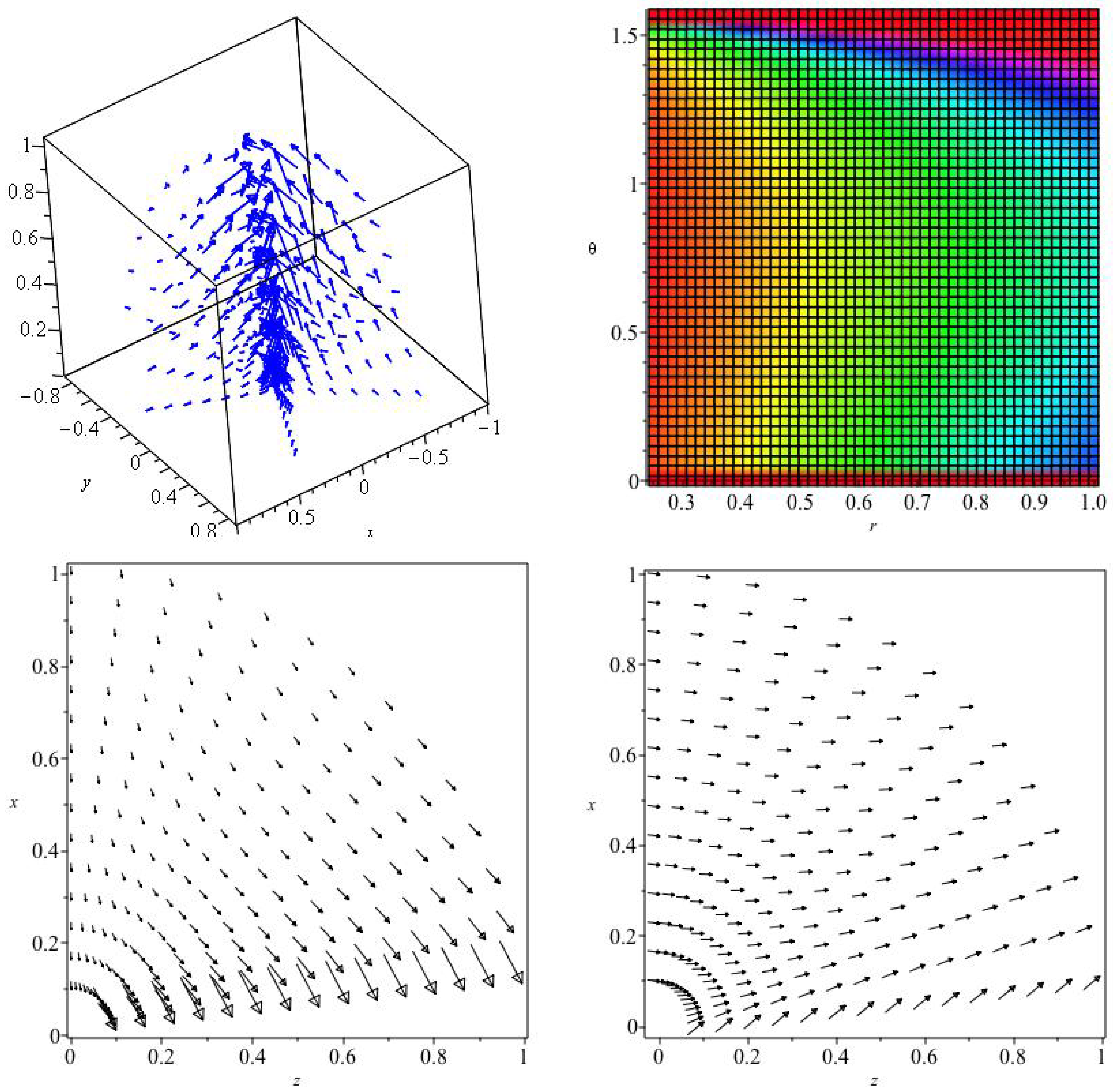
Solution (23) describes a magnetic field that is a function of angle only. We show some relevant properties in Figure 1. The three dimensional panel at upper left in the figure has the two independent solutions at equal amplitude . It shows dome like structure (cf NGC 3079 in [25]) with the field circling the polar axis. The polar circling (an axial current) is due to the solution while the dome structure can appear in both solutions. The panel at lower right shows a dominant solution with . The field is clearly ‘X shaped’ (cf [1]) in projection up to a limiting angle from the plane. No such behaviour occurs in the other limit where the solution dominates as is shown at lower left where .
The panel at upper right indicates the variation in the z axial current function for the case in the upper half plane. It varies substantially, declining by about a factor five starting from the axis in radius and by about a factor five at the polar angle extremes. However there are extensive ‘plateaus’ where q is roughly constant. We shall see that non linear force-free dynamo action may persist in such regions.
The total current flows parallel to the field lines by construction. The dome like structure, the X type field, the strong and variable axial current are the physical distinctions of this solution. The scale invariant field with class has no dependence on radius (although it varies strongly with x). However, dynamo action to evolve the field will be efficient mainly in the separate plateau regions. This can create an effective variation with radius. Such a magnetic field might be created by a nuclear jet (perhaps as in NGC3079), providing the jet creates a strong current on the polar axis.
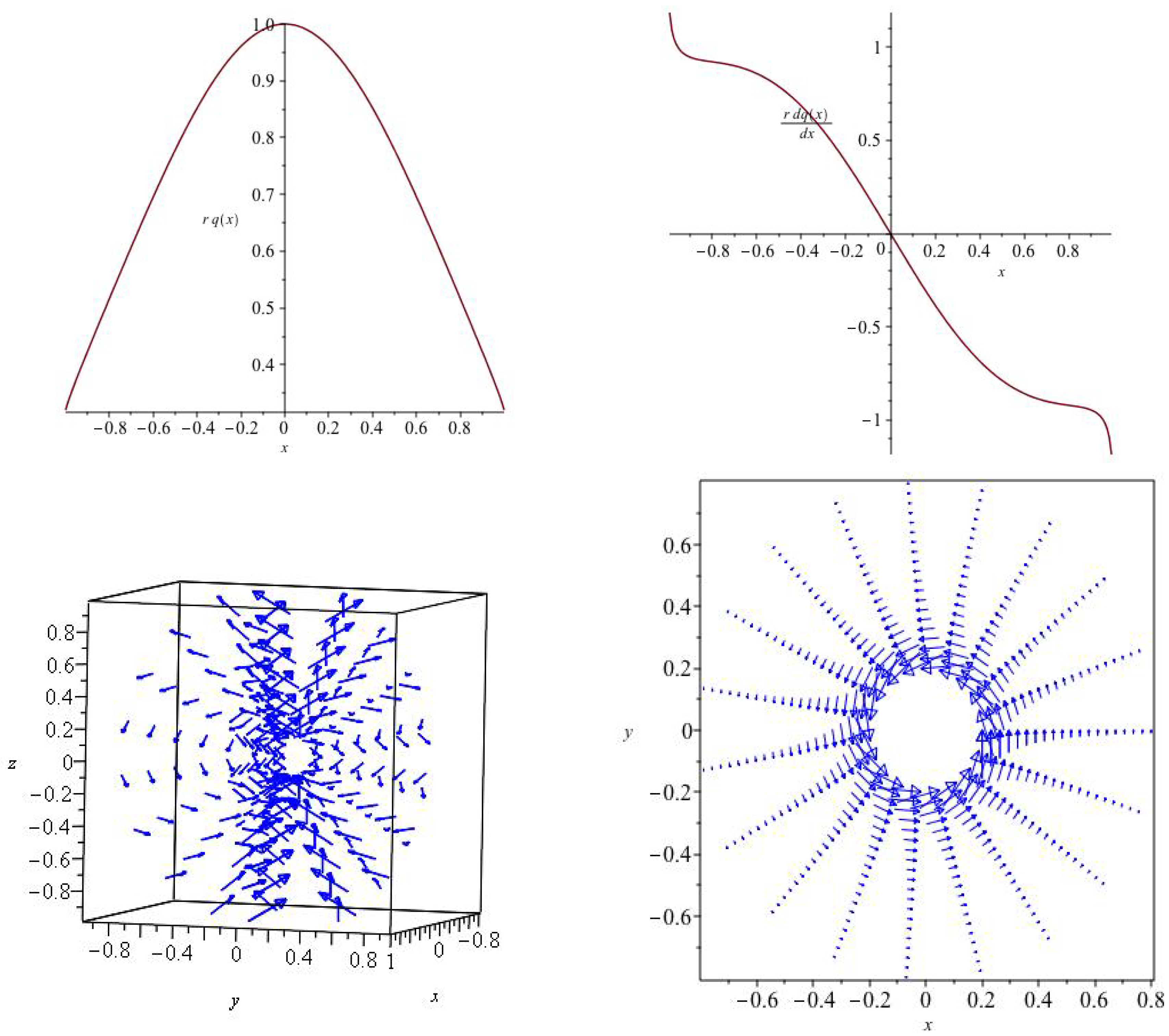
As perhaps a more physical example (the integrated field energy is finite without a boundary) we look briefly at the limiting case when . This choice implies a global constant with Dimensions , that is possibly a constant magnetic flux. The second of Equation (14) can be written as two linear equations and easily integrated numerically. We present only a two-sided example in Figure 2.
The upper left panel shows the variation of with the cosine of the polar angle. It is symmetric about the equator which implies that the current does not change sign on crossing the equator. The azimuthal and poloidal components of the magnetic field do not change sign, but the radial component does. This can be seen at upper right where the graph shows the angular derivative, d that is proportional to the radial magnetic field. This passes through zero on the equator in this symmetric solution.
At lower left the vectors of the magnetic field multiplied by are shown in three Dimensions. A projected ‘X type’ magnetic field might be observed near the polar axis in the polarized radio flux, but at larger angles the field is seen to be more dipolar in projection. There is however in addition an azimuthal component of the field, which the panel at lower right displays in the equator of the solution (where the radial field vanishes). This figure includes the radial inverse square decline with radius. Thus, only the X type field near the polar axis may be strong enough to be observed. The axis may also of course be the location of a double ‘jet’ (i.e., collimated) outflow.
3.2. Non Scale Invariant Example
We consider the non scale invariant example summarized in Equation (9). The general solution requires the application of boundary conditions in radius and poloidal angle. However a plausible solution is found when only one ‘mode’ is included, namely the term with the separation constant equal to 2. This gives a solution of Equation (9) in the form
where is the hypergeometric function. Note that this solution is completely symmetric under so long as below the plane. Only the radial magnetic field (and hence the radial current) will change sign due to the differentiation with respect to x. This will give double magnetic bubbles across the plane in a galaxy context. From Equation (8) we obtain . The magnetic fields follow from Equations (3), (4) and (6).
If the negative square root were extracted on crossing the plane, both and would change sign and we would have dipolar symmetry. It is not possible to have a global quadrupolar symmetry with this mode. However one can construct a quadrupolar solution, just as with the solution of the previous section, by reflecting the field above the plane in the plane without a sign change.
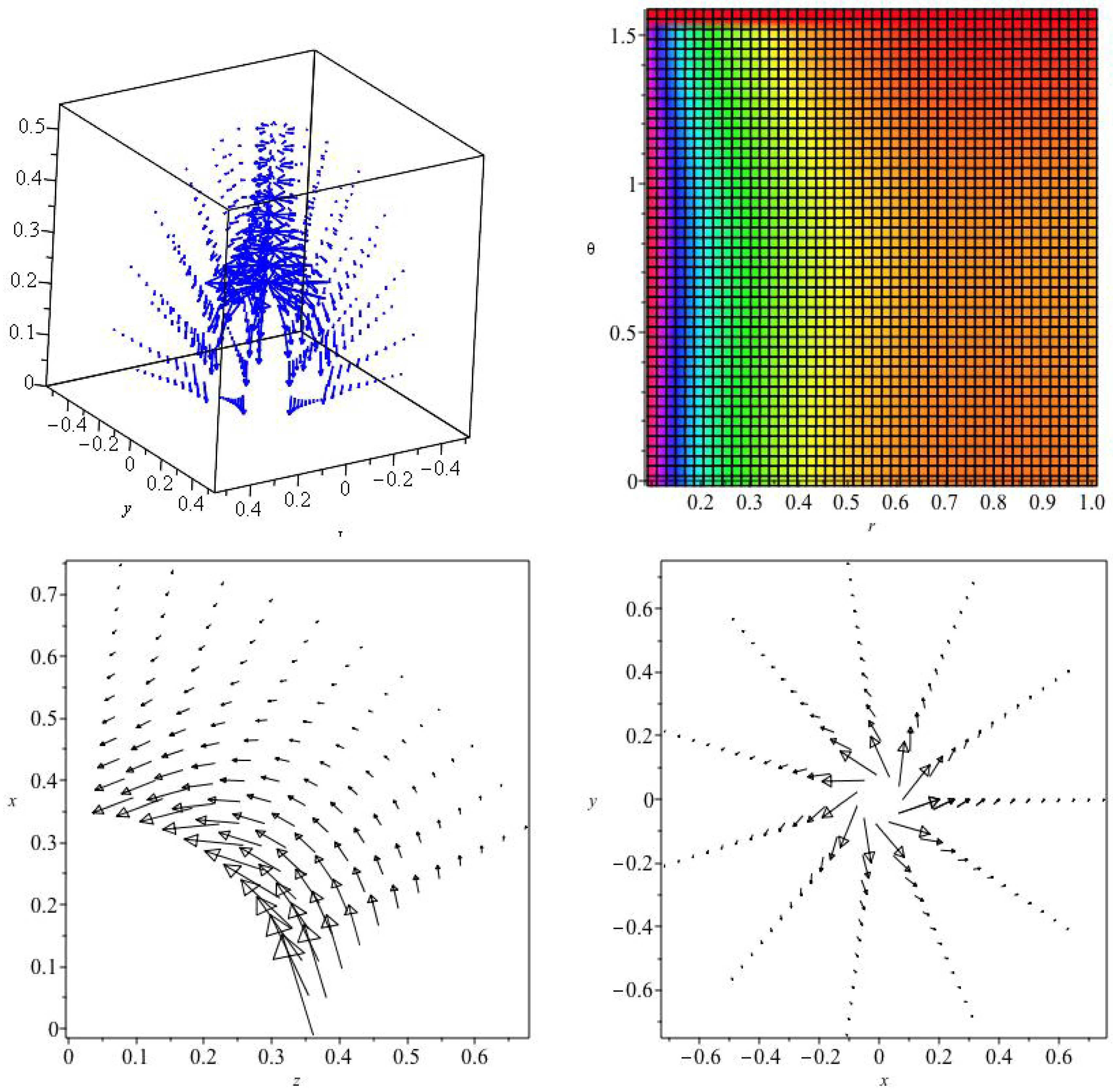
In Figure 3 we show several examples chosen more or less at random from the constants . Many other possibilities exist, including pure ‘X type’ fields, but such exploration is not the main purpose of this paper, which in these sections is mainly to demonstrate a useful formulation of the force-free magnetic field.
Although now we do not have scale invariance (note the strong variation in radius and polar angle), we do find similar dome structure and axial current in the upper left panel that may be associated with a jet. At upper right the reciprocal of the current function is plotted. The distribution of j gives an effective local spatial scale of the force free field. Once again there are plateaus, but j varies globally by about a factor 2. For the parameters chosen, the poloidal structure at lower left is purely dome like with no ‘X type’ behaviour. However a systematic study would show that there are many variations about this structure. The field vectors are shown reacting to the large axial current (also large spatial scale) at upper left and at lower right of the figure.
In the Appendix A Figure A1 we show one mode of a linear force-free magnetic field. There is no scale invariant solution, but the dome-like field structure is quite similar to scale invariant fields in that it produces the ‘dome like’ structure. It differs however by producing an axially symmetric azimuthal field that nevertheless oscillates in radius (c.f. [12]).
4. Non Linear Force-Free Dynamo
The force-free fields of the previous sections can only represent dynamo fields under certain conditions. We discussed these conditions qualitatively in the introduction. In this section we look at more specific cases.
4.1. Stationary Force-Free MHD Flow?
Equation (35) below shows that a steady force-free magnetic field is not compatible with a classic dynamo. This is evident because the two terms on the right of this equation can not cancel, being perpendicular vectors. If
then each term is zero and there is no classical dynamo action.1
Nevertheless a dynamical magnetized steady state can be maintained by a combination of pressure, gravity, viscosity, and inertial forces. The assumption of flow parallel to the magnetic field, in Equation (25) implies a wind of, or mixed with, cosmic rays. Accretion onto the galaxy along a magnetic field connected to its surroundings [4] is also possible.
Given some Ohmic dissipation we speculate that the magnetic field would be free to relax to its minimum energy, force-free state, because it is undistorted by the macroscopic velocity field, and there is no sub-scale dynamo action. The scalar function would be found dynamically as part of the dynamical relaxation process. If the conducting medium is incompressible, then is sufficient to keep constant on a field line, although it is not necessary.
A simple example is found when is constant in space. Then the steady flow is necessarily incompressible and is in fact Beltrami flow because , assuming the magnetic field is indeed given by Equation (1). The velocity helicity of this flow is .
The Navier-Stokes equations reduce in a dynamical stationary state with constant density and viscosity, Beltrami flow, and a force-free field to
where the Bernoulli function is
As usual p is pressure, is mass density, is a constant viscosity and is the gravitational potential. By taking the scalar and vector product of this equation with and recalling that according to the Beltrami condition, we can find useful expressions for the parallel and perpendicular components of the gradient of the Bernoulli function.
Any force-free magnetic field implies the corresponding by Equation (25) and constant, and vice versa. Hence, assuming an external gravitational potential, this equation gives the pressure distribution necessary for the dynamically steady state with Beltrami fluid flow (equal to the presence of a force-free magnetic field by our assumptions). Thus it is the pressure gradient that supports the magnetic field and so amplifies it by compression, in a kind of ‘hydro stationary dynamo’. Numerical simulations would be necessary to establish the existence of a physical time dependent path to such a configuration.
When q is constant, as for a linear force-free field, there is only a variation of the Bernoulli constant required parallel to and hence to . This is a case where the magnetic field acts as a conduit for the flow. It is at the other extreme where the magnetic field has become so strong that it dominates the other forces. It is force-free in that only a small part of the current flow need be perpendicular to the magnetic field. This appears to be the solar sun spot condition. Our example may not be taken seriously as a model for a galactic magnetic field, except near and in the galactic disc (e.g., [4]).
4.2. Time Dependent Force-Free Dynamo: I
We can reduce Equation (35) below when by taking the curl and assuming that u is spatially constant. So for simplicity we ignore the velocity here. A discussion including velocity will be included below in Section 5. The current procedure gives, after using Equation (1),
Here
where once again is the sub-scale helicity coefficient and is the turbulent viscosity.
We can write the solution for therefore as (The initial time derivative may be thought as a Lie derivative in time—e.g., [31] pp. 40–41)
where an arbitrary spatial function is absorbed into the initial force-free field.
However the argument fails at the next stage where we must establish that the dynamo field remains force-free as it evolves. Otherwise the entire formulation embodied in Equation (35) fails. Taking the curl once again, we see that the curl remains parallel to the magnetic field only if . However at the first differentiation, so that now only the linear dynamo with survives exactly. It is force-free with provided that the initial field is force-free with the same q. We develop this case further below.
It is of interest here to note explicitly how the general argument fails. It will be similar when velocity is included. The curl of Equation (30) gives
where we have used Equation (2), and is the unit normal to the plane defined by and in the direction of .
However by taking the dot product with we find the equation for the perpendicular component of the as
It thus diverges from zero faster than exponentially. However taking the ratio of the perpendicular component to the parallel component we find
Hence the magnetic field diverges from force-free field as becomes large. The characteristic time can be large, in regions where is sufficiently small. In fact it is readily shown for the scale invariant magnetic field that . When the second of Equation (14) allows us to write this as . Thus in that particular case the characteristic time is .
Until the characteristic time is reached, Equation (30) describes time dependent evolution by classical dynamo, of a non linear, force-free magnetic field. The initial field is a non linear force-free magnetic field as was studied in Section 2.1 and Section 2.2. The maximum amplification factor is therefore , which will vary from point to point.
Clearly the locally linear force-free dynamo field is maintained for the longest time, but there may be mainly step-wise variation in q between extended regions as in Figure 1 and Figure 3. In such a case we would have co-existing, but different, linear dynamos on different spatial scales.
As the field grows and diverges from the force-free condition in each region, the process may be quenched by due to a balance between generation and dissipation. Increased dissipation can cause a relaxation to a new average force-free field. The sub scale turbulence (part of the dissipation) will then restart the dynamo and a new cycle can begin in each region.
5. Time Dependent Force-Free Dynamo: II-Linear
We consider a linear force-free dynamo field that is driven by a macroscopic velocity field plus (isotropic) sub scale turbulence as manifested in the sub scale velocity helicity and diffusivity. The sub scale turbulence yields an helicity effect plus a diffusivity that might be on slightly different scales.
We recall the classical dynamo equation in the vector potential () form ([5,7])
where we neglect electrostatic fields. The definition of the electric field is just to recall basic assumptions. Combining this equation with Equation (1) assumed to hold initially, even for spatially non constant q, yields
We drop indications of the time derivative field at for brevity.
This last equation can also be written by defining a damped turbulent helicity, , as
where is the unit matrix, and the anti-symmetric matrix is ( refer to an orthogonal set of unit vectors).
Here is the fully anti-symmetric permutation symbol. Unfortunately Equation (36) does not in general guarantee the force-free evolution of an initial force-free magnetic field. We are then constrained to a force-free dynamo limited in time as in Section 4.2.
For a linear force-free field we may take 2 and so the Equation (36) for the temporal development of the force-free magnetic field becomes
The solution of this equation can be written in the operator form
where is an initial force-free field. Here we proceed purely formally with the operator algebra to find and verify the solution, but a somewhat more rigorous derivation of this solution can be found in either ([26]) or ([27]). The definition of an exponential matrix as an operator is a well established algebraic method.
At this point neither u nor need be uniform in space and both of them, plus the linear , may be arbitrary functions of time. However this arbitrariness does not gain us much in practice because these functions are unknown without extended dynamical considerations. Moreover, apart from the trivial , the time dependence does not help with maintaining the field of (39) force-free. We continue therefore with quantities constant in time.
Equation (39) (now with integrand constant in time although this is unnecessary) can be written explicitly because is anti-symmetric. Hence its exponential is given by the Rodrigues formula
where and varies in space. This leads us from Equation (39) to the expression
We have used a verifiable property of namely
and of course . Equation (41) represents a generalization of the discussion of force-free linear dynamos given in [7]). Note that nothing requires the initial force-free magnetic field to be axially symmetric, although that is the simplest version of the linear field.
Starting from an initial force-free magnetic field we see from Equation (41) that the first term continues to generate a force-free field so long as is spatially constant. We recall that requires only that
so that neither nor need be constant individually. Depending on the sign of finite u, there is either exponential growth or decay. Setting that is , identifies a typical dynamo number ([8]).
The more convoluted second term of Equation (41) will gradually deviate from the force-free condition as it grows, even if the modulus of the velocity v is constant. This term is small compared to the first term only if is small. Thus the dynamo generates a force-free field only for or e-folding times. This characteristic time may be nearly 100 Myr on a galactic scale . However even this estimate may be somewhat pessimistic.
One of the obvious physical questions is to ask how is the dynamo quenched? This can be achieved if, either the current source coefficients and/or the velocity, decay in time. We see that (as suggested in Section 4.2) will stop the exponential growth and leave only the small second term (for small ). So this is a form of quenching, achieved by cycling between distorted growth of a force-free field and subsequent relaxation.
Another possible example of quenching is to hold v constant in time and u constant (positive and uniform), but let in Equation (38). The detailed physics required is ignored here, but In an infinite dynamo with no characteristic scale, Dimensional analysis suggests that , where the velocity w might be either v or u or some combination of the two. This implies an increasing spatial scale of the field as it is generated.
Assuming this variation in time, the solution (41) holds, provided we replace t by and q by everywhere in the equation. The offending second term may now be kept small if is small. Here is an arbitrary time replacing , that is the time from which we start the dynamo. Formally, the amplitude of must absorb the factor .
We require then that for the evolution by force-free dynamo under these conditions. Unless w is substantially greater than v, we must have small, and hence is likely to be small. If in fact , then the growth stops abruptly.
The result of the operation is also of some interest. One finds (using physical components in spherical polars just for emphasis)
We note that
where is the initial induced electric field because is constant in time. Thus, according to Equation (41), the evolving field develops an electric field parallel to the magnetic field but it is a ‘delayed electric field’ relative to the current magnetic field. Even if the velocity were time dependent, Equations (39) and (41) together indicate that the electric field would depend on the past history of the flow plus the initial force-free linear field.
One should note that the scale of is not restricted. If we imagine that it is the turbulent scale, then we should set . In that case we conclude that the turbulent (helical in general) motion generates a ‘delayed’ electric field parallel to the magnetic field on the turbulent scale. This might be a candidate for an explicit ‘’ effect introduced on the mean field scale. It is an induced electric field similar to the electric field induced by the macroscopic flow. We speculate on this further in Section 5.2.
5.1. Non Force-Free Dynamo with Beltrami Potential
It is worth remarking that an additional use of our solutions of the force-free equations may be found by assuming that the vector potential obeys
that is we assume that the vector potential is a Beltrami vector field. Taking the Coulomb gauge , the earlier solutions for the force-free magnetic field apply directly to . However the magnetic field itself is no longer force-free because
The interesting application is to the classical dynamo Equation (34) which can be written as
without any constraints on u or . To make contact with the results of Section 5 we write this as
where
This means that the solution for is given by Equation (41), but with replacing , replacing q, replacing v and replacing . The field must be found subsequently from the curl of this expression.
Unfortunately this solution does not guarantee the Beltrami nature of , which is the same problem that we had with the force-free magnetic dynamo evolution. It requires to be small and to be constant to remain a good approximation. Of course we can set the net velocity to be zero, but then there is no ‘omega’ dynamo because the velocity field diffuses away.
5.2. Effect?
We imagine an initial two scale linear force-free magnetic field. The large scale is labelled while the sub scale is labelled . On the sub scale there will be no velocity helicity and no diffusivity so that . The ‘dynamo equation’ on the sub scale will be, on recalling Equation (35), setting , and taking total vectors on the scale
We take total quantities and .
From the previous section we know that the solution for the magnetic field can be written, at least initially, as
where
and
In this last expression, the average is over the large scale spatial region.
Formally then we obtain an estimate of the alpha effect by introducing the coefficient as
This value of can in principle now be used in Equation (38) to write an equation for the evolving force-free mean field while using a time varying sub scale helicity . To achieve a similar expression for the diffusivity would require considering two level dynamical equations. However Dimensional analysis suggests . This all suggests setting given our estimate for . The behaviour is only modulated slightly by the function F, when the argument is small.
Our considerations can not claim to probe the fundamental theory of dynamo action, for which the literature is rather vast (e.g., [32]). This is particularly the case because the assumption of a force-free field gradually fails in time. However it is remarkable that a simple model based on the evolution by a classic force-free dynamo reaches a conclusion similar to that inferred by ([33,34]). The important conclusion is that the delayed induced electric field, due to both turbulent and mean flow and field, provides a source for the current dynamo field. This means that the current dynamo field, in a galaxy for example, may depend on both earlier seed fields and ‘seed motion’.
Our next section discusses briefly helicity and its possible cascade between spatial scales. In a brief appendix we give the formulation of a linear force-free magnetic field in a form compatible with our discussion of the non-linear force-free field.
6. Force-Free Magnetic Helicity
The magnetic helicity transfer and conservation is an important indicator of the physics operating in a magnetic dynamo (e.g., [7,35]). The velocity helicity is fundamental to the turbulent dynamo. It is worth considering how this operates in a force-free magnetic field, but we begin with a general discussion of magnetic helicity, provided as always there is no electrostatic field.
The basic classical dynamo Equation (34) for a generated magnetic field is comprised of Faraday’s equation (no electrostatic field) and the assumed electric field in the forms
This allows us to write the time dependence of the magnetic helicity using only Faraday’s law as
We have in addition the identity ), and hence we find
We proceed by inserting the classical dynamo version of the electric field (34) into the first term of Equation (58), to obtain quite generally
If finally the magnetic field is force-free, this result becomes
The first term in this time dependence is proportional to the production of magnetic energy by the effect at the macroscopic scale minus the diffusive loss. The second term is more subtle. However for a linear force-free field . We see consequently that the second term is proportional to the divergence of the Poynting flux. Integrated over a closed volume. the resulting Poynting flux will vanish integrated over the bounding surface, provided that there is no net energy loss from the volume.
The spatial variation of the magnetic helicity h is
where in the force-free case. In a region of linear force-free magnetic field , and so this becomes
From this result and Equation (60) one can construct a convective derivative which allows in principle to extend the helicity over the whole space from a set of boundary values. For a non force-free magnetic field we require Equations (59) and (61). Rather than regard these results as new equations for the field, the magnetic field is found from Equation (56), after which the results of this section give the local temporal and spatial variation.
In view of the usual split between the sub scale and the mean field scale, it is of interest to consider both scales as force free and individually linear. If the mean field scale is labelled and the sub scale then
where the average is over the macroscopic field scale and the sub scale average is assumed to vanish when multiplying a macro scale quantity. If both scales are force-free and linear, then substituting for on each scale gives
Together with Equation (60) we see that when the integrated conserved total helicity implies a conserved balance between the sub scale and mean field scale helicity. Equivalently the balance is between the magnetic energy per unit area on each scale. Such balance is to be expected in standard dynamo theory.
7. Discussion and Conclusions
We have done two quite separate things in this paper, of which the second in Section 5 is perhaps the most original. In that section we give the solution for of an evolving linear force-free magnetic field when the velocity field is quite general. One finds (see Equation (41)) that the field develops an electric field parallel to the magnetic field but that it is delayed in time. That is, the electric field induced by the initial velocity and magnetic fields is parallel to the current magnetic field after a time t. The velocity field may be either sub scale and turbulent, or it may be the mean flow.
In a sub section of this part we use the two scale force-free dynamo to estimate the sub scale effect. This follows from the general solution for the dynamo evolution of the linear field. The time dependence of the effect declines essentially as , which resembles a scale invariant result for the classic dynamo ([6]).
Unfortunately, even evolving from an initial force-free magnetic field the field does not remain force-free. Dynamo evolved force-free fields are thus transitory and perhaps cyclic, assuming dissipative relaxation to the minimum energy state. The lifetime of the force-free phase can nevertheless be quite long. This evolving/ dissipating cyclic behaviour holds both for the linear and for the non linear force-free dynamo evolution. It is a type of ‘quenching’ the dynamo, but in an oscillatory manner.
In summary, the solution (41) can serve as an approximation to the solution of Equation (38) for spatially varying q that is sufficiently slow. Figure 1 and Figure 3 show in the relevant panels that q can in fact be slowly varying over large spatial regions.
In an earlier extensive Section 2 we have studied the axially symmetric non-linear force-free magnetic field by itself, because of possible solar corona applications [22,36] or galactic halo applications (e.g., [5]). The solutions in arbitrary geometry are notoriously difficult to find, but Equation (5) gives a simple formulation for the axially symmetric force-free field. Examples are given in Section 3.2, although there are parameters left unexplored and only one mode in a series is considered. Boundary conditions are required in any specific application. Interesting dome structure is shown in Figure 3 that resembles some structures over galactic nuclei (e.g., NGC3079, [25]), or over solar active regions.
In this context a new formulation is the scale invariant form of the non-linear force-free field Equation (14) studied in Section 2.2 and Section 3.1. This symmetry in addition to the axial symmetry reduces the problem to an ordinary differential equation. Special choices of the similarity class a should reflect the Dimensions of global constants of the problem ([6]). When is taken as an example, it implies a global constant with the Dimensions of macroscopic velocity, possibly rotational or inflow/outflow.
The choice implies a global constant with the Dimensions of magnetic flux (because the field has been scaled to have the Dimensions of velocity). This example (because there is an inverse square radial dependence in the field) keeps the magnetic energy finite even in an infinite volume. The parameters chosen to illustrate this example are somewhat arbitrary, but they present ‘dome-like’ behaviour with an axial ‘jet’ just as do the non scale invariant solutions (e.g., Figure 2). The ‘X type’ magnetic field structure can be seen in the scale invariant case with (1).
In Section 2.3 we recognized that the earlier work of Low and Lou ([22]) was in fact a scale invariant set of the axially symmetric soutions. In that section we give a detailed comparison between that work and our own. We show that the formal scale invariant theory only extends slightly their results to include the () solution. The concept of the similarity class a is also new.
Force-free magnetic fields have a scale built in as . We have used this idea in Section 5 to consider the effect, as was remarked above. In this context we have also summarized the evolution of magnetic helicity for the classical dynamo field. We demonstrated that two coupled force-free levels conserve helicity as an exchange between them. The conserved force-free magnetic helicity is proportional to the magnetic energy density.
Steady initial force-free magnetic fields are inconsistent with classical dynamo evolution. Steady force-free fields (linear and non linear) can exist passively in a macroscopic hydrodynamical flow in which other forces dominate. In our simple example the velocity is parallel to the force-free magnetic field and comprises an incompressible Beltrami flow. This ‘hydrodynamic dynamo’ is thus a result of forces (e.g., gravity and pressure) driving the dynamics and which dominate any Ampèrian force as the field is established.
There is another limit in MHD flow when the field is so strong that it dominates other forces and acts as a conduit for the flow. It is force-free now in the sense that a small Ampèrian force serves to dominate other forces.This appears to happen above sun spots and may happen in parts of spiral galaxies. Nuclear outflows or ‘champagne flows’ may be involved.
In an appendix we give a formulation for the familiar linear force-free magnetic field, which is notationally coherent with our non linear examples. We show an example in Figure A1 for a single mode. The dome-like structure and spiralling field structure on cones is common to many solutions. By contrast projected ‘X-type’ fields do not occur.
Funding
This research received no external funding.
Acknowledgments
I would like to thank Andrew Fletcher for stimulating this discussion although he is not otherwise guilty. My wife J. A. Irwin always does her best to suppress my more literary meanderings.
Conflicts of Interest
The author declares no conflict of of interest.
Appendix A. Linear Force-Free Magnetic Field
Equation (1) of the text when q is constant has well known solutions. It may be helpful in using Equation (41) to have a formulation similar to that for the non linear force-free magnetic field. More complicated methods must be used in the absence of axial symmetry so we proceed with that assumption in spherical polar coordinates. In that case the field is given by
and the equation to be solved is
With q constant there can be no scaling symmetry in space.
A simple solution with separation constant equal to 2 is
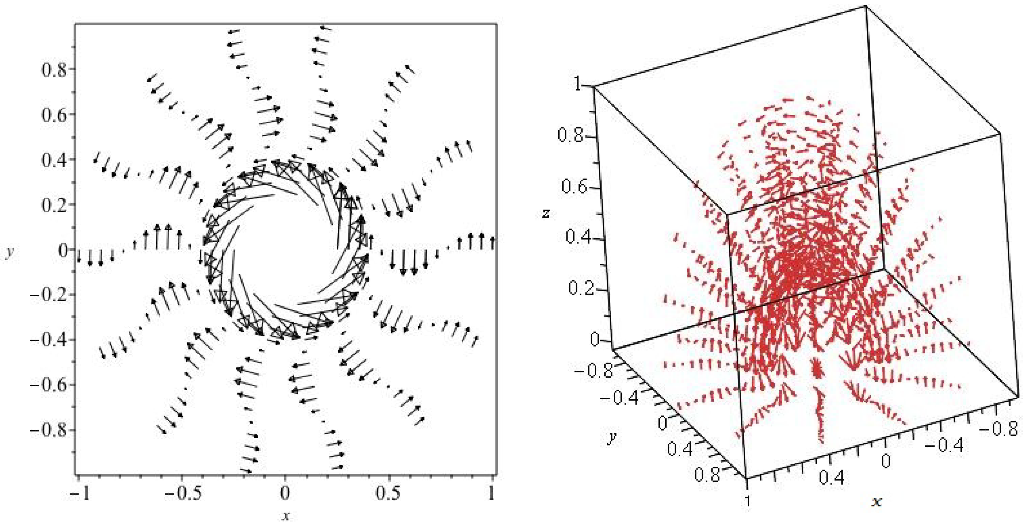
where F is the hypergeometric function and . Interesting behaviour when the current is large ( ) is shown in Figure A1. Only a simple dome like field appears with small q, typically .
The three dimensional vector plot shows the complexity of the force-free field. The vectors in the dome like structure reverse direction several times and there is strong winding of field lines near the axis. The field line plot on the cone at to the axis illustrates the toroidal winding as well as the reversal in azimuthal direction.
Depending on the velocity field, the evolved force-free magnetic field of Equation (44) will be greatly distorted. It is clear that there are many parameters, namely the five in the figure plus u and in the text, that may be adjusted for experimentation.
Figure A1.
At upper right the linear force-free field is shown in three dimensions with . The field winds around the axis and the dome like structure oscillates in direction. The radius has been integrated from to 1. On the left the toroidal field is shown wound on a cone with opening angle of relative to the polar axis. The radius is integrated over . Reversing toroidal field lines are evident.

References
- Krause, M. Magnetic Fields in Spiral Galaxies. Available online: https://www.mpifr-bonn.mpg.de/966263/Session-V.pdf (accessed on 26 April 2019).
- Wiegert, T.; Irwin, J.A.; Miskolczi, A.; Schmidt, P.; Mora, S.C.; Damas-Segovia, A.; Stein, Y.; English, J.; Rand, R.J.; Santistevan, I.; et al. CHANG-ES.IV-Radio continuum emission of 35 edge-on galaxies observed with the Karl G. Jansky Very Large Array in D configuration-data release 1. Astron. J. 2015, 150, 81. [Google Scholar] [CrossRef]
- Klein, U.; Fletcher, A. Galactic and Intergalactic Magnetic Fields; Springer: Basel, Switzerland, 2015. [Google Scholar]
- Henriksen, R.N.; Irwin, J.A. Magnetized galactic haloes and velocity lags. Mon. Not. R. Astron. Soc. 2016, 458, 4210–4221. [Google Scholar] [CrossRef]
- Henriksen, R.N. Magnetic spiral arms in galaxy haloes. Mon. Not. R. Astron. Soc. 2017, 469, 4806–4830. [Google Scholar]
- Henriksen, R.N.; Woodfinden, A.; Irwin, J.A. Exact axially symmetric galactic dynamos. Mon. Not. R. Astron. Soc. 2018, 476, 635–645. [Google Scholar] [CrossRef]
- Moffat, H.K. Magnetic Field Generation in Electrically Conducting Fluids; Cambridge University Press: Cambridge, UK, 1978. [Google Scholar]
- Brandenburg, A. Simulations of Galactic Dynamos. In Magnetic Fields in Diffuse Media; Springer: Basel, Switzerland, 2015; pp. 529–555. [Google Scholar]
- Moss, D.; Sokoloff, D. The coexistence of odd and even parity magnetic fields in disc galaxies. Astron. Astrophys. 2008, 487, 197–203. [Google Scholar]
- Moss, D.; Beck, R.; Sokoloff, D.; Stepanov, R.; Krause, M.; Arshakian, T.G. The relation between magnetic and material arms in models for spiral galaxies. Astron. Astrophys. 2013, 556, 147–158. [Google Scholar] [CrossRef]
- Sokoloff, D.; Shukurov, A. Regular magnetic fields in coronae of spiral galaxies. Nature 1990, 347, 51–53. [Google Scholar] [CrossRef]
- Mora Partiarroyo, S.C. Deep Radio Continuum Study of NGC 4631 and Its Faraday Tomography. Ph.D. Thesis, Bonn Universität, Bonn, Germany, 2016. [Google Scholar]
- Woodfinden, A.; Henriksen, R.N.; Irwin, J.A. Exact spirally symmetric galactic dynamos. Mon. Not. R. Astron. Soc. 2018. submitted. [Google Scholar]
- Mao, S.A.; Carilli, C.; Gaensler, B.M.; Wucknitz, O.; Keeton, C.; Basu, A.; Beck, R.; Kronberg, P.P.; Zweibel, E. Detection of microgauss coherent magnetic fields in a galaxy five billion years ago. Nat. Astron. 2017, 1, 621–626. [Google Scholar] [CrossRef]
- Terral, P.; Ferrière, K. Constraints from Faraday rotation on the magnetic field structure in the Galactic halo. Astron. Astrophys. 2017, 600, 29–52. [Google Scholar] [CrossRef]
- Beck, R. Magnetic fields in Spiral Galaxies. Annu. Rev. Astron. Astrophys. 2016, 24, 459–497. [Google Scholar] [CrossRef]
- Mulcahy, D.D.; Horneffer, A.; Beck, R.; Krause, M.; Schmidt, P.; Basu, A.; Chyzy, K.T.; Dettmar, R.-J.; Haverkorn, M.; Heald, G.H.; et al. Investigation of the cosmic ray population and magnetic field strength in the halo of NGC891. Astron. Astrophys. 2018, 615, A98. [Google Scholar] [CrossRef]
- Irwin, J.A.; Krause, M.; English, J.; Beck, R.; Murphy, E.; Wiegert, T.; Heald, G.; Walterbos, R.; Rand, R.J.; Porter, T. CHANG-ES-III. UGC10288-An edge-on galaxy with a background double lobed radio source. Astron. J. 2013, 146, 164. [Google Scholar] [CrossRef]
- Krause, M.; Irwin, J.; Wiegert, T.; Miskolczi, A.; Damas-Segovia, A.; Beck, R.; Li, J.-T.; Heald, G.; Mueller, P.; Stein, Y. CHANG-ES. IX, Radio scale heightsand scale lengthsof a consistent sample of 13 spiral galaxies seen edge-on and their correlations. Astron. Astrophys. 2018, 611, A72. [Google Scholar] [CrossRef]
- Heesen, V.; Krause, M.; Beck, R.; Adebahr, B.; Bomans, D.J.; Carretti, E.; Dumke, M.; Heald, G.; Irwin, J.; Koribalski, B.S.; et al. Exploring the making of a galactic wind in the starbursting dwarf irregular galaxy IC10 with LOFAR. Mon. Not. R. Astron. Soc. 2018, 476, 1756–1764. [Google Scholar] [CrossRef]
- Beck, R. Magnetic Fields in the nearby spiral galaxyIC342. Astron. Astrophys. 2015, 578, 27. [Google Scholar]
- Low, B.C.; Lou, Y.Q. Modeling solar force-free magnetic fields. Astrophys. J. 1990, 352, 343–352. [Google Scholar] [CrossRef]
- Mangalam, A.; Prasad, A. Topological and statistical properties of nonlinear force-free fields. Adv. Space Res. 2018, 61, 738–748. [Google Scholar] [CrossRef]
- Prasad, A.; Mangalam, A.; Ravindra, B. Separable solutions of force-free spheresand applications to solar active regions. Astrophys. J. 2014, 786, 81. [Google Scholar] [CrossRef]
- Irwin, J.A.; Schmidt, P.; Damas-Segovia, A.; Beck, R.; English, J.; Heald, G.; Henriksen, R.N.; Krause, M.; Li, J.-T.; Rand, R.J.; et al. CHANG-ES-VIII. Uncovering hidden AGN activity in radio polarization. Mon. Not. R. Astron. Soc. 2017, 464, 1333–1346. [Google Scholar] [CrossRef]
- Carter, B.; Henriksen, R.N. A systematic approach to self-similarityin Newtonian space-time. J. Math. Phys. 1991, 32, 2580–2597. [Google Scholar] [CrossRef]
- Henriksen, R.N. Scale Invariance: Self-Similarity of the Physical World; Wiley-VCH: Weinheim, Germany, 2015. [Google Scholar]
- Henriksen, R.N. Force-Free magnetic fields of current interest. Astrophys. Lett. 1967, 1, 37–38. [Google Scholar]
- Barenblatt, G.I. Scaling, Self-Similarity, and Intermediate Asymptotics; Cambridge Texts in Applied Mathematics; Cambridge University Press: Cambridge, UK, 1996. [Google Scholar]
- Aburihan, M.; Fiege, J.; Henriksen, R.N.; Lery, T. Protostellar evolution during time-depemdent anisotropic collapse. Mon. Not. R. Astron. Soc. 2001, 326, 1217–1227. [Google Scholar] [CrossRef]
- Bluman, G.W.; Kumei, S. Symmetries and Differential Equations; Applied Mathematical Sciences; Springer: New York, NY, USA, 1989. [Google Scholar]
- Brandenburg, A. Advances in mean-field dynamo theory and applications to astrophysical turbulence. J. Plasma Phys. 2018, 84. [Google Scholar] [CrossRef]
- Chamandy, L.; Subramanian, K.; Shukurov, A. Galactic spiral patterns and dynamo action-I: A new twist on magnetic arms. Mon. Not. R. Astron. Soc. 2013, 428, 3569–3589. [Google Scholar] [CrossRef]
- Reinhardt, M.; Devlen, E.; Rädler, K.-H.; Brandenburg, A. Mean-field dynamo action from delayed transport. Mon. Not. R. Astron. Soc. 2014, 441, 116–126. [Google Scholar] [CrossRef]
- Blackman, E.G. Magnetic Helicity and large scale magnetic fields: A primer. Sol. Stellar Astrophys. 2015, 188, 59–91. [Google Scholar] [CrossRef]
- Bonanno, A.; Del Sordo, F. Analytic mean-field α2-dynamo with a force-free corona. Astron. Astrophys. 2018, 605, A33. [Google Scholar] [CrossRef]
Figure 1.
At upper left the magnetic field vectors in 3d are shown for the Solution (23) with . At upper right we show the current function above the plane. From orange to green this function varies downwards by about a factor 5 and the same variation upwards holds from green to blue, At lower left the field vectors are shown in a poloidal cut with , while at lower right the poloidal cut is shown for .

Figure 2.
At upper left we show as a function of . We have chosen the symmetric example with and the derivative equal to zero. The derivative is shown at upper right. The field vectors, multiplied by , are shown above and below the equatorial plane at lower left. The radius runs from to in arbitrary Units although this dependence has been removed from the magnetic field. At lower right the true field vectors are shown in the equatorial plane over the same range in radius. The radial component passes through zero in this plane.

Figure 3.
At upper left we show a three dimensional set of field vectors for the parameter set , which set applies to all of the panels in this figure. The radius runs only from to at upper left in order to show inner and outer features. At upper right we show the vertical current function. It declines in radius from the axis by about a factor 2 at , but there are lower regions near the equator and near the axis for . The panel at lower left shows vectors in the poloidal plane with the z axis horizontal. The radius runs only from to . Near the axis the field becomes nearly toroidal due to the strong axial current. The circulating field appears in the figure at lower right at small radius, although the radius runs from to . This is actually the radius along the cone with opening angle projected along the polar axis onto the equatorial plane. Hence the radius along the cone is twice as large as that shown.

| 1 | We have defined as the sub-scale helicity coefficient and as the turbulent viscosity. |
| 2 | This is another condition for a force-free magnetic field but it does not guarantee that behaviour unless is solved for. |
© 2019 by the author. Licensee MDPI, Basel, Switzerland. This article is an open access article distributed under the terms and conditions of the Creative Commons Attribution (CC BY) license (http://creativecommons.org/licenses/by/4.0/).
Share and Cite
MDPI and ACS Style
Henriksen, R. Solar and Galactic Magnetic Halo Structure: Force-Free Dynamos? Galaxies 2019, 7, 53. https://doi.org/10.3390/galaxies7020053
AMA Style
Henriksen R. Solar and Galactic Magnetic Halo Structure: Force-Free Dynamos? Galaxies. 2019; 7(2):53. https://doi.org/10.3390/galaxies7020053
Chicago/Turabian StyleHenriksen, Richard. 2019. "Solar and Galactic Magnetic Halo Structure: Force-Free Dynamos?" Galaxies 7, no. 2: 53. https://doi.org/10.3390/galaxies7020053
Note that from the first issue of 2016, this journal uses article numbers instead of page numbers. See further details here.