Revisiting the Equipartition Assumption in Star-Forming Galaxies

Abstract

Energy equipartition between cosmic rays and magnetic fields is often assumed to infer magnetic field properties from the synchrotron observations of star-forming galaxies. However, there is no compelling physical reason to expect the same. We aim to explore the validity of the energy equipartition assumption. After describing popular arguments in favour of the assumption, we first discuss observational results that support it at large scales and how certain observations show significant deviations from equipartition at scales smaller than ≈$1\mathrm{kpc}$, probably related to the propagation length of the cosmic rays. Then, we test the energy equipartition assumption using test-particle and magnetohydrodynamic (MHD) simulations. From the results of the simulations, we find that the energy equipartition assumption is not valid at scales smaller than the driving scale of the ISM turbulence (≈$100\mathrm{pc}$ in spiral galaxies), which can be regarded as the lower limit for the scale beyond which equipartition is valid. We suggest that one must be aware of the dynamical scales in the system before assuming energy equipartition to extract magnetic field information from synchrotron observations. Finally, we present ideas for future observations and simulations to investigate in more detail under which conditions the equipartition assumption is valid or not.

1. Introduction

Magnetic fields are an important component of the interstellar medium (ISM) of star-forming galaxies. They provide additional pressure support to the gas against the gravitational field [1], control the propagation of cosmic rays [2,3,4,5], affect the star formation rate [6,7], suppress galactic outflows [8,9] and also affect the properties of the ISM phases [9]. Their role in the formation and evolution of galaxies is still not known. There are a number of observational tracers of galactic magnetic fields [10]: synchrotron emission, Faraday rotation, optical polarization, dust polarization and the Zeeman effect. The existence of galactic magnetic fields is usually explained by the turbulent dynamo theory [11,12], a process by which the kinetic energy of the turbulent ISM is converted into the magnetic field energy. The turbulence in spiral galaxies is driven by supernova explosions, which stir the ISM at length scales approximately within the range $50–100$ pc1 [16,17,18,19]. This scale is referred to as the driving scale of the turbulence, $l_0$. Based on $l_0$, the galactic magnetic field can be divided into the small- and large-scale (or equivalently turbulent and regular) components. The correlation length of small-scale magnetic fields, referred to as $l_b$, is comparable to $l_0$, and that of the large-scale field is much larger than $l_0$ (a few $\mathrm{kpc}$ in spiral galaxies). The dynamo theory is also conventionally divided into two parts: the small-scale or fluctuation dynamo theory to explain the small-scale field and the $\alpha -\mathsf{\Omega }$ dynamo (or mean field dynamo) theory to describe the large-scale field. It is important to study observationally the properties of magnetic fields in galaxies to characterize their role in various galactic processes and to better understand the physics of the turbulent dynamo theory.

Synchrotron emission is one of the most powerful probes of magnetic fields in spiral galaxies. The intensity of total synchrotron emission $I_{\mathrm{syn}}$ is a measure of the number density of cosmic-ray electrons (CREs) in the relevant energy range and of the strength of the total (sum of both the large- and small-scale components) magnetic field component $B_{\mathrm{tot},\perp }$ perpendicular to the line of sight (i.e., in the sky plane). The synchrotron intensity, $I_{\mathrm{syn}}$, is given by:

$$I_{\mathrm{syn}}=C{\int }_L{N}_{\mathrm{CRE}}{B}_{\mathrm{tot},\perp }^{(ϵ+1)/2}\mathrm{d}\ell ,$$

(1)

where C is a constant, $N_{\mathrm{CRE}}$ is the number density of CREs, L is the total path length and $ϵ$ is the power law index of CREs’ energy spectrum. Radio continuum emission from star-forming galaxies is a mixture of thermal and non-thermal (synchrotron) components. The non-thermal fraction dominates at radio wavelengths of more than a few cm.

To measure $B_{\mathrm{tot},\perp }$ from $I_{\mathrm{syn}}$, one needs independent information about the density and spectrum of CREs, which is available only in the Milky Way and a few external galaxies (Section 4.3). For most external galaxies, the only presently available method is to assume equipartition between the energy densities of the total cosmic rays (dominated by protons) and the total magnetic field. The magnetic field strength obtained by using the equipartition assumption is very similar to that obtained from the minimum energy estimate (in this method, the total energy of cosmic rays and magnetic fields is minimized to produce the observed synchrotron radiation) [10,20]. If energy equipartition between cosmic rays and magnetic fields is assumed, two further assumptions are required since most of the cosmic ray energy is due to protons, but the synchrotron emission is largely produced by electrons. Firstly, it is assumed that the cosmic ray protons have a similar spatial distribution as cosmic ray electrons. Secondly, the ratio of the number of protons to the number of electrons is assumed to be a fixed constant, K. Then, the properties of magnetic field can be estimated from the synchrotron observations. In this review, we focus on the energy equipartition assumption.

We first present popular reasons to expect energy equipartition between cosmic rays and magnetic fields in Section 2. Then, we describe the method to extract magnetic field strength from synchrotron observations using the energy equipartition assumption in Section 3. In Section 4, we summarize the pro and con arguments on the equipartition assumption from observations. Then, we present new numerical simulations of the interaction between magnetic fields and cosmic rays in Section 5. Finally, we conclude in Section 6 and suggest some future directions of research.

2. Cosmic Rays and Magnetic Fields: Why Do We Expect Energy Equipartition?

The following two arguments are used to justify energy equipartition between cosmic rays and magnetic fields. First, both the cosmic rays and magnetic fields have a common source of energy (supernova explosions), and thus, in an energy equilibrium state, they would equally share the total energy from the source. Cosmic rays are accelerated in supernova shocks [21,22,23,24]. Supernovae are also a major driver of the ISM turbulence, which amplifies galactic magnetic fields. Thus, cosmic ray and magnetic field energies are derived from a single source and over large scales in length and time, and both components would have roughly equal energy. This only applies to large scales where a dynamic equilibrium between the two components can be considered. This is also probably true only for systems where an equilibrium has time to be established, i.e., galaxies at the present epoch. It is unlikely that the equipartition assumption holds for violently-active systems such as young galaxies and starburst galaxies. However, the equipartition assumption is widely used to obtain magnetic field strengths from synchrotron intensity, independent of the spatial resolution of observations and the system under consideration. Another version of this argument implies local pressure equality between cosmic rays and magnetic fields. The second argument for equipartition is that the cosmic rays are confined by magnetic fields, and thus, a correlation between them is expected [25,26,27]. Both of these arguments may sound convincing, but are not completely compelling. There are a few observational signatures in support of the energy equipartition at larger scales (≥kpc) in the ISM of star-forming galaxies (discussed in Section 4), but the detailed physics of each argument is yet to be explored. Thus, it is important to revisit the energy equipartition assumption and test its validity.

3. The Equipartition Method

3.1. Basic Assumptions

The cosmic ray number density $N\left(E\right)$, where E is the particle energy, has a power law energy spectrum:

$$N\left(E\right)\propto E^{-ϵ}.$$

(2)

The radio synchrotron intensity also follows a power law, $I_{\mathrm{syn}}\propto {\nu }^{-\alpha }$, where $\alpha =(ϵ-1)/2$ is the spectral index.

The total cosmic-ray energy density is determined by integrating over their power law energy spectrum. For any mechanism of cosmic-ray acceleration that generates a power law in particle momentum, like diffusive shock acceleration (e.g., [21]), the transformation from the momentum spectrum to the energy spectrum causes a break in the energy spectrum at the rest mass energy, the transition from non-relativistic to relativistic energies. The spectrum at non-relativistic energies is flatter, with a spectral index of $-(ϵ+1)/2$ [22]. The highest contribution to the total energy comes from particles just beyond the rest mass energy, while the contribution of non-relativistic particles is small and the low-energy integration limit hardly affects the total energy density.

In the interstellar medium (ISM), most cosmic-ray particles are protons and electrons. Their different rest masses lead to different energy spectra. Beyond the proton rest mass of 938 MeV, the energy spectra have the same slope $ϵ$, but the number densities per energy interval are offset by the factor $K={(m_{\mathrm{p}}/m_{\mathrm{e}})}^{(ϵ-1)/2}$ [22,28].2 For strong shocks and an adiabatic index of 5/3, the energy spectrum is predicted to have an initial (injection) spectral index of $ϵ=2.0–2.4$ (Figure 1 in [30]), which is consistent with the $\gamma$-ray emission observed from young supernova remnants (Figure 3 in [30]). The typical injection spectral index $ϵ\simeq 2.2$, such as in the remnant of Tycho’s supernova [31], yields $K\simeq 100$. Such a value is indeed derived at GeV energies from radio and $\gamma$-ray observations in the local Milky Way (compare Figures 2 and 3 in [32]) and also from direct CRmeasurements [33].

Making use of these properties, Beck and Krause [34] proposed a revised method to calculate the total magnetic field strength from the total synchrotron intensity $I_{\mathrm{syn}}$ that scales with the total magnetic field strength $B_{\mathrm{tot},\perp }$ to the power $(3+\alpha )$, so that $B_{\mathrm{tot},\perp }$ scales as:

$$B_{\mathrm{tot},\perp }\propto {(I_{\mathrm{syn}}(K+1)/L)}^{1/(3+\alpha )},$$

(3)

where $\alpha$ is the synchrotron spectral index and L is the effective pathlength through the source. K is the ratio of number densities of CR protons and electrons in the relevant energy range of a few GeV. $K\simeq 100$ is a reasonable assumption for diffusive shock acceleration of cosmic rays in galaxy disks (see above). This method is widely used to estimate field strengths in galaxies. Two refinements, i.e., replacing the sharp spectral break assumed in [34] by a smooth transition and taking different ion species into account [29], do not significantly modify the results.

Note that the “classical” equipartition estimates often presented in textbooks (e.g., [10,20]) and in earlier papers (e.g., [35]) were based on an integration of the synchrotron spectrum between fixed radio frequencies, which introduces an implicit dependence on the total magnetic field and leads to a fixed exponent of 2/7 instead of $1/(3+\alpha )$ in Equation (3). Still, the difference between the classical and the revised estimates is small for typical CRE spectra and weak magnetic fields (see Figure 1 in [34]).

3.2. Restrictions

In several cases, the assumptions of the method [34] are not fulfilled, so that its application may lead to incorrect results:

(1) The injection spectral index of cosmic rays could be smaller than $ϵ=2.0$ if the adiabatic index is smaller than 5/3 due to the pressure of the relativistic particles. For such spectra, the integration over the energy spectrum has to be restricted to a limited energy interval.

(2) CREs suffer from energy losses (synchrotron, inverse Compton, ionization and relativistic bremsstrahlung), especially in starburst regions or massive spiral arms where magnetic field strength, photon density and gas density are high. As energy losses of ageing CREs are much more severe than those of cosmic-ray protons, the ratio K increases [28]. K is also expected to increase with increasing distance from the injection sites of CREs, e.g., in the outer disks and halos of galaxies. Using the standard value $K=100$ instead of its real value $K^{\prime }$ underestimates the total magnetic field by a factor of ${(K^{\prime }/K)}^{1/(3+\alpha )}$ in such regions [34].

(3) In dense gas, e.g., in starburst regions, secondary positrons and electrons may be responsible for most of the radio emission via pion decay. Notably, the ratio of protons to secondary electrons is also about 100 at typical radio wavelengths [36].

(4) For an electron-positron plasma, e.g., in jets of radio galaxies, $K=0$ is valid. Here, the method of [34] gives too small values because the low-energy integration limit (related to the proton’s rest mass energy) is too high.

Further fundamental restrictions are:

(5) Due to the highly non-linear dependence of $I_{\mathrm{syn}}$ on $B_{\mathrm{tot},\perp }$, the average equipartition value $B_{\mathrm{tot},\perp }$ derived from synchrotron intensity is biased towards high field strengths and is an overestimate if $B_{\mathrm{tot}}$ varies along the line of sight or across the telescope beam. For $\alpha =1$ and the equipartition case, the overestimation factor g of the total field (see Appendix A in [27]) is:

$$g={(<B_{\mathrm{tot},\perp }^4>)}^{1/4}/<B_{\mathrm{tot},\perp }>={(1+(8/3)Q^2+(8/9)Q^4)}^{1/4},$$

(4)

where $<>$ indicates averaging along the line of sight and across the beam.

$Q={(<\delta B_{\mathrm{tot},\perp }^2>)}^{1/2}/<B_{\mathrm{tot},\perp }>$ is the amplitude of the field fluctuations relative to the mean field. For strong fluctuations, which implies $Q\approx 1$, the calculation gives an overestimate of the field strength by a factor of ≈1.5.

(6) Young supernova remnants, the sources of cosmic ray particles, are rare in galaxies, so that the cosmic-ray energy density varies with time and fluctuates in space. Reaching the balance of energy equipartition needs time for the cosmic rays to diffuse and smooth out the fluctuations. Hence, equipartition cannot be expected to be valid at small scales (see Section 4.4). The relation between cosmic rays and magnetic fields at smaller scales as predicted from numerical simulations is discussed in detail in Section 5.

4. Inferences from Observations

4.1. Definition of Magnetic Field Components

The total magnetic field is separated into a regular (large-scale) and a turbulent (small-scale) component. Total synchrotron emission traces the total magnetic field perpendicular to the line of sight, while polarized synchrotron emission traces the ordered field perpendicular to the line of sight at the scale of the telescope beam. Anisotropic turbulent, anisotropic tangled and regular field components all contribute to the ordered field observed in polarization. The polarization angle (corrected for Faraday rotation) shows the field orientation, which is ambiguous by ${180}^{°}$, and hence is not sensitive to field reversals. Faraday rotation (and the longitudinal Zeeman effect) is sensitive to the direction of the field along the line of sight and hence can unambiguously trace regular fields.

4.2. Equipartition Estimates in Galaxies

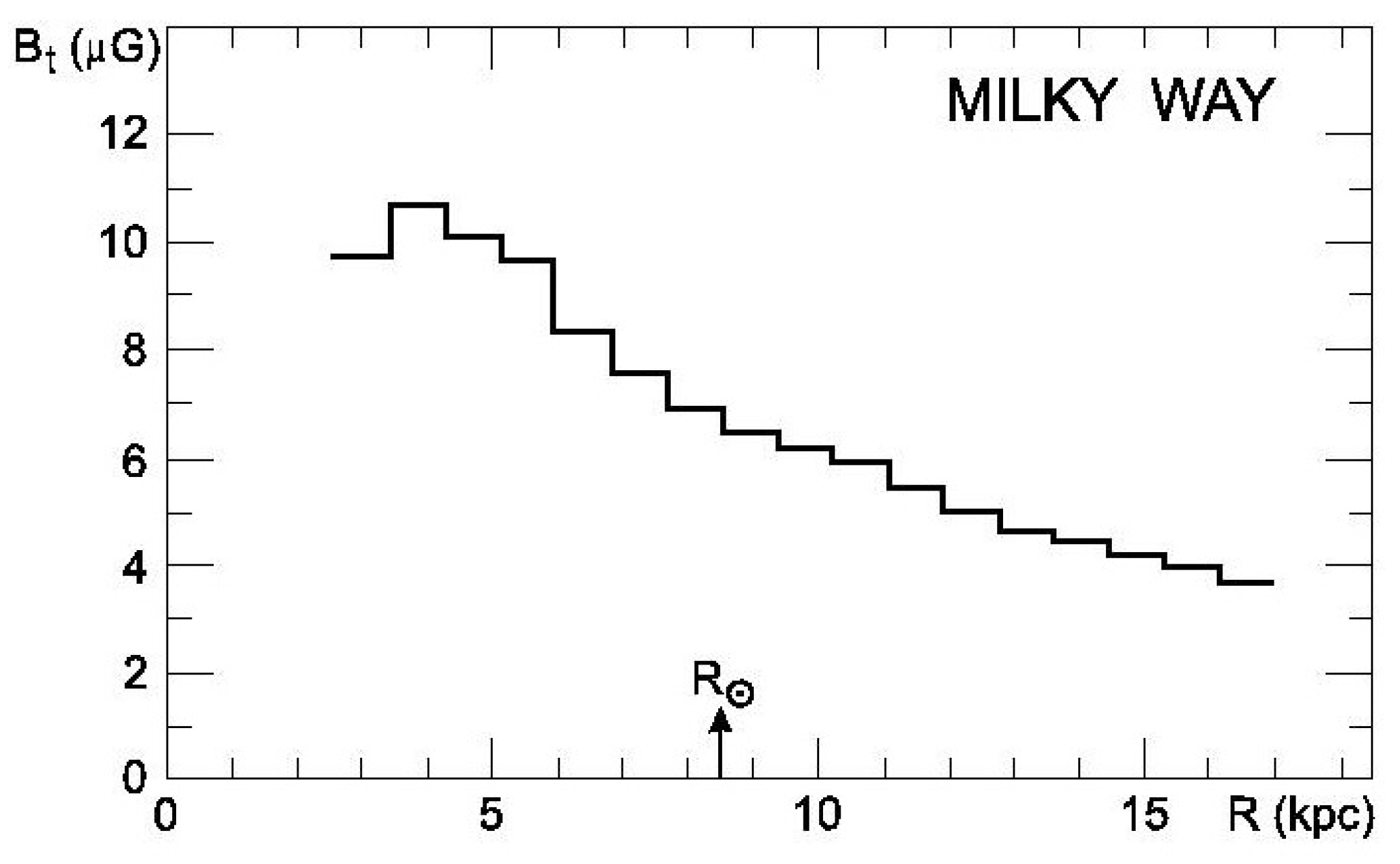
The average equipartition strength of the total fields derived from the total synchrotron intensity (using the classical estimate, scaled to $K=100$) for a sample of 146 late-type spiral galaxies is $B_{\mathrm{tot},\perp }=11\pm 4\mathsf{\mu }$G [35]. The sample of 74 spiral galaxies gave a similar value of $B_{\mathrm{tot}}=9\pm 2\mathsf{\mu }$G [37]. The total equipartition field strength in the Milky Way is about $10\mathsf{\mu }$G at a 5-kpc galactocentric radius with a decline to about $4\mathsf{\mu }$G at a 15-kpc radius (Figure 1).

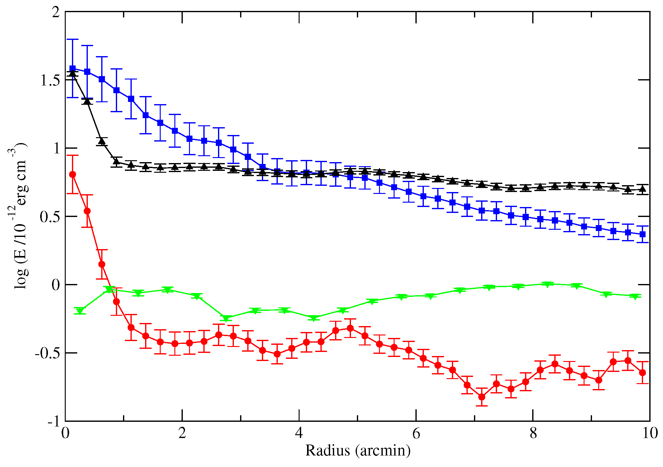
The equipartition estimates for several spiral galaxies [39,40] indicate that the magnetic energy density (dominated by the energy density of the small-scale field) is similar to the kinetic turbulent energy density (Figure 2), as expected for the operation of a turbulent dynamo, while the thermal energy density is about one order of magnitude smaller (low-$\beta$-plasma). A similar result was also obtained for the Milky Way in the solar neighbourhood [1].

The magnetic energy density in IC 342 seems to dominate at large radii (Figure 2), which can be explained with non-linear dynamo models [41] if the large-scale fields dominate out there, but this may also indicate that equipartition is no longer valid in the outer disk, e.g., due to fast cosmic-ray propagation.

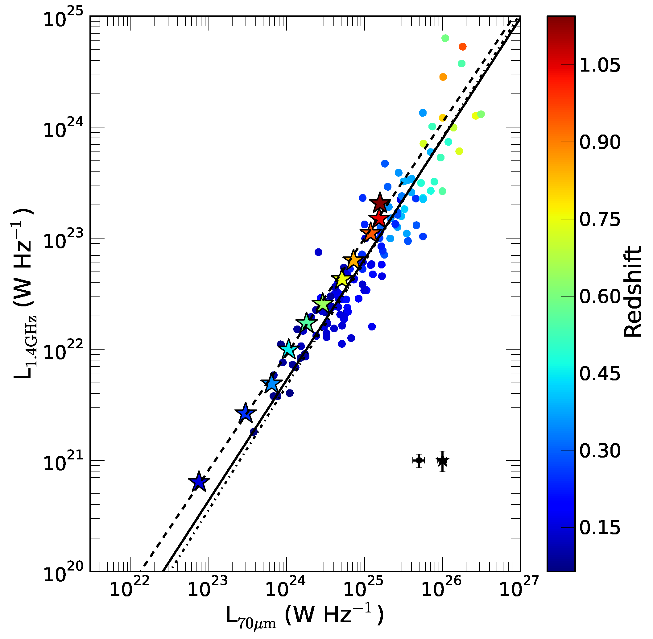
Another indication for the validity of the equipartition assumption at galaxy scale comes from the global correlation between the galaxy-integrated luminosity of the total radio continuum emission at frequencies of around 1 GHz, which is mostly of synchrotron origin, and the infrared (IR) luminosity of star-forming galaxies. This is one of the tightest correlations known in astronomy. The correlation extends over five orders of magnitude [42] and is slightly super-linear in log-log scale with an exponent of $1.09\pm 0.05$ [43] (Figure 3). The exponent of the non-thermal (synchrotron)-IR correlation must be steeper because the correlation between radio thermal and IR luminosities is linear [44] because UV photons ionize the gas and heat the warm dust. The exponent of the radio–IR correlation for thermal-corrected synchrotron luminosities is $1.33\pm 0.10$ [44]. The equipartition model [45] relates total (mostly turbulent) magnetic fields, cosmic rays, gas density and star formation and is able to explain the super-linear synchrotron-IR correlation.3

4.3. How Do Magnetic Field Strengths Derived from the Equipartition Assumption Compare with Those from Other Methods?

The Faraday rotation measure ($RM$) is a signature of the regular field $B_{\mathrm{reg},\Vert }$ along the line of sight and can be used to constrain the total field strength in galaxies. For example, $\left|RM\right|\simeq$100 rad/m${}^2$ in the magnetic arms of the spiral galaxy NGC 6946 yields $B_{\mathrm{reg}}\simeq 8\mathsf{\mu }$G for a typical electron density of $n_e\simeq 0.03$ cm${}^{-3}$, a pathlength of 1 kpc and an inclination of the galaxy’s disk of ${30}^{°}$ [47]. A degree of field order of $B_{\mathrm{reg}}/B_{\mathrm{tot}}\simeq 0.6$ follows from the observed degree of synchrotron polarization at high radio frequencies. As the contribution of anisotropic turbulent fields to the ordered field is probably small in the magnetic arms (located between the optical arms), $B_{\mathrm{reg}}\simeq B_{\mathrm{ord}}$. This gives $B_{\mathrm{tot}}\simeq 13\mathsf{\mu }$G, consistent with the equipartition estimate derived for the same regions.

Various measurements in the Milky Way confirm the equipartition estimate of the total field strength. From the dispersion of pulsar RMs, the galactic magnetic field was found to have a significant turbulent component with a mean strength of about $6\mathsf{\mu }$G [48]. The strength of the local regular field is about $2\mathsf{\mu }$G [49]. Zeeman splitting observations of low-density gas clouds (that have trapped the field from the diffuse ISM) yield field strengths of about $6\mathsf{\mu }$G, corrected for effects of the line-of-sight [50,51].

The Voyager 1 spacecraft reached interstellar space in 2012 and since then measured a constant total field strength of $4.8\pm 0.4\mathsf{\mu }$G [52]. The interstellar field is draped around the heliopause. A 3D magnetohydrodynamic (MHD) model of this interaction yielded a strength of the pristine local interstellar field of $2.9\pm 0.1\mathsf{\mu }$G [53]. This value is close to the strength of the local regular field.

Measurement of $B_{\mathrm{tot}}$ without the need for the equipartition assumption is possible if independent information about the cosmic-ray spectra is available. Cosmic rays can be measured directly in the solar neighbourhood where equipartition was found to be valid, and the magnetic field, cosmic ray and kinetic energies are roughly equal [1]. The density of CREs can be inferred from their X-ray emission by the inverse Compton (IC) effect, e.g., in galaxy clusters [54]. IC X-ray emission from star-forming galaxies has not yet been detected because other sources of X-ray emission are dominant. $\gamma$-rays generated by interactions of cosmic-ray protons with gas nuclei give information about the energy density of protons. Modelling the $\gamma$-ray and radio emissions allowed constraining the magnetic and cosmic-ray energy densities in the Milky Way and a few galaxies. Global equipartition is found to be valid in the Milky Way, M 31 and in the LMC [55].

From radio and $\gamma$-ray data in the Milky Way, a model of the radial variation of $B_{\mathrm{tot}}$ was constructed (Figure 6 in [56]), which agrees well with the equipartition estimates (Figure 1). More recent modelling yielded field strengths near the Sun of about 5 $\mathsf{\mu }$G of the isotropic turbulent field, about 2 $\mathsf{\mu }$G of the anisotropic turbulent field and about 2 $\mathsf{\mu }$G of the regular field [57], adding up (quadratically) to a total field strength of about 6 $\mathsf{\mu }$G.

4.4. Observational Indications for Deviations from the Equipartition Assumption

The total radio and IR intensities within galaxies are also highly correlated, but sub-linearly with exponents of $0.78\pm 0.02$ for M 31 and $0.46\pm 0.02$ for M 33, probably due to CRE propagation [58]. This indicates that equipartition between magnetic fields and cosmic rays is no longer valid at spatial scales below a few kpc. The exponent of the local correlation within 12 spiral galaxies varies between 0.3 and 0.8 [59], probably due to differences in the mean propagation length (which is defined as the product of the lifetime within the galaxy and the mean propagation speed) of CREs due to diffusion or advection. For a constant density of CREs, the exponent of the local radio synchrotron-IR correlation is smaller by a factor of $(1+\alpha )/(3+\alpha )\simeq 0.4–0.5$ compared to that of the global correlation for which equipartition holds, consistent with the observations. As the lifetime of cosmic-ray protons is longer than that of electrons, their mean propagation length is also larger, which may increase the spatial scale beyond which equipartition is valid.

The correlation analysis of the fluctuations in total radio intensity observed in the Milky Way and the nearby galaxy M 33 by [27] gave further evidence that equipartition does not hold at scales smaller than about 1 kpc. The equipartition field strength is probably underestimated in regions close to the CRE sources and overestimated in regions far away from the sources.

Modelling the radio and $\gamma$-ray data indicated that the global magnetic energy density is by a factor of several higher than the global cosmic-ray energy density in the central regions of the starburst galaxies M 82 and NGC 253 and even higher by several orders of magnitude in the ultraluminous infrared starburst galaxy Arp 220, where a field strength on the milligauss level was found [55]. It seems that the amount of deviation from equipartition increases with gas density, due to severe collisional energy losses of the cosmic-ray protons. Hence, the equipartition assumption heavily underestimates the magnetic field strength in dense starburst galaxies, which is of particular importance for the interpretation of galaxies in the early Universe.

The equipartition condition probably fails also in dwarf galaxies with a low star-formation rate (SFR) and hence a discontinuous supply of CRs [60]. Below $SFR\simeq 0.01$ M${}_{\mathrm{o}}$/year, radio synchrotron emission no longer traces the SFR, and the equipartition field strength is no longer correlated with SFR [61].

5. Testing of the Equipartition Assumption at Small Scales from Direct Numerical Simulations

Cosmic rays interact with magnetic fields in the ISM (further discussed in Section 5.1), and here, we model this interaction using test-particle (Section 5.2) and MHD (Section 5.3) simulations. The aim is to obtain the spatial distributions of cosmic rays and magnetic fields and then correlate them to test the energy equipartition argument.

5.1. Cosmic Ray–Magnetic Field Interaction

The Larmor radius r_L of a cosmic ray particle with a non-dimensional charge Z (charge of the particle divided by the proton or electron charge) and energy E propagating in a magnetic field of strength B is given by:

$$\begin{array}{cc}{r}_{\mathrm{L}}& \simeq 100\mathrm{pc}\frac{(E/{10}^8\mathrm{GeV})}{Z(B/1\mathsf{\mu }\mathrm{G})}.\end{array}$$

(5)

Low-energy cosmic ray particles, i.e., particles with Larmor radii less than the correlation length of the magnetic field, propagate diffusively within the galaxy. This is due to scattering by magnetic fluctuations with scales comparable to the cosmic ray Larmor radius [2,3,62]. The correlation length $l_b$ of small-scale magnetic fields in galaxies as suggested by small-scale dynamo simulations (Section 5.2, [63]), $l_b\simeq (1/3)l_0\approx 30$ pc, is less than the driving scale of the ISM turbulence, $l_0\approx 100$ pc. For an electron in the ISM magnetic field of around $5\mathsf{\mu }$G, using Equation (5), we find that the particles with $E\le {10}^8$ GeV have $r_{\mathrm{L}}<l_b$. Further, electrons with energy E in a magnetic field of strength B radiate mostly at the frequency ${\nu }_{\max }$, given by [64]:

$$\begin{array}{c}\hfill {\nu }_{\max }\simeq 16\mathrm{MHz}\frac{B}{1\mathsf{\mu }\mathrm{G}}{\left(\frac{E}{1\mathrm{GeV}}\right)}^2.\end{array}$$

(6)

Therefore, for radio frequencies in the range $150\mathrm{MHz}–1.5\mathrm{GHz}$ (wavelength $\approx 0.5–20\mathrm{cm}$), with a typical galactic magnetic field of around 5 $\mathsf{\mu }$G, the electron energy using Equation (6) is in the range of $1–10$ GeV. Thus, almost all of the synchrotron generating electrons are propagating diffusively in galaxy disks. The protons considered in the equipartition argument are those in the same energy range. The Larmor radius of a 5- GeV cosmic ray particle (proton or electron) in a $5\mathsf{\mu }$G magnetic field is ${10}^{-6}$ pc, which is much smaller than the correlation length of both the small-scale ($l_b<100$ pc) and the large-scale (few $\mathrm{kpc}$ in spiral galaxies) magnetic fields. The Larmor radius of heavier nuclei is even smaller. Thus, the particles are following the field, and it is important to consider the small-scale structure of the magnetic field for studying cosmic ray diffusion. This motivates us to consider cosmic rays as test-particles propagating in a random magnetic field generated by a non-linear small-scale dynamo (Section 5.2).

Cosmic rays via their interaction with magnetic fields also exert pressure on the thermal gas. This affects the gas velocity, which in turn affects the magnetic fields. The magnetic field further controls the cosmic ray propagation, and thus, it is important to consider the effect of the cosmic ray pressure. The energy density of cosmic rays in the solar neighbourhood $E_{\mathrm{cr}}$ estimated from the Voyager and Pioneer spacecraft data is approximately equal to $1.8\mathrm{eV}{\mathrm{cm}}^{-3}$ [65]. Then, the cosmic ray fluid pressure is given by:

$$\begin{array}{c}\hfill P_{\mathrm{cr}}=({\gamma }_{\mathrm{cr}}-1)E_{\mathrm{cr}},\end{array}$$

(7)

where ${\gamma }_{\mathrm{cr}}$ is the adiabatic index, which is equal to $4/3$ for cosmic rays since it is a relativistic fluid. For $E_{\mathrm{cr}}=1.8\mathrm{eV}{\mathrm{cm}}^{-3}$, using Equation (7), we obtain $P_{\mathrm{cr}}\simeq 4\times {10}^{-12}\mathrm{dyn}{\mathrm{cm}}^{-2}$. For an ISM magnetic field of strength $5\mathsf{\mu }$G, the magnetic field pressure is $P_{\mathrm{B}}=B^2/8\pi \simeq {10}^{-12}\mathrm{dyn}{\mathrm{cm}}^{-2}$. Thus, both the pressures are comparable, and the cosmic ray pressure significantly affects the ISM dynamics. We thus consider cosmic rays as a diffusive fluid in Section 5.3 to account for the pressure contribution. However, the pressure equality advocated here has average values and does not necessarily imply that cosmic rays and magnetic fields have the same pressure locally.

5.2. Cosmic Rays as Test-Particles

Cosmic rays can be treated as test-particles to study their diffusion in random magnetic fields, especially to understand how the cosmic ray diffusivity depends on the energy of the particle and properties of the magnetic fields [5,66,67,68,69]. In this work, to obtain random magnetic fields, we numerically solve the equations (Equations (8)–(10)) for the non-linear small-scale dynamo. For an isothermal gas with equation of state $p_{\mathrm{g}}=c_s^2\rho$, where $p_{\mathrm{g}}$ is the gas pressure, $c_s$ is the constant sound speed and $\rho$ is the gas density, we solve the equations for mass conservation (Equation (8)), magnetic induction (Equation (9)) and the Navier–Stokes equation (Equation (10)) in a periodic box of dimensionless size ${\left(2\pi \right)}^3$ with ${512}^3$ points using the Pencil code4. The governing equations are:

$$\begin{array}{c}\frac{\partial \rho }{\partial t}+\nabla ·\left(\rho \mathbf{u}\right)=0,\end{array}$$

(8)

$$\begin{array}{c}\frac{\partial \mathbf{b}}{\partial t}=\nabla \times (\mathbf{u}\times \mathbf{b})+\eta {\nabla }^2\mathbf{b},\end{array}$$

(9)

$$\begin{array}{c}\frac{\partial \mathbf{u}}{\partial t}+\mathbf{u}·\nabla \mathbf{u}=\frac{-\nabla p_{\mathrm{g}}}{\rho }+\frac{\mathbf{j}\times \mathbf{b}}{c\rho }+{\nu }_{\mathrm{kin}}\left({\nabla }^2\mathbf{u}+\frac{1}{3}\nabla \nabla ·\mathbf{u}+2\mathbf{S}·\nabla ln\rho \right)+\mathbf{F},\end{array}$$

(10)

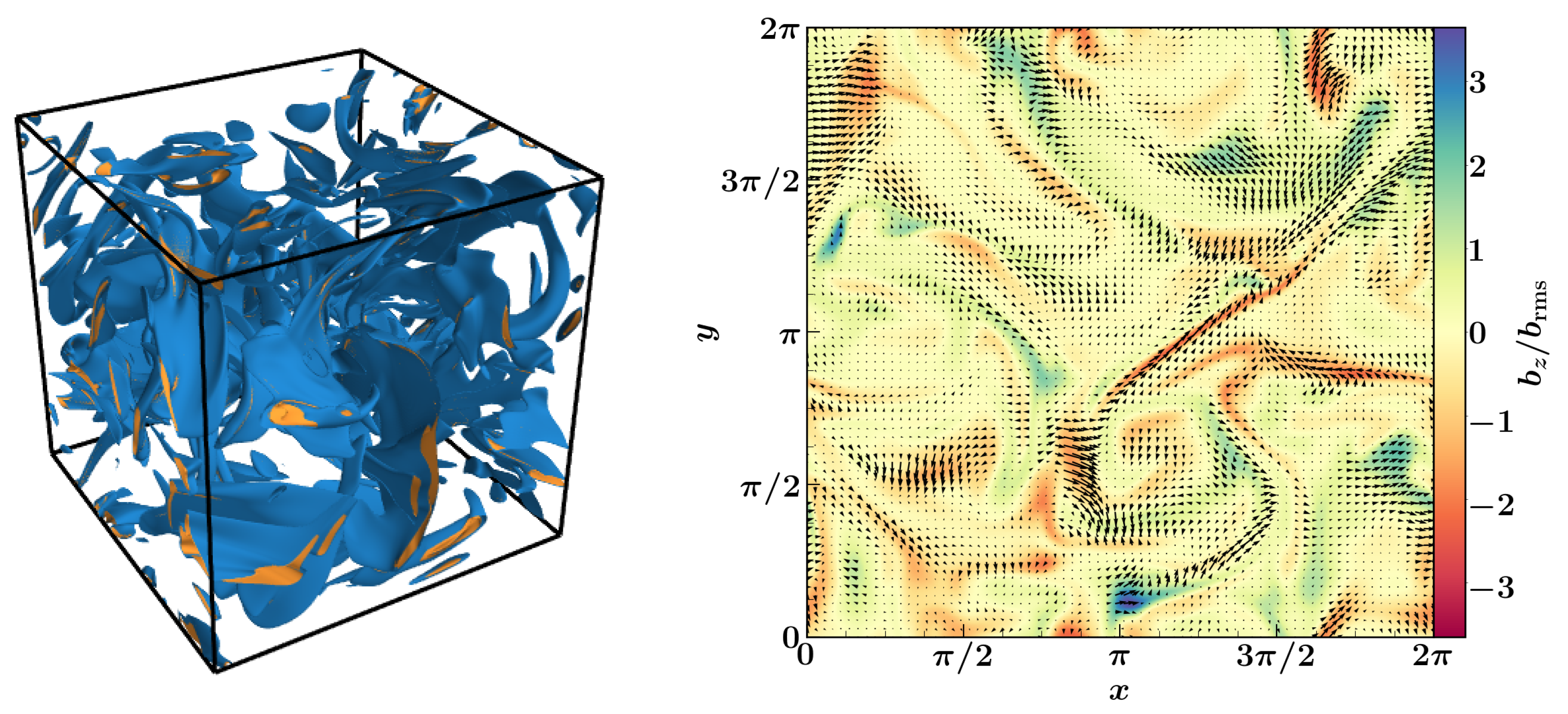
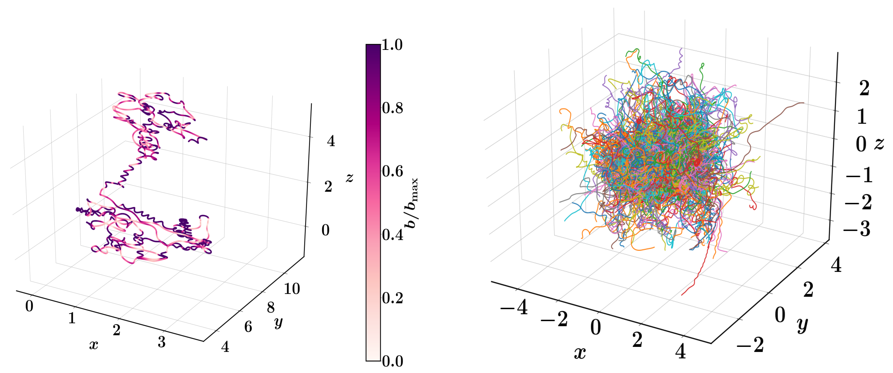
where $\mathbf{u}$ is the velocity, $\mathbf{b}$ is the magnetic field, $\eta$ is the magnetic diffusivity, $p_{\mathrm{g}}$ is the gas pressure, $\mathbf{j}$ is the current density, ${\nu }_{\mathrm{kin}}$ is the kinematic viscosity, $\mathbf{S}$ is the rate of strain tensor and $\mathbf{F}$ is the forcing function. The flow is driven by a forcing that is mirror-symmetric, nearly incompressible and $\delta$-correlated in time, equally at wavenumbers $k=2\pi /L$ and $k=2(2\pi /L)$, where L (here $L=2\pi$) is the size of the domain, in spectral space [70]. The average wavenumber, k_F, at which the flow is driven is approximately equal to $1.5(2\pi /L)$ and, thus, the numerical driving scale of turbulence $l_0$ is $2\pi /$k_F (physically equal to 100 pc). The amplitude of forcing is chosen to ensure that the flow remains subsonic. For simplicity, we choose ${\nu }_{\mathrm{kin}}=\eta$, which is chosen to be equal to ${10}^{22}{\mathrm{cm}}^2{\mathrm{s}}^{-1}$ (numerical simulations at the given resolution of $L/512$ resolve the viscous and resistive scales of that order). We initialized the box with zero velocity, uniform gas density and very weak seed Gaussian random magnetic field with the mean equal to zero. The magnetic field first grows exponentially, but then saturates due to the back-reaction by the Lorentz force. The correlation length of the saturated small-scale magnetic field $l_b$, calculated using the magnetic power spectrum, is approximately equal to $(1/3)l_0$ ($l_b/l_0$ for the saturated magnetic field does not vary much when the parameters ${\nu }_{\mathrm{kin}}$ and $\eta$ of the simulation are changed within a range [63]). Here, we present all quantities from the simulations in non-dimensional units. The magnetic field generated by the small-scale dynamo is spatially intermittent (random field with rare high peaks). Figure 4 shows the three-dimensional structure (left-hand panel) and a two-dimensional cut (right-hand panel) of the saturated magnetic field. The magnetic field is concentrated in magnetic structures of various shapes and sizes, mostly sheets and filaments [71]. We expect that a cosmic ray particle would propagate differently within a magnetic structure and between two such structures.

The trajectory of a cosmic ray particle is governed by the Lorentz force equation, given by:

$$\frac{{\mathrm{d}}^2\mathbf{r}}{{\mathrm{d}t}^2}=\frac{v}{r_{\mathrm{L}}}\frac{\mathrm{d}\mathbf{r}}{\mathrm{d}t}\times \frac{\mathbf{b}}{b_{\mathrm{rms}}},$$

(11)

where $\mathbf{r}\left(t\right)$ is the particle position at time t, v is the particle speed, $\mathbf{b}$ is the magnetic field and r_L is the Larmor radius of the particle defined with respect to the root mean square (rms) value of the magnetic field b_rms in the domain. r_L is a measure of the particle energy; in this work, we use the non-dimensional parameter $r_{\mathrm{L}}/l_0$. Since we are primarily interested in cosmic ray diffusion, we neglect any kind of acceleration of particles. We thus consider only a time-steady magnetic field (a single snap shot, which is shown in Figure 4). Furthermore, we do not consider particle energy losses, and thus, we model only the proton component of cosmic rays for which the energy loss within the confinement time of cosmic rays in galaxies (≈${10}^7$ year) is negligible. The left-hand panel of Figure 5 shows the trajectory of a single particle for $r_{\mathrm{L}}/l_0=0.02$. The particle gyrates around the magnetic field in structures where the field is strong and is scattered in the region where the field is weak. Over large time and length scales for an ensemble of particles (right-hand panel of Figure 5), this gives rise to diffusion. We solve Equation (11) for an ensemble of particles that are placed randomly within the domain with the same speed, but random velocity directions. We confirm that the particles diffuse by calculating the time-steady diffusion coefficient [5,72]. Once the diffusion sets in, we calculate the coordinates of each particle modulo the length of the box ($2\pi$), divide the entire domain into ${512}^3$ smaller cubes and count the number of particles in each cube to obtain the particle number density as a function of position and time. Then, we average this distribution over a long time to obtain the time independent cosmic ray distribution $n_{\mathrm{cr}}$.

The cross-correlation coefficient between cosmic rays and magnetic fields is calculated using:

$$C(n_{\mathrm{cr}},b^2)=\frac{\langle n_{\mathrm{cr}}{b}^2\rangle -\langle n_{\mathrm{cr}}\rangle \langle b^2\rangle }{{\sigma }_{n_{\mathrm{cr}}}{\sigma }_{b^2}},$$

(12)

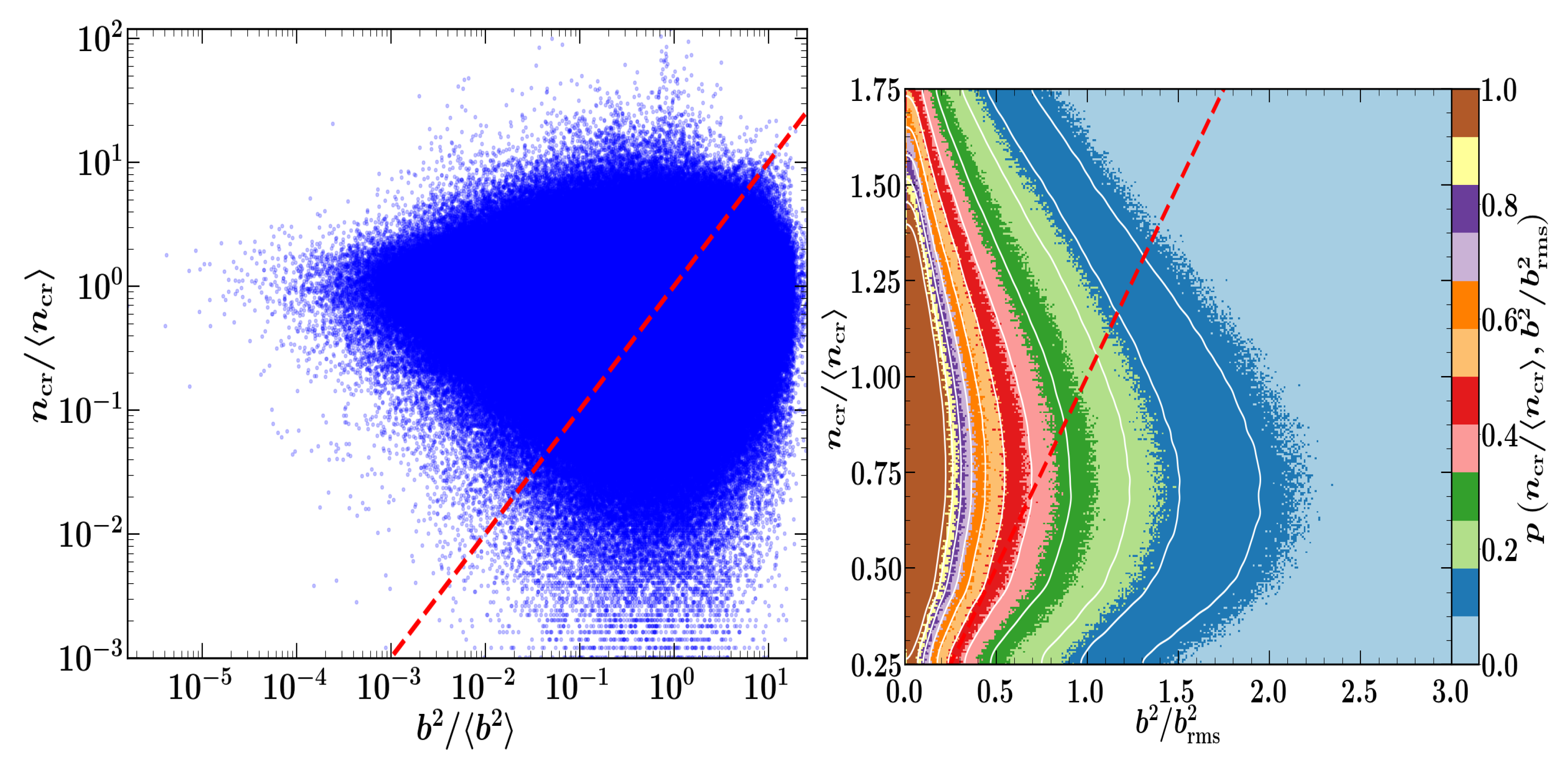
where $\langle \cdots \rangle$ and $\sigma$ implies the average and standard deviation of quantities over the entire domain. The cross-correlation coefficient C is approximately equal to zero for various particle energies ($r_{\mathrm{L}}/l_0$). This confirms that the two quantities are uncorrelated at scales less than the driving scale of the turbulence $l_0$ (here, approximately the size of the box). The correlation remains close to zero even when a regular large-scale field and pitch angle scattering due to small-scale magnetic fluctuations (which are not resolved in the nonlinear small-scale dynamo simulation [72]) are included. The left-hand panel of Figure 6 shows a scatter plot of the cosmic ray number density and magnetic field energy density, which further confirms the lack of correlation between two quantities. The right-hand panel of Figure 6 shows the joint probability distribution function (PDF) of the cosmic ray number density and magnetic field energy density where the majority of points lie. This too demonstrates that the most points lie away from the red dashed line, which shows a one-to-one correlation between two quantities.

The left-hand panel of Figure 6 shows cosmic ray number densities that are significantly higher and lower than the mean value. This suggests an inhomogeneous cosmic ray distribution. Due to a finite number of particles, the initial distribution in such simulations is not completely isotropic and homogeneous, and this makes the final distribution inhomogeneous5. These localized areas of high cosmic ray density are the regions with magnetic bottle traps, and this is confirmed in numerical simulations by looking at particle trajectories in the vicinity of a trap [72]. The presence of such traps enhances cosmic ray density at certain locations (or reduces at others), but those are not necessarily the strong magnetic field (or the weak magnetic field) regions. Furthermore, trapping might change the proton to electron ratio K. Both protons and electrons would spend more time in magnetic traps (as compared to non-trapping regions), but electrons, since they lose energy, get slower and are trapped for a longer time as compared to protons. This would change the factor K (also see Point (2) in Section 3.2). Moreover, in such a situation, K would not be a fixed constant and would depend on the location and energy of the particle. Having said that, such traps are only of relevance at small scales (less than the correlation length of the small-scale magnetic field, $l_b\simeq (1/3)l_0\approx 30$ pc) and may not affect the conclusions at larger $\mathrm{kpc}$ scales.

5.3. Cosmic Rays as a Diffusive Fluid in MHD Turbulence

To consider the effect of the cosmic ray pressure, we solved the MHD equations using a two-fluid model: gas with adiabatic index ${\gamma }_{\mathrm{g}}=5/3$ (a non-relativistic fluid) and cosmic rays with adiabatic index ${\gamma }_{\mathrm{cr}}=4/3$ (a relativistic fluid). For an isothermal gas with equation of state, $p_{\mathrm{g}}=c_s^2\rho$, where $p_{\mathrm{g}}$ is the gas pressure, $c_s$ is the constant sound speed and $\rho$ is the gas density, we solve equations for mass conservation (Equation (8)), magnetic induction (Equation (9)), Navier–Stokes equation (Equation (10)), but now also including the cosmic ray pressure (i.e., the first term in the right-hand side is modified to $-\nabla (p_{\mathrm{g}}+p_{\mathrm{cr}})/\rho$), and cosmic ray advection-diffusion (Equation (13) and Equation (14)) in a box of dimensionless size ${\left(2\pi \right)}^3$ (periodic boundary condition for y and z, stress-free normal field boundary condition with energy density of cosmic rays $e_{\mathrm{cr}}=0$ at boundaries $x=0$ and $x=2\pi$) with ${256}^3$ points. The forcing function and its parameters for a turbulent driving in the Navier–Stokes equation is the same as described in Section 5.2. The cosmic ray advection-diffusion equation is:

$$\begin{array}{c}\hfill \frac{\partial e_{\mathrm{cr}}}{\partial t}+\nabla ·\left(e_{\mathrm{cr}}\mathbf{u}\right)+p_{\mathrm{cr}}\nabla ·u=-\nabla ·{\mathbf{F}}_{\mathrm{cr}}+Q_{\mathrm{cr}},\end{array}$$

(13)

where $e_{\mathrm{cr}}$ is the cosmic ray energy density, $p_{\mathrm{cr}}=({\gamma }_{\mathrm{cr}}-1)e_{\mathrm{cr}}$ is the cosmic ray pressure and $Q_{\mathrm{cr}}$ is the cosmic ray energy source by which cosmic rays are injected uniformly throughout the volume at a constant rate (note that the cosmic rays are lost via the boundaries in the x direction). The cosmic ray flux ${\mathbf{F}}_{\mathrm{cr}}$ is defined via the equation:

$$\begin{array}{c}\hfill \tau \frac{\partial F_{\mathrm{cr}i}}{\partial t}=-{\kappa }_{ij}{\nabla }_j{e}_{\mathrm{cr}}-F_{\mathrm{cr}i},\end{array}$$

(14)

where $\tau$ is the cosmic ray flux correlation time and ${\kappa }_{ij}$ is the diffusion coefficient. ${\kappa }_{ij}={\kappa }_{\perp }{\delta }_{ij}+({\kappa }_{\Vert }-{\kappa }_{\perp }){\widehat{\mathbf{b}}}_i{\widehat{\mathbf{b}}}_j$ is written in terms of the parallel ${\kappa }_{\Vert }$ and perpendicular ${\kappa }_{\perp }$ diffusion coefficients (${\widehat{\mathbf{b}}}_i$ is the unit vector along the i-axis). Here, we solve the telegraph equation (Equation (14)) to study cosmic ray diffusion instead of the usual diffusion equation [73,74].

We solve these equations using the Pencil code [73] for parameters given in

Table 1. Non-dimensional parameters used to solve the magnetohydrodynamic (MHD) and cosmic ray fluid equations and their corresponding ISM values.

Parameter	Numerical Value	ISM Value
${\gamma }_{\mathrm{g}}$	$5/3$	$5/3$
${\gamma }_{\mathrm{cr}}$	$4/3$	$4/3$
kF	1 and 2	100 pc and 50 pc
${\nu }_{\mathrm{kin}}$	$2\times {10}^{-3}$	$2\times {10}^{23}{\mathrm{cm}}^2{\mathrm{s}}^{-1}$
$\eta$	$1\times {10}^{-3}$	$1\times {10}^{23}{\mathrm{cm}}^2{\mathrm{s}}^{-1}$
${\kappa }_{\Vert }$	$3\times {10}^{-1}$	$3\times {10}^{25}{\mathrm{cm}}^2{\mathrm{s}}^{-1}$
${\kappa }_{\perp }$	0	0
$\tau$	$3\times {10}^{-1}$	$0.3\mathrm{My}$
$Q_{\mathrm{cr}}$	$0.001,0.005,0.01$	$(0.001,0.005,0.01)\times {10}^{-26}\mathrm{erg}{\mathrm{cm}}^{-3}{\mathrm{s}}^{-1}$

6. All velocities are in units of the sound speed $c_s$; densities are in units of the initial gas density ${\rho }_0$; lengths are in units of the box size $L=2\pi$ (so that the smallest wavenumber is $k_1=2\pi /L$); time is in units of the eddy turn over time $t_0=1/u_{\mathrm{rms}}$k_F; the magnetic field in units of ${\left(4\pi {\rho }_0{c}_s^2\right)}^{1/2}$; and all the diffusivities are in units of $c_s/k_1$. All other units can be derived from these basic units. The unit of the cosmic ray source term $Q_{\mathrm{cr}}$ is ${\rho }_0{c}_s^3{k}_1$. We selected ${\kappa }_{\perp }=0$ for simplicity. The value of $\tau$ was chosen such that the maximum speed for signal propagation is of the order of ${({\kappa }_{\Vert }/\tau )}^{1/2}$. This was done to capture the initial non-diffusive or ballistic phase of cosmic rays in random magnetic fields [74].

There are a few differences between the ISM parameters in our simulations (Table 1) and those estimated for the ISM from observations or existing models. First, it is inferred from the observed radio polarization gradients that the ISM turbulence is quite compressive with a Mach number around one [77], while our simulations are at a very low Mach number (∼0.1). Second, using kinetic theory arguments, the ratio of resistivity to viscosity in the ISM can be estimated to be of the order of ${10}^{11}$ [12]; however, for our simulations, it was of the order of one. Furthermore, the cosmic ray diffusivity was also chosen to be smaller than the reported value of ${10}^{28}{\mathrm{cm}}^2{\mathrm{s}}^{-1}$ [75], a number obtained from the abundance ratio of the radioactive and stable isotopes of Beryllium in cosmic rays. All diffusive effects (viscosity, resistivity and cosmic ray diffusivity) are much lower than those estimated in the ISM due to the limited numerical resolution. These estimated parameters might be important for comparing simulations with the observations, but do not affect the physics of cosmic ray–magnetic field interaction (additional pressure contribution due to cosmic rays), which we aim to capture in these numerical experiments.

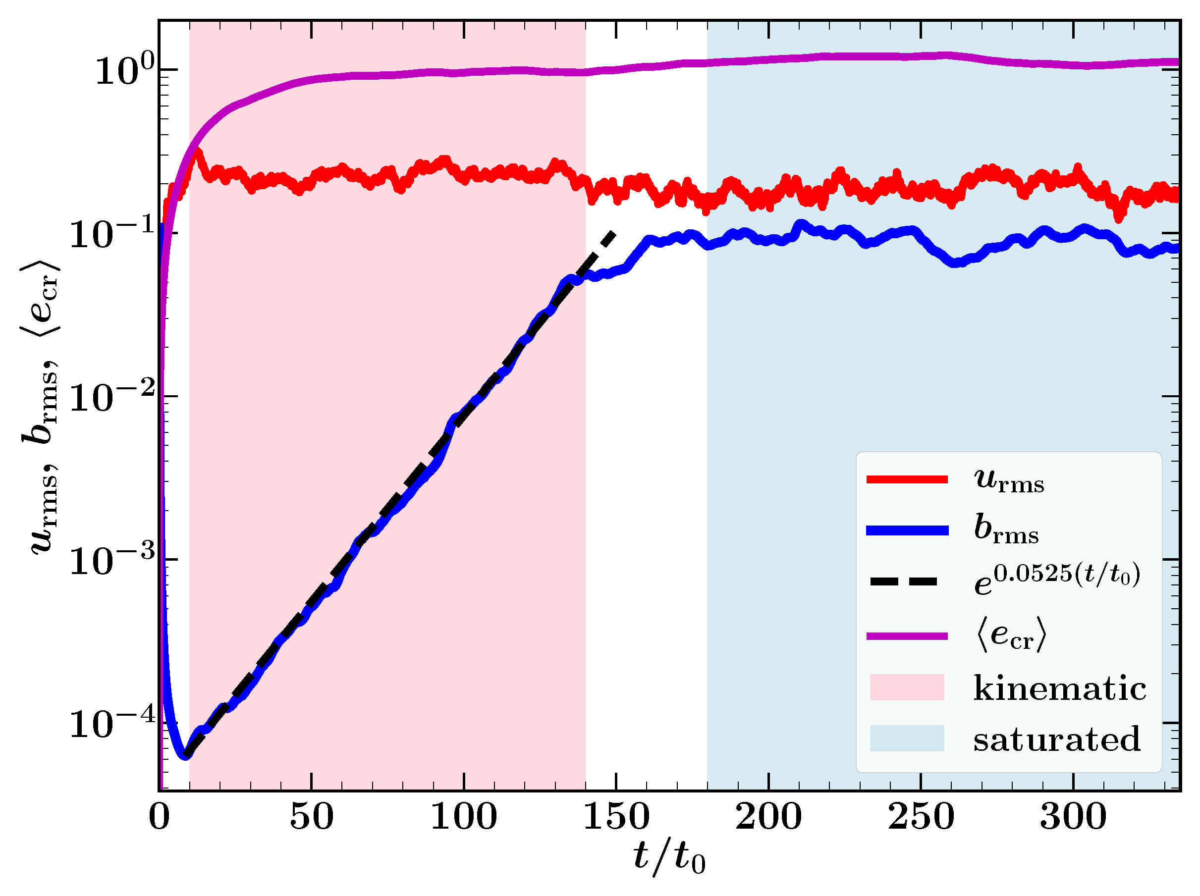
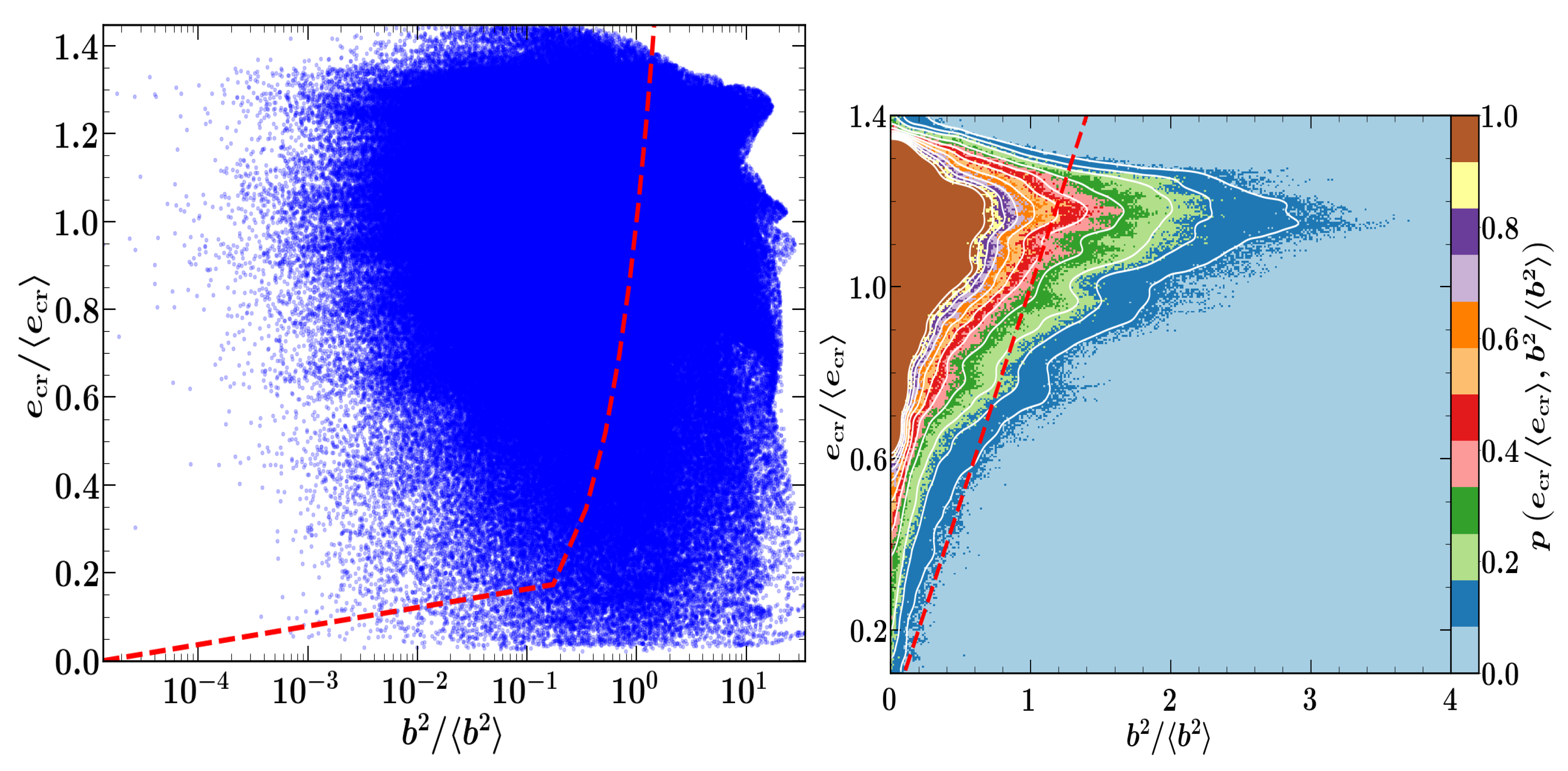
We chose three different values for the cosmic ray source term $Q_{\mathrm{cr}}$ to have the following three different cases in the saturated stage: $\langle e_{\mathrm{cr}}\rangle <b_{\mathrm{rms}}^2,\langle e_{\mathrm{cr}}\rangle \approx b_{\mathrm{rms}}^2,\langle e_{\mathrm{cr}}\rangle >b_{\mathrm{rms}}^2$. A uniform gas density and a weak (in the rms sense) Gaussian random magnetic field with zero mean was initialized within the numerical domain. The velocity and cosmic ray energy density were both initialized to zero, and with time, they both become non-zero due to continuous forcing $\mathbf{F}$ in the Navier–Stokes equation (Equation (10)) and the cosmic ray source term $Q_{\mathrm{cr}}$ in the advection-diffusion equation (Equation (13)), respectively. Figure 7 shows the evolution of the root mean square (rms) velocity field, rms magnetic field and mean cosmic ray energy density. The magnetic field first decays until it transforms into a growing eigenfunction of the induction equation7, and then, it increases exponentially (referred to as the kinematic stage). Finally, the magnetic field becomes strong enough, and the Lorentz force reacts back on the velocity flow saturating the magnetic field (referred to as the saturated stage). For all three cases, we find that the cross-correlation between cosmic rays and magnetic fields (using Equation (12)) is very close to zero. Thus, even after including the effect of cosmic ray pressure on the thermal gas, the cosmic rays and magnetic fields are not correlated at the scales less than the driving scale of the turbulence ($l_0\simeq 100$ pc or, equivalently, the numerical domain size in simulations). The left-hand panel of Figure 8 shows the scatter plot of the cosmic ray and magnetic field energy densities over the entire domain for the case where $\langle e_{\mathrm{cr}}\rangle \approx \langle b^2\rangle$ in the saturated state. The form of the plot confirms that the two quantities are not correlated. Furthermore, the right-hand panel of Figure 8 shows the joint PDF between the two quantities for most points in the domain, which also shows a lack of correlation. Thus, even when both energies are equal over the scale of the domain (by construction here), they are not correlated locally, so that equipartition is not valid.

6. Conclusions, Discussion and Future Directions of Research

Synchrotron emission depends on two quantities: cosmic ray electron number density and magnetic fields, so that assuming a relation between two quantities provides information about magnetic fields from synchrotron observations in star-forming galaxies. Thus, the energy equipartition argument is a convenient assumption. However, it is not a physical law, and thus, it is important to test its validity. After describing the method and theoretical arguments to expect the energy equipartition in star-forming galaxies, this paper discusses its validity using observational results and numerical simulations.

There is convincing observational evidence that equipartition between the energy densities of total magnetic fields and total cosmic rays is valid in normal star-forming galaxies, globally, as well as locally at spatial scales larger than a certain threshold, possibly related to the mean propagation length of the cosmic rays of ≈1 kpc and can be safely used to estimate the total magnetic fields’ strength from the total synchrotron intensity. If the synchrotron-radiating CREs have lost a significant fraction of their energy, e.g., in dense regions of the interstellar medium or in galaxy halos, a corrected proton/electron ratio has to be used in the formula. Equipartition is not valid in starburst regions or in ultraluminous infrared galaxies. The equipartition condition may also fail in dwarf galaxies [61].

Future observations should investigate the threshold scale between the regime of equipartition and non-equipartition and its dependence on galaxy properties. The exponent of the radio-infrared correlation within galaxies should be measured at different scales, to fix the transition from super-linear to sub-linear. As the threshold scale is possibly related to the average propagation length of CR(E)s, a spatial resolution down to about 100 pc for a sample of galaxies is needed, which calls for high angular resolution (1–2 arcsec) in galaxies at 10–20-Mpc distances. Present-day radio telescopes allow us to observe only the nearest and brightest galaxies with such a resolution. Increasing the galaxy sample will have to wait for the Square Kilometre Array (SKA) [78].

More and better tests of equipartition with the help of $\gamma$-rays require sensitive observations of many nearby galaxies with different star-formation rates. ESA’s e-ASTROGAMsatellite project plan is promising [79].

Using both the test-particle simulations in realistic (small-scale dynamo generated) random magnetic fields and the MHD simulations, we showed that the cosmic ray energy density (or equivalently number density) is not correlated to the magnetic field energy density at scales smaller than the driving scale of the turbulence (≈100 pc in spiral galaxies). This scale can be regarded as the lower limit for the scale beyond which equipartition is valid. In test-particle simulations, the particles sample the small-scale structure of random magnetic fields, which is an important ingredient (magnetic power at smaller scale) to justify energy equipartition assumption via the confinement argument (second argument in Section 2). In MHD simulations, the effect of cosmic ray pressure is also included. This is considered to test the local pressure equality between cosmic rays and magnetic fields. The results from both kinds of simulations (Figure 6 and Figure 8) suggest a lack of energy equipartition at smaller scales. This is in agreement with the observational results (Section 4.2 and Section 4.4). However, our simulations do not exclude that energy equipartition is valid at larger scales.

Cosmic rays in our MHD simulations only exert pressure on the thermal gas, but it can also heat up the medium. Cosmic rays scatter off waves excited by the streaming instability [2,3,80] and then stream at the Alfvén speed down their pressure gradient. The excited waves are damped, and their energy is deposited in the ISM, which heats it up. This could be modelled in our numerical simulations (a stable numerical scheme for the cosmic ray streaming was discussed in [81,82]). The cosmic ray streaming is particularly important for the launching of galactic winds [83,84] and the Parker instability [85]. Another extension of the numerical work would be to include cosmic rays in comparatively larger scale multiphase ISM simulations (domain size of a few $\mathrm{kpc}$) where the turbulence is driven by supernova explosions [86,87,88]. The cosmic rays would then accelerate in supernova shocks and diffuse away from their sources. One might recover equipartition at large scales in such studies.

References

- Boulares, A.; Cox, D.P. Galactic Hydrostatic Equilibrium with Magnetic Tension and Cosmic-Ray Diffusion. Astrophys. J. 1990, 365, 544. [Google Scholar] [CrossRef]
- Kulsrud, R.; Pearce, W.P. The Effect of Wave-Particle Interactions on the Propagation of Cosmic Rays. Astrophys. J. 1969, 156, 445. [Google Scholar] [CrossRef]
- Wentzel, D.G. Cosmic-ray propagation in the Galaxy—Collective effects. Annu. Rev. Astron. Astrophys. 1974, 12, 71–96. [Google Scholar] [CrossRef]
- Zweibel, E.G. The microphysics and macrophysics of cosmic raysa. Phys. Plasmas 2013, 20, 055501. [Google Scholar] [CrossRef]
- Shukurov, A.; Snodin, A.P.; Seta, A.; Bushby, P.J.; Wood, T.S. Cosmic Rays in Intermittent Magnetic Fields. Astrophys. J. Lett. 2017, 839, L16. [Google Scholar] [CrossRef]
- Birnboim, Y.; Balberg, S.; Teyssier, R. Galaxy evolution: Modelling the role of non-thermal pressure in the interstellar medium. Month. Not. R. Astron. Soc. 2015, 447, 3678–3692. [Google Scholar] [CrossRef]
- Krumholz, M.R.; Federrath, C. The Role of Magnetic Fields in Setting the Star Formation Rate and the Initial Mass Function. arXiv 2019, arXiv:1902.02557. [Google Scholar] [CrossRef]
- Bendre, A.; Gressel, O.; Elstner, D. Dynamo saturation in direct simulations of the multi-phase turbulent interstellar medium. Astron. Nachr. 2015, 336, 991. [Google Scholar] [CrossRef]
- Shukurov, A.; Evirgen, C.C.; Fletcher, A.; Bushby, P.J.; Gent, F.A. Magnetic field effects on the ISM structure and galactic outflows. arXiv 2018, arXiv:1810.01202. [Google Scholar]
- Klein, U.; Fletcher, A. Galactic and Intergalactic Magnetic Fields; Springer Praxis Books, Springer International Publishing: Heidelberg, Germany, 2015. [Google Scholar]
- Beck, R.; Brandenburg, A.; Moss, D.; Shukurov, A.; Sokoloff, D. Galactic Magnetism: Recent Developments and Perspectives. Annu. Rev. Astron. Astrophys. 1996, 34, 155–206. [Google Scholar] [CrossRef]
- Brandenburg, A.; Subramanian, K. Astrophysical magnetic fields and nonlinear dynamo theory. Phys. Rep. 2005, 417, 1–209. [Google Scholar] [CrossRef]
- Minter, A.H.; Spangler, S.R. Observation of Turbulent Fluctuations in the Interstellar Plasma Density and Magnetic Field on Spatial Scales of 0.01 to 100 Parsecs. Astrophys. J. 1996, 458, 194. [Google Scholar] [CrossRef]
- Haverkorn, M.; Brown, J.C.; Gaensler, B.M.; McClure-Griffiths, N.M. The Outer Scale of Turbulence in the Magnetoionized Galactic Interstellar Medium. Astrophys. J. 2008, 680, 362–370. [Google Scholar] [CrossRef]
- Iacobelli, M.; Haverkorn, M.; Orrú, E.; Pizzo, R.F.; Anderson, J.; Beck, R.; Bell, M.R.; Bonafede, A.; Chyzy, K.; Dettmar, R.J.; et al. Studying Galactic interstellar turbulence through fluctuations in synchrotron emission. First LOFAR Galactic foreground detection. Astron. Astrophys. 2013, 558, A72. [Google Scholar] [CrossRef]
- Ohno, H.; Shibata, S. The random magnetic field in the Galaxy. Month. Not. R. Astron. Soc. 1993, 262, 953–962. [Google Scholar] [CrossRef]
- Gaensler, B.M.; Haverkorn, M.; Staveley-Smith, L.; Dickey, J.M.; McClure-Griffiths, N.M.; Dickel, J.R.; Wolleben, M. The Magnetic Field of the Large Magellanic Cloud Revealed Through Faraday Rotation. Science 2005, 307, 1610–1612. [Google Scholar] [CrossRef]
- Fletcher, A.; Beck, R.; Shukurov, A.; Berkhuijsen, E.M.; Horellou, C. Magnetic fields and spiral arms in the galaxy M51. Month. Not. R. Astron. Soc. 2011, 412, 2396–2416. [Google Scholar] [CrossRef]
- Houde, M.; Fletcher, A.; Beck, R.; Hildebrand, R.H.; Vaillancourt, J.E.; Stil, J.M. Characterizing Magnetized Turbulence in M51. Astrophys. J. 2013, 766, 49. [Google Scholar] [CrossRef]
- Longair, M.S. High Energy Astrophysics. Volume 2. Stars, the Galaxy and the Interstellar Medium; Cambridge University Press: Cambridge, UK, 1994. [Google Scholar]
- Bell, A.R. The acceleration of cosmic rays in shock fronts. I. Month. Not. R. Astron. Soc. 1978, 182, 147–156. [Google Scholar] [CrossRef]
- Bell, A.R. The acceleration of cosmic rays in shock fronts. II. Month. Not. R. Astron. Soc. 1978, 182, 443–455. [Google Scholar] [CrossRef]
- Blandford, R.D.; Ostriker, J.P. Particle acceleration by astrophysical shocks. Astrophys. J. Lett. 1978, 221, L29–L32. [Google Scholar] [CrossRef]
- Drury, L.O. An introduction to the theory of diffusive shock acceleration of energetic particles in tenuous plasmas. Rep. Prog. Phys. 1983, 46, 973. [Google Scholar] [CrossRef]
- Burbidge, G.R. On Synchrotron Radiation from Messier 87. Astrophys. J. 1956, 124, 416. [Google Scholar] [CrossRef]
- Stepanov, R.; Fletcher, A.; Shukurov, A.; Beck, R.; La Porta, L.; Tabatabaei, F.S. Relative distributions of cosmic ray electrons and magnetic fields in the ISM. In Cosmic Magnetic Fields: From Planets, to Stars and Galaxies; Cambridge University Press: Cambridge, UK, 2009. [Google Scholar]
- Stepanov, R.; Shukurov, A.; Fletcher, A.; Beck, R.; La Porta, L.; Tabatabaei, F. An observational test for correlations between cosmic rays and magnetic fields. Month. Not. R. Astron. Soc. 2014, 437, 2201–2216. [Google Scholar] [CrossRef]
- Pohl, M. On the predictive power of the minimum energy condition. I—Isotropic steady-state configurations. Astron. Astrophys. 1993, 270, 91–101. [Google Scholar]
- Arbutina, B.; Urošević, D.; Andjelić, M.M.; Pavlović, M.Z.; Vukotić, B. Modified Equipartition Calculation for Supernova Remnants. Astrophys. J. 2012, 746, 79. [Google Scholar] [CrossRef]
- Caprioli, D. Understanding hadronic gamma-ray emission from supernova remnants. J. Cosmol. Astropart. Phys. 2011, 5, 026. [Google Scholar] [CrossRef]
- Morlino, G.; Caprioli, D. Strong evidence for hadron acceleration in Tycho’s supernova remnant. Astron. Astrophys. 2012, 538, A81. [Google Scholar] [CrossRef]
- Strong, A.W.; Moskalenko, I.V.; Reimer, O. Diffuse Galactic Continuum Gamma Rays: A Model Compatible with EGRET Data and Cosmic-Ray Measurements. Astrophys. J. 2004, 613, 962–976. [Google Scholar] [CrossRef]
- Picozza, P.; Marcelli, L.; Adriani, O.; Barbarino, G.C.; Bazilevskaya, G.A.; Bellotti, R.; Boezio, M.; Bogomolov, E.A.; Bongi, M.; Bonvicini, V.; et al. Cosmic Ray Study with the PAMELA Experiment. J. Phys. Conf. Ser. 2013, 409, 012003. [Google Scholar] [CrossRef]
- Beck, R.; Krause, M. Revised equipartition and minimum energy formula for magnetic field strength estimates from radio synchrotron observations. Astron. Nachr. 2005, 326, 414–427. [Google Scholar] [CrossRef]
- Fitt, A.J.; Alexander, P. Magnetic fields in late-type galaxies. Month. Not. R. Astron. Soc. 1993, 261, 445–452. [Google Scholar] [CrossRef]
- Lacki, B.C.; Beck, R. The equipartition magnetic field formula in starburst galaxies: Accounting for pionic secondaries and strong energy losses. Month. Not. R. Astron. Soc. 2013, 430, 3171–3186. [Google Scholar] [CrossRef]
- Niklas, S. Eigenschaften von Spiralgalaxien im Hochfrequenten Radiokontinuum. Ph.D. Thesis, University of Bonn, Bonn, Germany, 1995. [Google Scholar]
- Beuermann, K.; Kanbach, G.; Berkhuijsen, E.M. Radio structure of the Galaxy—Thick disk and thin disk at 408 MHz. Astron. Astrophys. 1985, 153, 17–34. [Google Scholar]
- Beck, R. Magnetic fields in the nearby spiral galaxy IC 342: A multi-frequency radio polarization study. Astron. Astrophys. 2015, 578, A93. [Google Scholar] [CrossRef]
- Basu, A.; Roy, S. Magnetic fields in nearby normal galaxies: Energy equipartition. Month. Not. R. Astron. Soc. 2013, 433, 1675–1686. [Google Scholar] [CrossRef]
- Chamandy, L.; Singh, N.K. Non-linear galactic dynamos and the magnetic Rädler effect. Month. Not. R. Astron. Soc. 2018, 481, 1300–1319. [Google Scholar] [CrossRef]
- Bell, E.F. Estimating Star Formation Rates from Infrared and Radio Luminosities: The Origin of the Radio-Infrared Correlation. Astrophys. J. 2003, 586, 794–813. [Google Scholar] [CrossRef]
- Basu, A.; Wadadekar, Y.; Beelen, A.; Singh, V.; Archana, K.N.; Sirothia, S.; Ishwara-Chandra, C.H. Radio-Far-infrared Correlation in “Blue Cloud” Galaxies with 0 < z < 1.2. Astrophys. J. 2015, 803, 51. [Google Scholar] [CrossRef]
- Price, R.; Duric, N. New results on the radio-far-infrared relation for galaxies. Astrophys. J. 1992, 401, 81–86. [Google Scholar] [CrossRef]
- Niklas, S.; Beck, R. A new approach to the radio-far infrared correlation for non-calorimeter galaxies. Astron. Astrophys. 1997, 320, 54–64. [Google Scholar]
- Hoernes, P.; Berkhuijsen, E.M.; Xu, C. Radio-FIR correlations within M 31. Astron. Astrophys. 1998, 334, 57–70. [Google Scholar]
- Beck, R. Magnetism in the spiral galaxy NGC 6946: Magnetic arms, depolarization rings, dynamo modes, and helical fields. Astron. Astrophys. 2007, 470, 539–556. [Google Scholar] [CrossRef]
- Han, J.L.; Ferriere, K.; Manchester, R.N. The Spatial Energy Spectrum of Magnetic Fields in Our Galaxy. Astrophys. J. 2004, 610, 820–826. [Google Scholar] [CrossRef]
- Han, J.L.; Manchester, R.N.; Lyne, A.G.; Qiao, G.J.; van Straten, W. Pulsar Rotation Measures and the Large-Scale Structure of the Galactic Magnetic Field. Astrophys. J. 2006, 642, 868–881. [Google Scholar] [CrossRef]
- Crutcher, R.M.; Wandelt, B.; Heiles, C.; Falgarone, E.; Troland, T.H. Magnetic Fields in Interstellar Clouds from Zeeman Observations: Inference of Total Field Strengths by Bayesian Analysis. Astrophys. J. 2010, 725, 466–479. [Google Scholar] [CrossRef]
- Crutcher, R.M. Magnetic Fields in Molecular Clouds. Annu. Rev. Astron. Astrophys. 2012, 50, 29–63. [Google Scholar] [CrossRef]
- Burlaga, L.F.; Ness, N.F. Observations of the Interstellar Magnetic Field in the Outer Heliosheath: Voyager 1. Astrophys. J. 2016, 829, 134. [Google Scholar] [CrossRef]
- Zirnstein, E.J.; Heerikhuisen, J.; Funsten, H.O.; Livadiotis, G.; McComas, D.J.; Pogorelov, N.V. Local Interstellar Magnetic Field Determined from the Interstellar Boundary Explorer Ribbon. Astrophys. J. Lett. 2016, 818, L18. [Google Scholar] [CrossRef]
- Govoni, F.; Feretti, L. Magnetic Fields in Clusters of Galaxies. Int. J. Mod. Phys. D 2004, 13, 1549–1594. [Google Scholar] [CrossRef]
- Yoast-Hull, T.M.; Gallagher, J.S.; Zweibel, E.G. Equipartition and cosmic ray energy densities in central molecular zones of starbursts. Month. Not. R. Astron. Soc. 2016, 457, L29–L33. [Google Scholar] [CrossRef]
- Strong, A.W.; Moskalenko, I.V.; Reimer, O. Diffuse Continuum Gamma Rays from the Galaxy. Astrophys. J. 2000, 537, 763–784. [Google Scholar] [CrossRef]
- Orlando, E.; Strong, A. Galactic synchrotron emission with cosmic ray propagation models. Month. Not. R. Astron. Soc. 2013, 436, 2127–2142. [Google Scholar] [CrossRef]
- Berkhuijsen, E.M.; Beck, R.; Tabatabaei, F.S. How cosmic ray electron propagation affects radio-far-infrared correlations in M 31 and M 33. Month. Not. R. Astron. Soc. 2013, 435, 1598–1609. [Google Scholar] [CrossRef]
- Heesen, V.; Brinks, E.; Leroy, A.K.; Heald, G.; Braun, R.; Bigiel, F.; Beck, R. The Radio Continuum-Star Formation Rate Relation in WSRT SINGS Galaxies. Astron. J. 2014, 147, 103. [Google Scholar] [CrossRef]
- Schleicher, D.R.G.; Beck, R. Star-forming dwarf galaxies: The correlation between far-infrared and radio fluxes. Astron. Astrophys. 2016, 593, A77. [Google Scholar] [CrossRef]
- Filho, M.E.; Tabatabaei, F.S.; Sánchez Almeida, J.; Muñoz-Tuñón, C.; Elmegreen, B.G. Global correlations between the radio continuum, infrared, and CO emissions in dwarf galaxies. Month. Not. R. Astron. Soc. 2019, 484, 543–561. [Google Scholar] [CrossRef]
- Cesarsky, C.J. Cosmic-ray confinement in the galaxy. Annu. Rev. Astron. Astrophys. 1980, 18, 289–319. [Google Scholar] [CrossRef]
- Bhat, P.; Subramanian, K. Fluctuation dynamos and their Faraday rotation signatures. Month. Not. R. Astron. Soc. 2013, 429, 2469–2481. [Google Scholar] [CrossRef]
- Webber, W.R.; Simpson, G.A.; Cane, H.V. Radio emission, cosmic ray electrons, and the production of gamma-rays in the Galaxy. Astrophys. J. 1980, 236, 448–459. [Google Scholar] [CrossRef]
- Webber, W.R. A New Estimate of the Local Interstellar Energy Density and Ionization Rate of Galactic Cosmic Cosmic Rays. Astrophys. J. 1998, 506, 329–334. [Google Scholar] [CrossRef]
- Giacalone, J.; Jokipii, J.R. The Transport of Cosmic Rays across a Turbulent Magnetic Field. Astrophys. J. 1999, 520, 204–214. [Google Scholar] [CrossRef]
- Casse, F.; Lemoine, M.; Pelletier, G. Transport of cosmic rays in chaotic magnetic fields. Phys. Rev. D 2002, 65, 023002. [Google Scholar] [CrossRef]
- Desiati, P.; Zweibel, E.G. The Transport of Cosmic Rays Across Magnetic Fieldlines. Astrophys. J. 2014, 791, 51. [Google Scholar] [CrossRef]
- Snodin, A.P.; Shukurov, A.; Sarson, G.R.; Bushby, P.J.; Rodrigues, L.F.S. Global diffusion of cosmic rays in random magnetic fields. Month. Not. R. Astron. Soc. 2016, 457, 3975–3987. [Google Scholar] [CrossRef]
- Haugen, N.E.; Brandenburg, A.; Dobler, W. Simulations of nonhelical hydromagnetic turbulence. Phys. Rev. E 2004, 70, 016308. [Google Scholar] [CrossRef]
- Wilkin, S.L.; Barenghi, C.F.; Shukurov, A. Magnetic Structures Produced by the Small-Scale Dynamo. Phys. Rev. Lett. 2007, 99, 134501. [Google Scholar] [CrossRef]
- Seta, A.; Shukurov, A.; Wood, T.S.; Bushby, P.J.; Snodin, A.P. Relative distribution of cosmic rays and magnetic fields. Month. Not. R. Astron. Soc. 2018, 473, 4544–4557. [Google Scholar] [CrossRef]
- Snodin, A.P.; Brandenburg, A.; Mee, A.J.; Shukurov, A. Simulating field-aligned diffusion of a cosmic ray gas. Month. Not. R. Astron. Soc. 2006, 373, 643–652. [Google Scholar] [CrossRef]
- Rodrigues, L.F.S.; Snodin, A.P.; Sarson, G.R.; Shukurov, A. Fickian and non-Fickian diffusion of cosmic rays. arXiv 2018, arXiv:1809.07194. [Google Scholar]
- Berezinskii, V.S.; Bulanov, S.V.; Dogiel, V.A.; Ptuskin, V.S. Astrophysics of Cosmic Rays; North-Holland: Amsterdam, The Netherlands, 1990. [Google Scholar]
- Shukurov, A. Introduction to galactic dynamos. arXiv 2004, arXiv:astro-ph/0411739. [Google Scholar]
- Gaensler, B.M.; Haverkorn, M.; Burkhart, B.; Newton-McGee, K.J.; Ekers, R.D.; Lazarian, A.; McClure-Griffiths, N.M.; Robishaw, T.; Dickey, J.M.; Green, A.J. Low-Mach-number turbulence in interstellar gas revealed by radio polarization gradients. Nature 2011, 478, 214–217. [Google Scholar] [CrossRef]
- Beck, R.; Bomans, D.; Colafrancesco, S.; Dettmar, R.J.; Ferrière, K.; Fletcher, A.; Heald, G.; Heesen, V.; Horellou, C.; Krause, M.; et al. Structure, dynamical impact and origin of magnetic fields in nearby galaxies in the SKA era. Proc. Sci. 2015, 215. [Google Scholar] [CrossRef]
- de Angelis, A.; Tatischeff, V.; Grenier, I.A.; McEnery, J.; Mallamaci, M.; Tavani, M.; Oberlack, U.; Hanlon, L.; Walter, R.; Argan, A.; et al. Science with e-ASTROGAM. A space mission for MeV-GeV gamma-ray astrophysics. J. High Energy Astrophys. 2018, 19, 1–106. [Google Scholar] [CrossRef]
- Skilling, J. Cosmic Rays in the Galaxy: Convection or Diffusion? Astrophys. J. 1971, 170, 265. [Google Scholar] [CrossRef]
- Sharma, P.; Colella, P.; Martin, D. Numerical Implementation of Streaming Down the Gradient: Application to Fluid Modelling of Cosmic Rays and Saturated Conduction. SIAM J. Sci. Comput. 2010, 32, 3564–3583. [Google Scholar] [CrossRef]
- Thomas, T.; Pfrommer, C. Cosmic-ray hydrodynamics: Alfvén-wave regulated transport of cosmic rays. Month. Not. R. Astron. Soc. 2019, 485. [Google Scholar] [CrossRef]
- Ruszkowski, M.; Yang, H.Y.K.; Zweibel, E. Global Simulations of Galactic Winds Including Cosmic-ray Streaming. Astrophys. J. 2017, 834, 208. [Google Scholar] [CrossRef]
- Zweibel, E.G. The basis for cosmic ray feedback: Written on the wind. Phys. Plasmas 2017, 24, 055402. [Google Scholar] [CrossRef]
- Heintz, E.; Zweibel, E.G. The Parker Instability with Cosmic-Ray Streaming. Astrophys. J. 2018, 860, 97. [Google Scholar] [CrossRef]
- Gent, F.A.; Shukurov, A.; Fletcher, A.; Sarson, G.R.; Mantere, M.J. The supernova-regulated ISM—I. The multiphase structure. Month. Not. R. Astron. Soc. 2013, 432, 1396–1423. [Google Scholar] [CrossRef]
- Li, M.; Ostriker, J.P.; Cen, R.; Bryan, G.L.; Naab, T. Supernova Feedback and the Hot Gas Filling Fraction of the Interstellar Medium. Astrophys. J. 2015, 814, 4. [Google Scholar] [CrossRef]
- Kim, C.G.; Ostriker, E.C. Three-phase Interstellar Medium in Galaxies Resolving Evolution with Star Formation and Supernova Feedback (TIGRESS): Algorithms, Fiducial Model, and Convergence. Astrophys. J. 2017, 846, 133. [Google Scholar] [CrossRef]