Applications of a Particular Four-Dimensional Projective Geometry to Galactic Dynamics

Abstract

Relativistic localizing systems that extend relativistic positioning systems show that pseudo-Riemannian space-time geometry is somehow encompassed in a particular four-dimensional projective geometry. The resulting geometric structure is then that of a generalized Cartan space (also called Cartan connection space) with projective connection. The result is that locally non-linear actions of projective groups via homographies systematically induce the existence of a particular space-time foliation independent of any space-time dynamics or solutions of Einstein’s equations for example. In this article, we present the consequences of these projective group actions and this foliation. In particular, it is shown that the particular geometric structure due to this foliation is similar from a certain point of view to that of a black hole but not necessarily based on the existence of singularities. We also present a modified Newton’s laws invariant with respect to the homographic transformations induced by this projective geometry. Consequences on galactic dynamics are discussed and fits of galactic rotational velocity curves based on these modifications which are independent of any Modified Newtonian Dynamics (MOND) or dark matter theories are presented.

1. Introduction

In this paper, we present consequences of a local projective geometry of spacetime. This geometry is strongly suggested based on only purely metrological characteristics of systems of relativistic localization of events in spacetime [1,2,3]. The projective theory of relativity differs fundamentally from a conformal theory of relativity, although they both share certain types of scale invariance. In a conformal theory, the local spacetime geometry is Euclidean (and pseudo-Riemannian only once a Lorentzian metric is given, restricting the set of admissible changes of coordinates, and an affine connection) and the changes of scale are due to the additional transformations that allow to pass from the Poincaré group to the Weyl group. In the projective theory of relativity, the local spacetime geometry is truly projective and not Euclidean and changes of scale are only invoked when passing from homogeneous coordinates of a point of spacetime to its inhomogeneous coordinates which are its actual spacetime coordinates. In addition, the group of this theory is the five-dimensional, real projective group restricted to one of its projective sub-groups once a Lorentzian metric is given. As a result, considering in particular the normal Riemann coordinates that always exist on a (pseudo-)Riemannian manifold, then any change of Riemann normal coordinates attached to a given fixed point is no longer only linear but can also be homographic. In fact, this geometric structure is that of a generalized Cartan space (projective Cartan connection space) initially formulated by O. Veblen, B. Hoffmann [4] then mainly by J.A. Schouten [5] among others and then truly conceptualized in all generality by C. Ehresmann [6,7] to other geometric structures (Euclidean, affine, conformal, projective, almost complex, affine complex, contact elements).

The three-dimensional projective geometry in spacetime is well-known for velocities which are transformed by homographies (viz., the relativistic velocity-addition law), but the present projective geometry is a four-dimensional projective geometry relating exclusively to events. The projective theory of the relativity was mainly investigated during the first half of the 20th century, but it was at that time impossible to identify the “projective” coordinates (rather called ‘homogeneous’ coordinates) to physical observables. That is certainly one of the reasons why it fell completely into oblivion [4,5]. On the other hand, this mathematical theory was itself in full development and there was no real simple and unified presentation of it; it was puzzle-like yet maturing. The mathematical formalism was then presented in a very little synthetic form and difficult to access except for some mathematicians in the field.

This projective geometry that relativistic localizing systems unveil is truly inherent in spacetime and somehow superimposes itself on the underlying pseudo-Riemannian geometry. In addition, this projective geometry is not a consequence only of the localizing processes, otherwise they would have no connection with spacetime at all. More precisely, quoting A. N. Whitehead (Chap. IX [8]), we can say that “... something which is measured by a particular measure-system [the latter] may have a special relation to the phenomenon whose law is being formulated. For example, the gravitational field due to a material object at rest in a certain time-system may be expected to exhibit in its formulation particular reference to spatial and temporal quantities of that time-system.” This view is in a way the opposite of that of the other great mathematician D. Hilbert and usually admitted in general relativity, viz. that the physics of spacetime is somehow independent of its conditions of observations; and yet dependent on this physics.

The objective of this work is to determine the possible effects and geometric constraints imposed by this local projective geometry on the different physical fields, and how this geometry interferes with relativistic or even classical processes as limit cases. The first question we naturally address is to determine the types of possible metrics resulting from the transition between homogeneous and inhomogeneous coordinates. We give a result for a particular class of conformal metrics initially associated with the canonical metric defining hyperbolic space. This could be generalized from a more general $(-,-,-,-,+)$ type metric on the initial hyperbolic space. Secondly, an equally natural application is that of possible modifications to Newton’s law of universal gravitation.

The paper is organized as follows. In Section 2, after a brief terminological introduction on the notions of invariance, equivariance relations and covariance, and how these notions manifest themselves specifically for tensors in a space with a projective structure, we present how homographies act. Then, starting from a space-time not temporally oriented initially, and for this reason having a Euclidean rather than pseudo-Euclidean structure, we identify this space-time to the hyperbolic Riemannian space on which the group of homographies acts transitively. Then, temporally orienting the spacetime manifold, we can then univocally deduce a pseudo-Riemannian structure starting from the hyperbolic Riemannian structure, and that we call “pseudo-hyperbolic” identified with the pseudo-Riemannian spacetime manifold. As a consequence of this pseudo-hyperbolic structure, only a subgroup of the projective group acts on the spacetime manifold in a non-transitive and not locally transitive manner. The result is the existence of a particular spacetime foliation that is invariant with respect to a subgroup of the group of homographies, as well as conformal classes of Lorentzian metrics that are also invariant. The scalar curves of some of these metrics are given with some other characteristics.

Then, in Section 3, a basic presentation is given of the types of invariant tensors called “projective tensors” in relation to the group of homographies. There are big differences between some classes of these tensors and those of the (pseudo-)Euclidean geometries. The major difference being that they are no longer elements belonging to $\mathbb{R}$-modules but elements of modules defined on fields of homogeneous fractions of degree 0 in homogeneous coordinates. A particular type of vectors, the simplest, is given as an example and applied to define modified Newtonian gravitational forces compatible with the projective structure. A subsection follows on the interpretation of time and distance in relation to these changes.

In Section 4, examples are given of the possible consequences of these changes in Newton’s law of gravitation on rotational velocity fields such as those in galaxies. In Section 5, we discuss the particular structure of the foliation identified and presented in the previous sections. The remarkable thing about this foliation is that it indicates a structure very similar to what a black hole might have. In particular, the spacelike equatorial sphere $S^2$, which is the singular manifold for all the projectively invariant Lorentzian metrics, contained in the limit leaf $S^3$ of the foliation could be identified with a so-called closed trapped surface of a black hole. We suggest in this section how the possible dynamics of massive bodies could be subjected, in a certain way, to this foliation. These are only preliminary suggestions for possible further works. In particular, the role of thermodynamic and/or non-ergodicity rather than metric trapping is suggested without further theoretical details. Finally, before concluding, we present in Section 6 rotational velocity curve fits for about 10 galaxies. We give details of the procedure followed to fit the galactic rotation curves from the possible modified Newton’s laws and the results of these fits on a random series of about 10 galaxies. We do not present the successful fits among those of a larger set of galaxies fits but rather a single sequence of fits for galaxies that were taken at random among 175 galaxies in the SPARC database. Successive fits were systematically possible without any criteria being invoked to select the galaxies other than a possible weak ellipticity.

Besides, we ought to mention Arcidiacono-Fantappié’s theory [9,10,11]. It is a projective theory of relativity constructed from de Sitter’s space. It was also applied by L. Chiatti [12] to produce fits of galaxies in good agreement with the observations. Nevertheless, the projective aspect of this theory is totally different and far removed from the historical mathematical approach of projective geometry applied to relativity due to Veblen et al. [4] and Schouten et al. [5, 13]. In the present article, the proposed modifications of Newton’s law are directly derived from homographic invariance and the space considered is not de Sitter’s space. In addition, in the Arcidiacono-Fantappié theory, the homogeneous coordinates are directly the space-time coordinates with an additional coordinate which is not the case in our approach. In this, we tried to follow as much as possible the historical approach of the American and Dutch mathematics schools which historically mathematically conceptualized projective differential geometry and its application to relativity. To quote Wojnar et al. [14], we obtain a much simpler and in our opinion more mathematically justified modification of Newton’s law.

Finally, we conclude in the last section in which we indicate in particular other motivations that led to the publication of this note.

2. The Projective Structure

2.1. Some Elements of Terminology

In this first section, we first specify some terminology used throughout the article. To be brief, we will not present the rigorous mathematical definition of the well-known notion of equivariance of invariant tensors but only how it manifests itself in the case of projective geometry. It differs naturally and strongly from the notion of covariance which essentially expresses that a given geometric object is covariant or contravariant if it is a tensor for the geometry considered. Many examples of such equivariance of invariant tensors can be given, such as those whose components are spherical harmonics associated with irreducible representations of the group of rotations. More generally, we have this notion of equivariance for special functions or, equivalently, right-invariance of tensor fields defined on fibers of fiber bundles with respect to their structural groups. More precisely, in the case of spherical harmonics $Y_{\ell }^{m^{\prime }}\left(\overrightarrow{\mathbf{r}}\right)$, they are transformed under the action of a rotation $\mathcal{R}$ as follows:

$$Y_{\ell }^m({\mathcal{R}}^{-1}.\overrightarrow{\mathbf{r}})=\sum _{m^{\prime }=-\ell }^{\ell }{D}_{m{m}^{\prime }}^{\left(\ell \right)}\left(\mathcal{R}\right)Y_{\ell }^{m^{\prime }}\left(\overrightarrow{\mathbf{r}}\right)$$

(1)

where $D_{m{m}^{\prime }}^{\left(\ell \right)}\left(\mathcal{R}\right)$ is an element of the Wigner matrix $D^{\left(\ell \right)}\left(\mathcal{R}\right)$. Then, they define an $SO\left(3\right)$-invariant tensor field $Y_{\ell }\left(\overrightarrow{\mathbf{r}}\right)$ with values in ${\mathbb{R}}^{\ell }$. Then, equivariance only means that the components of the tensor field $Y_{\ell }\left(\overrightarrow{\mathbf{r}}\right)$ satisfy the relations of equivariance (1) with respect to $SO\left(3\right)$. Hence, an invariant tensor field is said to have equivariant components. In the same context, a non-invariant tensor field $T_{\ell }\left(\overrightarrow{\mathbf{r}}\right)$ would be such that $T_{\ell }^m({\mathcal{R}}^{-1}.\overrightarrow{\mathbf{r}})\ne S_{\ell }^m({\mathcal{R}}^{-1}.\overrightarrow{\mathbf{r}})\equiv {\sum }_{m^{\prime }=-\ell }^{\ell }{D}_{m{m}^{\prime }}^{\left(\ell \right)}\left(\mathcal{R}\right)T_{\ell }^{m^{\prime }}\left(\overrightarrow{\mathbf{r}}\right)$, i.e., its components do not satisfy the relations of equivariance although it remains covariant; in other words, its components are transformed linearly with respect to rotations and therefore it is indeed a tensor. In the case of projective invariance, we would have similar linear relations but in which the rotations $\mathcal{R}$ acting linearly on $\overrightarrow{\mathbf{r}}$ would be replaced by homographies acting on coordinates by birational transformations generalizing the so-called Möbius transformations.

2.2. The Homographies on Projective Space

To fix the ideas on these homographies, we start from the following geometric situation. Let $\mathcal{M}$ be a four-dimensional differential manifold considered as the no-time oriented, time orientable spacetime manifold, and $\mathcal{A}$ a maximal atlas on $\mathcal{M}$ constituted by systems of local coordinates $u^i$ ($i=1,\dots ,4$) on the open sets of chart in $\mathcal{A}$. Let $U\subset \mathcal{M}$ be one of these open sets and e any point in U. Then, we denote by ${\mathcal{V}}_e\subset U$ one of the open neighborhoods of e containing the point $p\in {\mathcal{V}}_e$ of coordinates $u_p^i$. Among the local coordinates that can be considered are the Riemann normal coordinates attached to the event e. Then, these Riemann normal coordinates $u^i$ are considered to be inhomogeneous coordinates corresponding to the homogeneous coordinates $U^{\alpha }$ ($\alpha =0,\dots ,4$) such that $u^i\equiv U^i/U^{{\alpha }_0}$ where ${\alpha }_0\in \{1,\dots ,4\}$ is fixed and obviously $U^{{\alpha }_0}\ne 0$. In everything that follows, we will consider essentially and only the case ${\alpha }_0\equiv 0$. Then, let $\mathfrak{A}\equiv \left({\mathfrak{A}}_{\beta }^{\alpha }\right)$ be an element of $\widehat{G}\equiv GL(\mathbb{R},5)$. In addition, we denote by $A_{\mathfrak{A}}$ the sub-matrix of $\mathfrak{A}$ such that $A_{\mathfrak{A}}\equiv \left({\mathfrak{A}}_j^i\right)$.1 Then, the coordinates $U^{\alpha }$ are transformed by $\mathfrak{A}$ into the new homogeneous coordinates $U^{\prime \alpha }$ as follows:

$$\left\{\begin{array}{c}{U^{\prime }}^0={\mathfrak{A}}_0^0{U}^0+{\mathfrak{A}}_j^0{U}^j,\hfill \\ {U^{\prime }}^i={\mathfrak{A}}_0^i{U}^0+{\mathfrak{A}}_j^i{U}^j.\hfill \end{array}\right.$$

(2)

The inhomogeneous coordinates $u^i$ are then obviously transformed into the new inhomogeneous coordinates ${u^{\prime }}^i$ by birational transformations $\left[\mathfrak{A}\right]$ (homographies) such that $u^{\prime }=\left[\mathfrak{A}\right]\left(u\right)$, i.e., we have

$$u^{\prime }=\left[\mathfrak{A}\right]\left(u\right):{u^{\prime }}^i=\frac{{\mathfrak{A}}_0^i+{\mathfrak{A}}_j^i{u}^j}{{\mathfrak{A}}_0^0+{\mathfrak{A}}_j^0{u}^j}.$$

(3)

More generally, the group of such homographies $\left[\mathfrak{A}\right]$ is the projective group $PGL(5,\mathbb{R})=SL(5,\mathbb{R})$ which acts transitively on the quotient homogeneous space $\widehat{G}/G=\mathbb{R}{P}^4$ of points $\left(u^i\right)$ where G is the parabolic subgroup of linear transformations $\mathfrak{A}$. The latter define the so-called (general) homologies $\left[\mathfrak{A}\right]$ keeping fixed the origin e of coordinates $u_e^i=0$ (i.e., $U_e\equiv (U_e^0,0,0,0,0)$ whatever $U_e^0\ne 0$ is). Thus, any matrix $\mathfrak{A}\in G$ is such that ${\mathfrak{A}}_0^i=0$. In addition, the no-time oriented spacetime manifold is then locally homeomorphic in a particular way to the hyperbolic space $H^4\subset \mathbb{R}{P}^4$ of which the definition we recall is the following.

2.3. The Hyperbolic and “Pseudo-Hyperbolic” Spaces

Let the non-degenerate quadratic form Q on ${\mathbb{R}}^5$ be such that $Q\left(U\right)={\left(U^0\right)}^2-{\sum }_{i=1}^4{\left(U^i\right)}^2$ and the corresponding pseudo-Euclidean metric $d{s}^2={\sum }_{i=1}^4{\left(d{U}^i\right)}^2-{\left(d{U}^0\right)}^2$. In addition, let the canonical projecting map $\pi$ be such that $\pi :\left(U^{\alpha }\right)\in {\mathbb{R}}^5-\left\{0\right\}⟶\left(u^i\right)\in \mathbb{R}{P}^4$ with, as a particular case, $u^i=U^i/U^0$ whenever $U^0\ne 0$. Furthermore, we denote by $\Omega \subset \mathbb{R}{P}^4$ the open set of lines in ${\mathbb{R}}^5$ generated by U such that $Q\left(U\right)0$.2 The variety $\Omega$ is homeomorphic to ${\mathbb{R}}^4$ noting besides that the cell-decomposition of $\mathbb{R}{P}^4$ is $\mathbb{R}{P}^4={\mathbb{R}}^4\cup \mathbb{R}{P}^3$. Thus, we have also $\mathbb{R}{P}^4\simeq \Omega \cup \mathbb{R}{P}^3$. Then, $\Omega$ equipped with the metric $d{s}^2$ restricted to the submanifold $\mathfrak{Z}$ of elements U such that $Q\left(U\right)=1$ and $U^{0}0$ defines a (not pseudo-)Riemannian analytic submanifold of $\mathbb{R}{P}^4$ called hyperbolic space $H^4\equiv (\Omega ,d{s}^2{/}_{\mathfrak{Z}})$.

It is important to note that the projective space $\mathbb{R}{P}^4$ is the space of lines in ${\mathbb{R}}^5$ passing through the origin and that the lines in ${\pi }^{-1}(\Omega )$ intersect the variety $\mathfrak{Z}$ into a single point only thus univocally representing a point of the projective space. More precisely, let U be such that $U^0=\sqrt{1+{\sum }_{i=1}^4{\left(U^i\right)}^2}\equiv S\left(U^i\right)$, i.e., $\pi \left(U\right)\in \Omega$ and $U\in \mathfrak{Z}$. Then, the Euclidean metric $d{s}_H^2\equiv d{s}^2{/}_{\mathfrak{Z}}$ defined on $H^4$ is the pull-back ${\sigma }^{*}\left(d{s}^2\right)$ of $d{s}^2$ by the section $\sigma :u=\left(u^i\right)⟶(S\left(u^i\right),u)$ and then we obtain

$$d{s}_H^2=\frac{{\sum }_{i=1}^4{\left(d{u}^i\right)}^2+{\sum }_{i=1j}^4{(u^{j}d{u}^i-u^{i}d{u}^j)}^2}{1+{\sum }_{i=1}^4{\left(u^i\right)}^2}.$$

(4)

In particular, we deduce also that $det\left(d{s}_H^2\right)={(1+{\sum }_{i=1}^4{\left(u^i\right)}^2)}^{-1}$. The metric $d{s}_H^2$ is a Euclidean metric which is invariant, like $H^4$, with respect to the restricted Lorentz group ${SO}^{+}(1,4)\subset PGL(5,\mathbb{R})$ of homographies. In addition, ${SO}^{+}(1,4)$ acts transitively on $H^4$. Hence, locally, we have also $\mathbb{R}{P}^4\simeq H^4\cup \mathbb{R}{P}^3$.

We could have started from a more general situation with a metric on hyperbolic space of the $(-,-,-,-,+)$ type. We consider in the whole article only the standard case at first for simplicity’s sake. Other metric classes could of course be considered later. The most general situation would have been to start with a metric $d{s}^2$ of the form

$$d{s}^2\equiv \sum _{\alpha ,\beta =0}^4{\kappa }_{\alpha \beta }\left(U\right)d{U}^{\alpha }d{U}^{\beta },$$

(5)

where the coefficients ${\kappa }_{\alpha \beta }\left(U\right)$ would have been homogeneous functions of degree 0 in the variables $U^{\mu }$.

The hyperbolic space $H^4$ is a simply connected manifold contrarily to the not simply connected anti-de Sitter spaces which therefore cannot be ascribed to ${\mathbb{R}}^4\equiv \Omega \simeq \mathcal{M}$. One may object that this would not allow to define a Lorentzian metric on $\mathcal{M}$. However, first, the metric $d{s}_H^2$ is only deduced from the definition of $H^4$ itself defined from the quadratic form Q and not $\mathcal{M}$. Second, we can easily define a Lorentzian metric $d{\tau }^2$ on $\mathcal{M}$ from $d{s}_H^2$ once $\mathcal{M}$ is time oriented, i.e., if there exists a nowhere vanishing vector field ${\xi }^0$ on $\mathcal{M}$ ascribed to a cosmological time. Indeed, let ${\omega }_0$ be the differential 1-form on $\mathcal{M}$ dual to ${\xi }^0$, i.e., such that ${\omega }_0\left({\xi }^0\right)=1$, then it can be shown [15] that the metric

$$d{\tau }^2\equiv 2{\omega }_0\otimes {\omega }_0-d{s}_H^2$$

(6)

is a Lorentzian metric whenever $0d{\tau }^2({\xi }^0,{\xi }^0)2$, i.e., whenever ${\xi }^0$ is time-like. We can choose for instance ${\omega }^0\equiv d{u}^1$. Then, we obtain a Lorentzian metric such that

$$det\left(d{\tau }^2\right)=-\frac{1+2{\left(u^1\right)}^2}{1+{\sum }_{i=1}^4{\left(u^i\right)}^2},$$

(7)

and which is the Minkowski metric at the origin $e\equiv (u_e^i=0)$ of the system of Riemann normal coordinates. Moreover, this new metric $d{\tau }^2$ is the pull-back by $\sigma$ (equivalently, the restriction to $\mathfrak{Z}$) of the pseudo-Euclidean metric

$$d{\tilde{s}}^2\equiv {\left(d{U}^0\right)}^2+{\left(d{U}^1\right)}^2-\sum _{i=2}^4{\left(d{U}^i\right)}^2$$

(8)

which is invariant with respect to the pseudo-orthogonal group $O(2,3)$ associated with the quadratic form $\tilde{Q}\left(U\right)\equiv {\left(U^0\right)}^2+{\left(U^1\right)}^2-{\sum }_{i=2}^4{\left(U^i\right)}^2$. Thus, because $d{\tau }^2$ is a pull-back by $\sigma$ then $d{\tau }^2$ is defined on the whole of $\Omega$.

Definition 1.

Let $\mathfrak{Q}$ be a non-degenerate quadratic form on ${\mathbb{R}}^5$ and $\mathfrak{P}$ one of the connected sets of points $U\in {\mathbb{R}}^5$ such that $\mathfrak{Q}\left(U\right)=c$ ($c=cst$). In addition, let ρ be a homeomorphism from Ω to $\mathfrak{P}$ and a subgroup $K\subseteq GL(5,\mathbb{R})$ keeping invariant $\mathfrak{Q}$. By action via ρ or ρ-action of a subgroup $K\subseteq GL(5,\mathbb{R})$, we mean that if ${\mathcal{A}}_{\mathfrak{A}}:\mathfrak{P}⟶\mathfrak{P}$ is the linear isometric action relative to $\mathfrak{Q}$ of any $\mathfrak{A}\in K$ on $\mathfrak{P}$, then the ρ-action of the subgroup $\left[K\right]\subseteq PGL(5,\mathbb{R})$ of homographies on Ω is defined by the homeomorphism $〚\mathfrak{A}{〛}_{\rho }\equiv {\rho }^{-1}\circ {\mathcal{A}}_{\mathfrak{A}}\circ \rho \equiv Ad\left[\rho \right]\left({\mathcal{A}}_{\mathfrak{A}}\right)$. Furthermore, we agree to omit the index ρ whenever $\rho \equiv \sigma$ or $\mathfrak{P}\equiv \mathfrak{Z}$.

Definition 2.

Let $V\subset \Omega$ be a subset in Ω and $\mathfrak{A}$ an element in $GL(5,\mathbb{R})$. Then, the definition domain of homography $\left[\mathfrak{A}\right]$ is ${\Omega }_{\mathfrak{A}}\equiv \Omega -H_{\mathfrak{A}}$ where $H_{\mathfrak{A}}$ is the empty set or an affine hyperplane of codimension 1 (i.e., the ‘singularities hyperplane’). Then, we denote also by $V_{\mathfrak{A}}$ the subset such that $V_{\mathfrak{A}}=V-H_{\mathfrak{A}}$ for any given set $V\subseteq \Omega$.

Lemma 1.

Let $\mathfrak{A}$ be any element in ${\mathbb{R}}^{*}\times {SO}^{+}(1,4)$ and the four-dimensional open ball $B^4\subset \Omega$ and $\partial {\overline{B}}^4=S^3$. Then, we have ${\overline{B}}^4\cap H_{\mathfrak{A}}=\varnothing$, $\left[\mathfrak{A}\right]\left(B^4\right)=B^4$, $\left[\mathfrak{A}\right]\left(S^3\right)=S^3$ and $\left[\mathfrak{A}\right]({\Omega }_{\mathfrak{A}}-{\overline{B}}^4)={\Omega }_{{\mathfrak{A}}^{-1}}-{\overline{B}}^4$.

Proof. 

From the definition of $\mathfrak{Z}$, we get first $\pi \left(\mathfrak{Z}\right)=B^4\subset \Omega$. In addition, from the definition of $\left[\mathfrak{A}\right]$ we have $\left[\mathfrak{A}\right]\circ \pi =\pi \circ \mathfrak{A}$. Then, because ${\mathbb{R}}^{*}\times {SO}^{+}(1,4)$ keeps invariant the quadratic form Q and acts transitively on $\mathfrak{Z}$ then the group of homographies ${SO}^{+}(1,4)$ acts also transitively on the open ball $B^4$. As a result, that means that the hyperplanes $H_{\mathfrak{A}}$ associated to each homography $\left[\mathfrak{A}\right]\in {SO}^{+}(1,4)$ are outside the open ball $B^4$, i.e., $B^4\cap H_{\mathfrak{A}}=\varnothing$. Then, we deduce with $B^4$ that $\left[\mathfrak{A}\right]\left(B^4\right)=\left[\mathfrak{A}\right]\left(\pi \left(\mathfrak{Z}\right)\right)=\pi \left(\mathfrak{A}\mathfrak{Z}\right)=\pi \left(k_{\mathfrak{A}}\mathfrak{Z}\right)=\pi \left(\mathfrak{Z}\right)=B^4$ where $k_{\mathfrak{A}}\in {\mathbb{R}}^{*}$. Also, because $\left[\mathfrak{A}\right]$ and ${\left[\mathfrak{A}\right]}^{-1}$ are continuous bijective maps on $B^4$ there are both open-closed maps on $B^4$.

Second, let $\mathfrak{A}$ be any given element in ${\mathbb{R}}^{*}\times {SO}^{+}(1,4)$. Then, $H_{\mathfrak{A}}$ is the set of elements $\left(u^i\right)\in \Omega$ such that (I): ${\sum }_{i=1}^4{\mathfrak{A}}_i^0{u}^i+{\mathfrak{A}}_0^0=0$. Moreover, from the definition of ${\mathbb{R}}^{*}\times {SO}^{+}(1,4)$ we have necessarily (II): $Q\left({\mathfrak{A}}^0\right)\equiv {\left({\mathfrak{A}}_0^0\right)}^2-{\sum }_{i=1}^4{\left({\mathfrak{A}}_i^0\right)}^2=\pm {\mu }^2$ where $\mu \ne 0$. Hence, because $B^4\cap H_{\mathfrak{A}}=\varnothing$ then if ${\overline{B}}^4\cap H_{\mathfrak{A}}\ne \varnothing$ there exists only a unique point such that $u_0\equiv \left(u_0^i\right)\in S^3=\partial B^4$ in ${\overline{B}}^4\cap H_{\mathfrak{A}}$. Then, $H_{\mathfrak{A}}$ is the tangent space of $S^3$ at $u_0$. Therefore, necessarily, there exists $\lambda \ne 0$ such that (III): ${\mathfrak{A}}_i^0=\lambda u_0^i$ with (IV): ${\sum }_{i=1}^4{\left(u_0^i\right)}^2=1$. It is then easy to show that there does not exist $\mu \ne 0$ such that all the conditions (I), (II), (III) and (IV) are satisfied. Then, because $\left[\mathfrak{A}\right]$ and ${\left[\mathfrak{A}\right]}^{-1}$ are continuous on ${\Omega }_{\mathfrak{A}}\cap {\Omega }_{{\mathfrak{A}}^{-1}}$ and bijective maps then there are open-closed maps on ${\Omega }_{\mathfrak{A}}\cap {\Omega }_{{\mathfrak{A}}^{-1}}\supset {\overline{B}}^4$. As a result, since we have $\left[\mathfrak{A}\right]\left(B^4\right)=B^4\subseteq \left[\mathfrak{A}\right]\left({\overline{B}}^4\right)\subseteq \overline{\left[\mathfrak{A}\right]\left(B^4\right)}={\overline{B}}^4$ and $\left[\mathfrak{A}\right]$ is a closed map on ${\Omega }_{\mathfrak{A}}\cap {\Omega }_{{\mathfrak{A}}^{-1}}$ so that $\left[\mathfrak{A}\right]\left({\overline{B}}^4\right)$ is closed, then ${\overline{B}}^4\subseteq \left[\mathfrak{A}\right]\left({\overline{B}}^4\right)\subseteq {\overline{B}}^4$ from which we deduce that $\left[\mathfrak{A}\right]\left({\overline{B}}^4\right)={\overline{B}}^4$ and then $\left[\mathfrak{A}\right]\left(S^3\right)=S^3$. In addition, because $\left[\mathfrak{A}\right]$ and ${\left[\mathfrak{A}\right]}^{-1}$ are continuous bijective maps on ${\overline{B}}^4$ there are both open-closed maps on ${\overline{B}}^4$.

Third, because ${\left[\mathfrak{A}\right]}^{-1}$ is defined on set $\left[\mathfrak{A}\right]({\Omega }_{\mathfrak{A}}-{\overline{B}}^4)=\left[\mathfrak{A}\right]\left({\Omega }_{\mathfrak{A}}\right)-{\overline{B}}^4\subseteq \Omega -{\overline{B}}^4$ and not on $H_{{\mathfrak{A}}^{-1}}$, then ${\left[\mathfrak{A}\right]}^{-1}$ is defined on $\left[\mathfrak{A}\right]({\Omega }_{\mathfrak{A}}-{\overline{B}}^4)=\left[\mathfrak{A}\right]\left({\Omega }_{\mathfrak{A}}\right)-{\overline{B}}^4\subseteq {\Omega }_{{\mathfrak{A}}^{-1}}-{\overline{B}}^4$. Hence, we have $\left[\mathfrak{A}\right]({\Omega }_{\mathfrak{A}}-{\overline{B}}^4)\subseteq {\Omega }_{{\mathfrak{A}}^{-1}}-{\overline{B}}^4$ and similarly ${\left[\mathfrak{A}\right]}^{-1}({\Omega }_{{\mathfrak{A}}^{-1}}-{\overline{B}}^4)\subseteq {\Omega }_{\mathfrak{A}}-{\overline{B}}^4$. ☐

Property 1.

Let ρ be a differentiable bijective map from Ω to $\mathfrak{Z}$ and ${\mathfrak{a}}_{\rho }$ the embedding (i.e., injective immersion) from Ω to the four-dimensional open ball $B^4\subset \Omega$ such that ${\mathfrak{a}}_{\rho }\equiv \pi \circ \rho$. In full generality, ${\mathfrak{a}}_{\rho }$ differs from identity. Then, we have ${\mathfrak{a}}_{\rho }\circ 〚\mathfrak{A}{〛}_{\rho }=\left[\mathfrak{A}\right]\circ {\mathfrak{a}}_{\rho }$ for any $\mathfrak{A}\in {\mathbb{R}}^{*}\times {SO}^{+}(1,4)$.

Proof. 

Indeed, we have by definition $\left[\mathfrak{A}\right]\circ \pi =\pi \circ \mathfrak{A}$ and $〚\mathfrak{A}{〛}_{\rho }={\rho }^{-1}\circ {\mathcal{A}}_{\mathfrak{A}}\circ \rho$. Thus, we obtain ${\mathfrak{a}}_{\rho }\circ 〚\mathfrak{A}{〛}_{\rho }=\pi \circ {\mathcal{A}}_{\mathfrak{A}}\circ \rho =\left[{\mathcal{A}}_{\mathfrak{A}}\right]\circ \pi \circ \rho =\left[\mathfrak{A}\right]\circ \pi \circ \rho =\left[\mathfrak{A}\right]\circ {\mathfrak{a}}_{\rho }$. Moreover, ${\mathfrak{a}}_{\rho }$ is an embedding (not invertible in full generality) from $\Omega$ to $B^4$ because the restriction ${\pi }_{/\mathfrak{Z}}$ of $\pi$ to $\mathfrak{Z}$ is an injective immersion (to $\Omega \simeq {\mathbb{R}}^4$) between manifolds of same dimensions and $\pi \left(\mathfrak{Z}\right)=B^4\subset \Omega$. ☐

Property 2.

If ρ is a diffeomorphism then so is ${\mathfrak{a}}_{\rho }$.

Proof. 

The map ${\pi }_{/\mathfrak{Z}}$ from which the inverse of ${\mathfrak{a}}_{\rho }$ can be defined as invertible. Indeed, let u be a point in $\Omega$, then the point $U\equiv {\pi }_{/\mathfrak{Z}}^{-1}\left(u\right)\in \mathfrak{Z}$ is such that $U^i=U^0{u}^i$ with $Q\left(U\right)=1$ and $U^0⩾1$. Therefore, we deduce that $U^0=1/\sqrt{1-{\sum }_{i=1}^4{\left(u^i\right)}^2}$ and therefore ${\pi }_{/\mathfrak{Z}}^{-1}$ is well defined and differentiable for any $u\in B^4$. Furthermore, as a result, it is a diffeomorphim between $\mathfrak{Z}$ and $B^4$. ☐

As a result, the metric $d{\tau }^2$ remains invariant with respect to a $\tilde{\rho }$-action of the group $S{O}^{+}(2,3)\subset PGL(5,\mathbb{R})=SL(5,\mathbb{R})$ of homographies deduced from the quadratic form $\tilde{Q}$ of the anti de Sitter space $Ad{S}^4\equiv \mathfrak{P}\subset {\mathbb{R}}^5$; the latter being defined by the relation $\tilde{Q}\left(U\right)=s^{2}0$ where $s=cst$. Indeed, formally, we obtain for any $\mathfrak{A}\in {\mathbb{R}}^{*}\times O(2,3)$: $〚\mathfrak{A}{〛}_{\tilde{\rho }}^{*}\left(d{\tau }^2\right)={({\mathcal{A}}_{\mathfrak{A}}\circ \tilde{\rho })}^{*}\circ {\tilde{\rho }}^{-1*}\left(d{\tau }^2\right)={\tilde{\rho }}^{*}\circ {\mathcal{A}}_{\mathfrak{A}}^{*}\left(d{\tilde{s}}^2\right)={\tilde{\rho }}^{*}\left(d{\tilde{s}}^2\right)=d{\tau }^2$. However, the morphim $\tilde{\rho }:\mathcal{V}\subseteq \Omega ⟶Ad{s}^4$ cannot be defined globally on $\Omega$ and, moreover, in order to remain on the domain space $\Omega$ and $\mathfrak{Z}$ defined from the quadratic form Q , we must rather consider the subgroup $\left[{\widehat{G}}_{\tau }^{+}\right]\equiv S{O}^{+}(2,3)\cap S{O}^{+}(1,4)\subset PGL(5,\mathbb{R})$ only where ${\widehat{G}}_{\tau }^{+}\subset GL(5,\mathbb{R})$ acts linearly on ${\mathbb{R}}^5$ via $\rho \equiv \sigma$ and which is a non-compact group containing $O(1,3)$; the latter acting on the coordinates $U^{\alpha }$ for $\alpha =0,2,3,4$. In addition, the homographic action of $\left[{\widehat{G}}_{\tau }^{+}\right]$ via $\sigma$ and especially not via any section of $\pi$ on $\Omega$ is neither transitive nor even locally transitive as shown below.

2.4. The Foliations

Definition 3.

Let K be a subgroup of $GL(5,\mathbb{R})$. Then, we call $\pi$-orbits of $\left[K\right]\in PGL(5,\mathbb{R})$ the orbits in $P{\mathbb{R}}^4$ defined from the homographic actions of homographies $\left[\mathfrak{A}\right]$ where $\mathfrak{A}\in K$.

Let the quadratic form $\tilde{Q}$ be such that $\tilde{Q}\left(U\right)\equiv Q\left(U\right)+2{\left(U^1\right)}^2$ where $Q\left(U\right)0$. Then, we have also $\tilde{Q}\left(U\right)0$. Moreover, the quadratic forms Q and $\tilde{Q}$ are invariant with respect to ${\widehat{G}}_{\tau }^{+}$ up to same conformal factors; hence their ratio $\tilde{Q}/Q$ which is defined on ${\mathbb{R}}^4\simeq \Omega$ from the projecting map $\pi$. More precisely, we have $\tilde{Q}\left(U\right)/Q\left(U\right)=1+2{\left(U^1\right)}^2/Q\left(U\right)\equiv {\pi }^{*}\left(q\left(u\right)\right)=q\circ \pi \left(U\right)\equiv k=cst⩾1$ where $u=\pi \left(U\right)$ which is invariant with respect to $\left[{\widehat{G}}_{\tau }^{+}\right]$. Therefore, the $\pi$-orbits of $\left[{\widehat{G}}_{\tau }^{+}\right]$ are subsets of points $u\in \Omega$ such that $q\left(u\right)=k$. Note that we have $q\left(\right[\mathfrak{A}\left]\right(u\left)\right)=q\left(u\right)$ for any $\mathfrak{A}\in {\widehat{G}}_{\tau }^{+}$. Indeed, we have ${\pi }^{*}\left(q\left(u\right)\right)=q\circ \pi \left(U\right)$ and, in addition, $u^{\prime }=\left[\mathfrak{A}\right]\left(u\right)=\left[\mathfrak{A}\right]\circ \pi \left(U\right)=\pi \left(\mathfrak{A}U\right)$ where $u=\pi \left(U\right)$. Hence, we obtain ${\pi }^{*}\left(q\left(u^{\prime }\right)\right)={\pi }^{*}\left(q\left(\left[\mathfrak{A}\right]\left(u\right)\right)\right)=q\circ \pi \left(\mathfrak{A}U\right)=\tilde{Q}\left(\mathfrak{A}U\right)/Q\left(\mathfrak{A}U\right)={\pi }^{*}\left(q\left(u\right)\right)$.

Then, two cases are deduced depending on whether $k=1$ or $k1$:

• If $k1$, then, necessarily, $U^1\ne 0$ and consequently from $q\left(u\right)=k$ we obtain: ${\alpha }^2{\left(u^1\right)}^2+{\sum }_{i=2}^4{\left(u^i\right)}^2=1$ with $u^1\ne 0$ where ${\alpha }^2\equiv (k+1)/(k-1)1$, and
• if $k=1$, then 1) $U^1=0$ and therefore $u^1=0$ whatever the $u^i$’s are for $i=2,3,4$, or 2) $Q\left(U\right)=+\infty$ and necessarily $U^0=+\infty$ and $u^i=0$ for $i=1,\dots ,4$.

Therefore, we obtain also that

• $u\in \left\{0\right\}\times {\mathbb{R}}^3\equiv E^{0,3}$ whenever $k=1$, and
• $u\in S_{\alpha }^3-E^{0,3}$ if $k1$ where $S_{\alpha }^3$ is a three-dimensional ellipsoid.

In addition, as a result, the $\pi$-orbits of $\left[{\widehat{G}}_{\tau }^{+}\right]$ are subsets in the ellipsoids $S_{\alpha }^3$ or $E^{0,3}$.

Note that a point $u\in \Omega$ is an element of an ellipsoid $S_{\alpha }^3$ if and only if $u\in B^4$ where $B^4$ is the open ball of points u such that ${\sum }_{k=1}^4{\left(u^k\right)}^{2}1$. In addition, the equatorial sphere $S^2\subset E^{0,3}$ such that ${\sum }_{k=2}^4{\left(u^k\right)}^2=1$ and $u^1=0$ is the common intersection in $S^3=\partial {\overline{B}}^4$ of ellipsoids $S_{\alpha }^3$.

Property 3.

Let p be the function defined on Ω such that $p\equiv q\circ \mathfrak{a}={\mathfrak{a}}^{*}\left(q\right)$ where $\mathfrak{a}=\pi \circ \sigma :\Omega ⟶B^4$. Then, we have $p(〚\mathfrak{A}〛(u\left)\right)=p\left(u\right)$ for any $\mathfrak{A}\in {\widehat{G}}_{\tau }^{+}$ and $p\left(u\right)=1+2{\left(u^1\right)}^2$.

Proof. 

First, we can note that the definition domain ${\mathcal{D}}_q$ of $q\left(u\right)\equiv 1+2{\left(u^1\right)}^2/(1-{\sum }_{k=1}^4{\left(u^k\right)}^2)$ is ${\mathcal{D}}_q=(\Omega -S^3)\cup E^{0,3}$. Then, from the definition of p and Property 1, we have $q(\mathfrak{a}\circ 〚\mathfrak{A}〛(u\left)\right)=q\left(\right[\mathfrak{A}]\circ \mathfrak{a}(u\left)\right)=q\left(\mathfrak{a}\right(u\left)\right)$. Moreover, we obtain $p\left(u\right)=1+2{\left(u^1\right)}^2$ from a direct computation with $\mathfrak{a}:\left(u^i\right)\in \Omega ⟶\left(v^i\right)\in B^4\subset {\mathcal{D}}_q$ where $v^i\equiv u^i/\sqrt{1+{\sum }_{k=1}^4{\left(u^k\right)}^2}$. ☐

Remark 1.

Then, from Property 3, we obtain if $q\left(u\right)=k$ that $p\left(u\right)={\mathfrak{a}}^{*}\left(q\right)\left(u\right)=k=({\alpha }^2+1)/({\alpha }^2-1)⩾1$.

Definition 4.

We call σ-orbits in Ω the orbits of $\left[{\widehat{G}}_{\tau }^{+}\right]$ via σ and thus defined from the actions $〚\mathfrak{A}〛$ of elements $\mathfrak{A}\in {\widehat{G}}_{\tau }^{+}$.

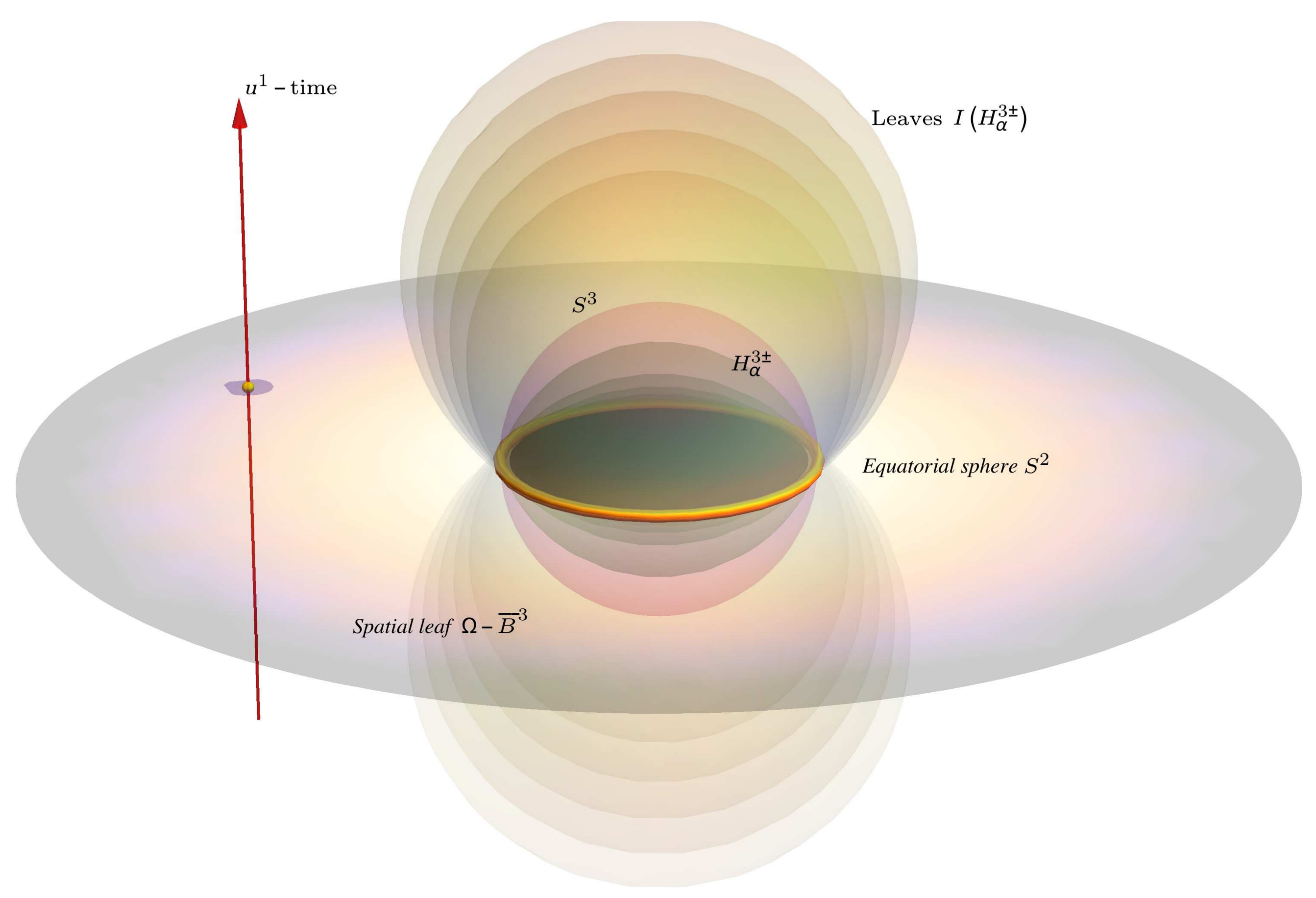
Theorem 1.

The π-orbits of $\left[{\widehat{G}}_{\tau }^{+}\right]$ in $B^4\subset \Omega$ are the three-dimensional, disjoint, simply connected and connected sets $H_{\alpha }^{3+}$, $H_{\alpha }^{3-}$ and $B^3\cap E^{0,3}$ where $H_{\alpha }^{3+}$ (resp. $H_{\alpha }^{3-}$) is the north (resp. south) hemisphere of $S_{\alpha }^3$, i.e., the set of points $u\in S_{\alpha }^3$ such that $u^{1}0$ (resp. $u^{1}0$). Note that $B^3\cap E^{0,3}$ is the limit case in $B^4$ of $H_{\alpha }^{3\pm }$ whenever α tends to infinity. Then, we denote by $H_{\infty }^3$ the leaf such that $H_{\infty }^3\equiv B^3\cap E^{0,3}$.

Proof. 

Let u be a point in $H_{\alpha }^{3\pm }$. Then, because ${\pi }_{/\mathfrak{Z}}$ is a diffeomorphism between $B^4$ and $\mathfrak{Z}$ there exists a unique point $U\in \mathfrak{Z}$ such that $\pi \left(U\right)=u$. From the algebraic definition of $S_{\alpha }^3$ and the quadratic form Q we find that U is necessarily such that ${\left(U^1\right)}^2=1/({\alpha }^2-1)$. Hence, the set of points $U={\pi }_{/\mathfrak{Z}}^{-1}\left(u\right)$ where $u\in H_{\alpha }^{3\pm }$ are elements of the hyperboloid defined by equation ${\left(U^0\right)}^2-{\sum }_{i=2}^4{\left(U^i\right)}^2={\alpha }^2/({\alpha }^2-1)$. However, ${\widehat{G}}_{\tau }^{+}\cap SL(5,\mathbb{R})$ acts transitively on this hyperboloid. Thus, $\left[{\widehat{G}}_{\tau }^{+}\right]$ acts transitively on any $H_{\alpha }^{3\pm }$. It is the same for $B^3\cap E^{0,3}$ since it is the limit case ${\alpha }^2/({\alpha }^2-1)\to 1$ whenever $\alpha \to \infty$. ☐

Corollary 1.

The σ-orbits of $\left[{\widehat{G}}_{\tau }^{+}\right]$ in Ω relative to the representation $〚〛$ are the spacelike hyperplanes ${\mathfrak{H}}_k^{ϵ}$ such that $p\left(u\right)=k⩾1$ and $sgn\left(u^1\right)=ϵ$. Moreover, we have $〚\mathfrak{A}{〛}^{*}\left(d{\tau }^2\right)=d{\tau }^2$ on Ω for any $\mathfrak{A}\in {\widehat{G}}_{\tau }^{+}$ and each ${\mathfrak{H}}_k^{\pm }$ is diffeomorphic to the leaf $H_{\alpha }^{3\pm }$ such that $k=({\alpha }^2+1)/({\alpha }^2-1)$.

Proof. 

These assertions come simply from the fact that map $\mathfrak{a}\equiv \pi \circ \sigma$ is a diffeomorphism and from Theorem 1. ☐

Corollary 2.

Let $\widehat{\mathcal{O}}\equiv \{H_{\alpha }^{3\pm },1\left|\alpha \right|⩽+\infty \}$ be the topological leaf space of π-orbits (leaves) $H_{\alpha }^{3\pm }$ in $B^4$. Then, the leaf space $\widehat{\mathcal{O}}$ is a Hausdorff space of which the leaves are not separated by closed neighborhoods on ${\overline{B}}^4$. Moreover, the π-foliation on $B^4$ is open, connected, transversally oriented (by $\left|\alpha \right|-1\in {\mathbb{R}}^{+*}$) and saturated in $B^4$.

Proof. 

Indeed, we have $B^4={\bigcup }_{\left|\alpha \right|=1}^{+\infty }{H}_{\alpha }^{3\pm }$ and $\left[{\widehat{G}}_{\tau }^{+}\right]$ operates continuously on $B^4$ via the representation $\left[\right]$. Then, for the leaf space $\widehat{\mathcal{O}}\equiv B^4\setminus \left[{\widehat{G}}_{\tau }^{+}\right]$ to be Hausdorff, it is necessary and sufficient (8, I.52 Prop. 1, I.55 Prop. 8 [16]) that the graph set $\left\{(u,u^{\prime })\in B^4\times B^4/u^{\prime }=\left[g\right].u,\left[g\right]\in \left[{\widehat{G}}_{\tau }^{+}\right]\right\}$ of the continuous action of $\left[{\widehat{G}}_{\tau }^{+}\right]$ is closed in $B^4\times B^4$, i.e., that each orbit $H_{\alpha }^{3\pm }$ is closed; what they are on $B^4$. Now, these leaves $H_{\alpha }^{3\pm }$ are neither open nor closed in ${\overline{B}}^4$ since any neighborhood (in the topology on ${\overline{B}}^4$ induced by that of $\Omega$) in ${\overline{B}}^4$ of point $u_0$ in the equatorial 2-sphere $S^2\subset S^3=\partial {\overline{B}}^4$ intersects all the leaves $H_{\alpha }^{3\pm }$. Then the latter are not separated by closed neighborhoods in ${\overline{B}}^4$. On the contrary, there would exist two closed neighborhoods $U_{\alpha }^{3\pm }$ of $H_{\alpha }^{3\pm }$ and $U_{{\alpha }^{\prime }}^{3\pm }$ of $H_{{\alpha }^{\prime }}^{3\pm }$ such that $U_{\alpha }^{3\pm }$ and $U_{{\alpha }^{\prime }}^{3\pm }$ are disjoint. However, all such closed neighborhoods contain the adherences ${\overline{H}}_{\alpha }^{3\pm }$ that intersect in $S^2$. ☐

Moreover, we have the following inversions:

• the inversion between $H_{\alpha }^{3+}$ and $H_{\alpha }^{3-}$ is obtained by the $u^1$-time inversion $T:(u^1,u^i)⟶(-u^1,u^i)$ (where $i=2,3,4$),
• the space inversion $P:u\equiv (u^1,u^i)⟶(u^1,-u^i)$ (where $i=2,3,4$) on each leaf $H_{\alpha }^{3\pm }$, and
• the inversion I in the 3-sphere $S^3$ that is the map $I:\left(u^i\right)\in {\overline{B}}^{4*}⟶(u^i/R^2)\in \Omega -B^4$ where $R^2\equiv {\sum }_{j=1}^4{\left(u^j\right)}^2$.

We can characterize more the matrices $\mathfrak{A}$ of the group ${\widehat{G}}_{\tau }^{+}$. They must preserve the two quadratic forms Q and $\tilde{Q}$ up to a same conformal factor. For this last reason, this implies that $\tilde{Q}-Q$ and $\tilde{Q}+Q$ are also preserved up to same conformal factors. Consequently, the spaces $U^1=0$ and $U^0=U^2=U^3=U^4=0$ are proper spaces and the matrices $\mathfrak{A}$ are then completely reducible. They are matrices such that ${\mathfrak{A}}_{\alpha }^1={\mathfrak{A}}_1^{\alpha }=0$ whenever $\alpha \ne 1$ and ${\mathfrak{A}}_1^1\ne 0$. In addition, their first minors, obtained by deleting the second raws and second columns associated with the coordinate $U^1$ are elements of ${\mathbb{R}}^{*}\times O(1,3)$. Note that the group $O(1,3)$ acts in two distinct ways on inhomogeneous coordinates: by homographies and as invariance subgroup of the quadratic forms Q and $\tilde{Q}$, and linearly as invariance group of the Lorentzian metric $d{\tau }^2$.

Furthermore, we restrict the group G to the subgroup $G_{\tau }^{+}\equiv {\widehat{G}}_{\tau }^{+}\cap G$ of which the matrices $\mathfrak{A}\in {\widehat{G}}_{\tau }^{+}$ have their coefficients ${\mathfrak{A}}_i^0$ and ${\mathfrak{A}}_0^i$ for $i=2,3,4$ vanishing. Hence, considering the restriction to $\left\{(0,0)\right\}\times {\mathbb{R}}^3$ of the action of $G_{\tau }^{+}$, then $G_{\tau }^{+}$ restricts to the group ${\mathbb{R}}^{*}\times O\left(3\right)$. Moreover, $\left[G_{\tau }^{+}\right]$ is the group of (general) homologies preserving the origin e of the system of Riemann normal coordinates (note that all homologies leaving variable fixed points do not form a group). Then, the coset space $[{\widehat{G}}_{\tau }^{+}/G_{\tau }^{+}]$ is the sub-group of elations (special homologies) preserving the origin e to which corresponds the group ${\widehat{G}}_{\tau }^{+}/G_{\tau }^{+}$ of boosts analogous only to those in relativity.

Definition 5.

We call “pseudo-hyperbolic space” $H^{1,3}$ the pseudo-Riemannian manifold Ω equipped with the Lorentzian metric $d{\tau }^2$.

We can note that this pseudo-Riemannian space $H^{1,3}$ is neither a anti-de Sitter space nor any of its projections on a particular projective space. In fact, we are in an unusual situation in which we have the Euclidean space ${\mathbb{R}}^5$ on which is defined the metric $d{\tilde{s}}^2$ which is the one used to define the non-simply connected anti-de Sitter space $Ad{S}_4$, but we are not using the pull-back which defines this space as a variety of dimension 4; namely the pull-back by a section like the section $\left(u^i\right)\in {\mathbb{R}}^4⟶(U^0=\sqrt{1+{\sum }_2^4{\left(u^i\right)}^2-{\left(u^1\right)}^2},U^i=u^i)\in {\mathbb{R}}^5$. In fact, we use the section $\sigma$ resulting from the definition of hyperbolic space $H^4$ which is simply connected and advantageous from the topological point of view to return to the entire simply connected space ${\mathbb{R}}^4$ specific to Riemann normal coordinates. The price to pay is a non-transitive action of invariance groups and the existence of a foliation on ${\mathbb{R}}^4$. This is a disadvantage from the point of view of group actions but this disadvantage could turn into an advantage in physics as we will see later.

In other words, there is a kind of competition between the pseudo-Riemannian structure on one side and the projective structure on the other and, metaphorically, there is a kind of “peace agreement” along the leaves only.

In addition, we define the coefficients $g_{ij}\left(u\right)$ such that

$$d{\tau }^2\equiv \sum _{i,j=1}^4{g}_{ij}\left(u\right)d{u}^{i}d{u}^j.$$

(9)

Thus, we obtain

$$\left\{\begin{array}{ccc}\hfill g_{11}& =1+\frac{{\left(u^1\right)}^2}{\chi {\left(u\right)}^2},\hfill & \\ \hfill g_{ii}& =\frac{{\left(u^i\right)}^2}{\chi {\left(u\right)}^2}-1,\hfill & \hfill (i\ne 1)\\ \hfill g_{ij}& =\frac{u^i{u}^j}{\chi {\left(u\right)}^2},\hfill & \hfill (i\ne j)\end{array}\right.$$

(10)

where $\chi {\left(u\right)}^2\equiv 1+{\sum }_{i=1}^4{\left(u^i\right)}^2$. Then, in particular, we obtain from $d{\tau }^2$ its determinant and the non-negative scalar curvature $S_c$ such that

$$det\left(d{\tau }^2\right)=-\frac{(1+2{\left(u^1\right)}^2)}{\chi {\left(u\right)}^2},S_c=\frac{12{\left(u^1\right)}^2}{{\left(2{\left(u^1\right)}^2+1\right)}^2}.$$

(11)

Hence, our approach differs from those usually considered in general relativity with anti-de Sitter spaces. Then, it suffices to restrict the group of homographies to the group $\left[{\widehat{G}}_{\tau }^{+}\right]\subset SL(5,\mathbb{R})=PGL(5,\mathbb{R})$ compatible with the invariance of the Lorentzian metric $d{\tau }^2$ on the $\sigma$-orbits of $\left[{\widehat{G}}_{\tau }^{+}\right]$.

Finally, we give the following definition of a projective geometric object.

Definition 6.

A geometric object, e.g., a tensor, is said projectively invariant if it is invariant with respect to $\left[{\widehat{G}}_{\tau }^{+}\right]$ on all σ-orbits of $\left[{\widehat{G}}_{\tau }^{+}\right]$ in $H^{1,3}$. It is said to be partially projectively invariant if it is invariant with respect to a proper subgroup of $\left[{\widehat{G}}_{\tau }^{+}\right]$.

In particular, a geometric object on the union $\Omega$ of $\sigma$-orbits, can be non-continuous on $\Omega$ but continuous only when restricted to any spacelike leaf ${\mathfrak{H}}_k^{\pm }$, i.e., we consider the case where only the discrete topology on $\Omega$ with respect to the $\sigma$-foliation remains.

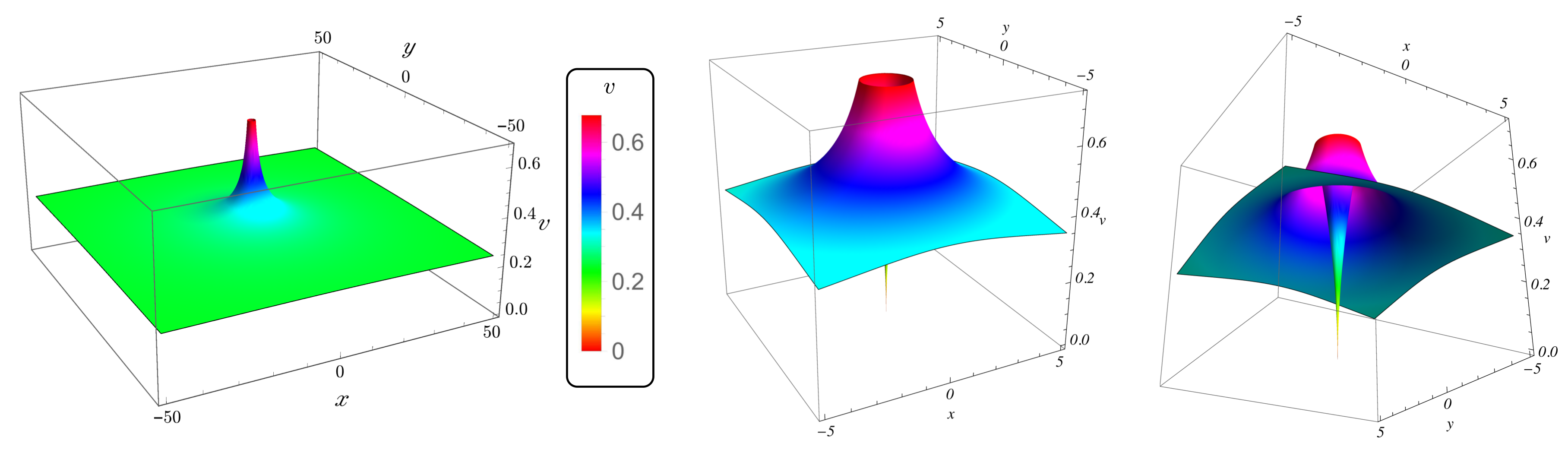
2.5. A Particular Discontinuous Projectively Invariant Lorentzian Metric

We have shown the map $\mathfrak{a}:\Omega ⟶B^4$ is a diffeomorphism and its inverse ${\mathfrak{a}}^{-1}:\left(u^i\right)\in B^4⟶\left(u^{\prime i}\right)\in \Omega$ is defined by the relations $u^{\prime i}\equiv {\mathfrak{a}}^{-1}{\left(u\right)}^i=u^i/\sqrt{1-{\sum }_{k=1}^4{\left(u^k\right)}^2}$. Then, the metric $d{\widehat{h}}^2\equiv {\mathfrak{a}}^{-1*}\left(d{\tau }^2\right)$ defined on $B^4$ is continuous and projectively invariant along each leaf $H_{\alpha }^{3\pm }$ with respect to the group $\left[{\widehat{G}}_{\tau }^{+}\right]$ with the representation $\left[\right]$. Indeed, from relation $\mathfrak{a}\circ 〚\mathfrak{A}〛=\left[\mathfrak{A}\right]\circ \mathfrak{a}$, we deduce that ${\left[\mathfrak{A}\right]}^{*}\left(d{\widehat{h}}^2\right)={\left[\mathfrak{A}\right]}^{*}\circ {\mathfrak{a}}^{-1*}\left(d{\tau }^2\right)={\mathfrak{a}}^{-1*}\circ 〚\mathfrak{A}{〛}^{*}\left(d{\tau }^2\right)={\mathfrak{a}}^{-1*}\left(d{\tau }^2\right)=d{\widehat{h}}^2$. However, $d{\widehat{h}}^2$ is necessarily not continuous on the equatorial sphere $S^2\subset S^3=\partial {\overline{B}}^4$ because the leaves $H_{\alpha }^{3\pm }$ cannot be separated by closed neighborhoods on ${\overline{B}}^4$ and, more specifically, on any neigbhourhood of the spacelike equatorial sphere $S^2\subset E^{0,3}$. Then, considering the inversion I in the 3-sphere $S^3$, we define $d{\check{h}}^2\equiv I^{-1*}\left(d{\widehat{h}}^2\right)$ on $\Omega -{\overline{B}}^4$ which is therefore no more continuous on $S^2$ but also projectively invariant along each leaf $I\left(H_{\alpha }^{3\pm }\right)\subset \Omega -{\overline{B}}^4$ with respect to the group $\left[{\widehat{G}}_{\tau }^{+}\right]$ with again the representation $\left[\right]$. Besides, we can note that $I\left(H_{\infty }^3\right)=E^{0,3}-{\overline{H}}_{\infty }^3$. Indeed, I commutes with $\left[\right]$, i.e., for all $\mathfrak{A}$ we have $\left[\mathfrak{A}\right]\circ I=I\circ \left[\mathfrak{A}\right]$. Then, $\Omega -S^3$ equipped with the metric $d{h}^2\equiv (d{\check{h}}^2,d{\widehat{h}}^2)$ on $(\Omega -{\overline{B}}^4)\times B^4$ is a Lorentzian metric that diverges to infinity on $S^3$; which can be shown by a direct calculation using a symbolic calculation software (SCS). In addition, we find that $d{\widehat{h}}^2$ is the Minkowski metric at $u=0$, i.e., at the event e origin of the Riemann normal coordinates. We can say that $d{h}^2$ is topologically singular on $S^3$. Furthermore, we obtain a $\pi$-foliation and a representation $\left[\right]$ of $\left[{\widehat{G}}_{\tau }^{+}\right]$ which extend from $B^4$ to $\Omega -{\overline{B}}^4$ via inversion I.

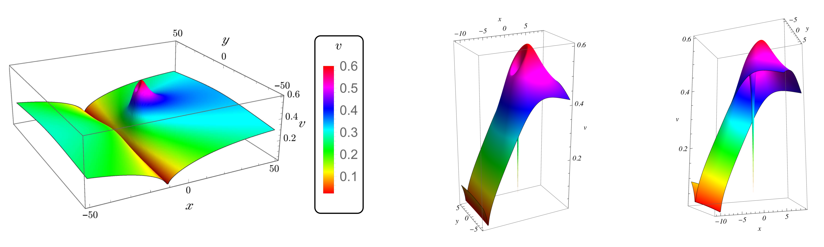
A natural way to get around this singularity problem on $S^3$ is to consider a class of conformal metrics $d{\widehat{\nu }}^2\equiv {\Psi }^2\left(u\right)d{\widehat{h}}^2$ defined from $d{\widehat{h}}^2$ and suitable functions $\Psi$. The latter must be invariant with respect to $\left[{\widehat{G}}_{\tau }^{+}\right]$ with representation $\left[\right]$ to preserve the $\pi$-foliation. Hence, $\Psi$ must be a function $\Xi \left(q\right)$ of the fraction $q\left(u\right)$ from which the leaves were deduced. Besides, a direct computations using a SCS shows that the determinant of $d{\widehat{h}}^2$ and its scalar curvature ${\widehat{S}}_c$ are such that

$$\begin{array}{cc}\hfill det\left(d{\widehat{h}}^2\right)& =-\frac{{\left(R^2+1\right)}^2\left({(R^2-1)}^2+2{\left(u^1\right)}^2\right)}{\left({(R^2-1)}^2+R^2\right){\left(R^2-1\right)}^{10}}\equiv \frac{K\left(u\right)}{{(R-1)}^{10}},\hfill \\ \hfill {\widehat{S}}_c& =\frac{12{\left(u^1\right)}^2{(R^2-1)}^2}{\left({(R^2-1)}^2+2{\left(u^1\right)}^2\right)},\hfill \end{array}$$

(12)

where $R^2={\sum }_{k=1}^4{\left(u^k\right)}^2$ and K is then such that $\left|K\right(u\left)\right|+\infty$ on ${\overline{B}}^4$. In addition, the metric $d{\widehat{h}}^2$ is the Minkowski metric at $u\equiv 0$. 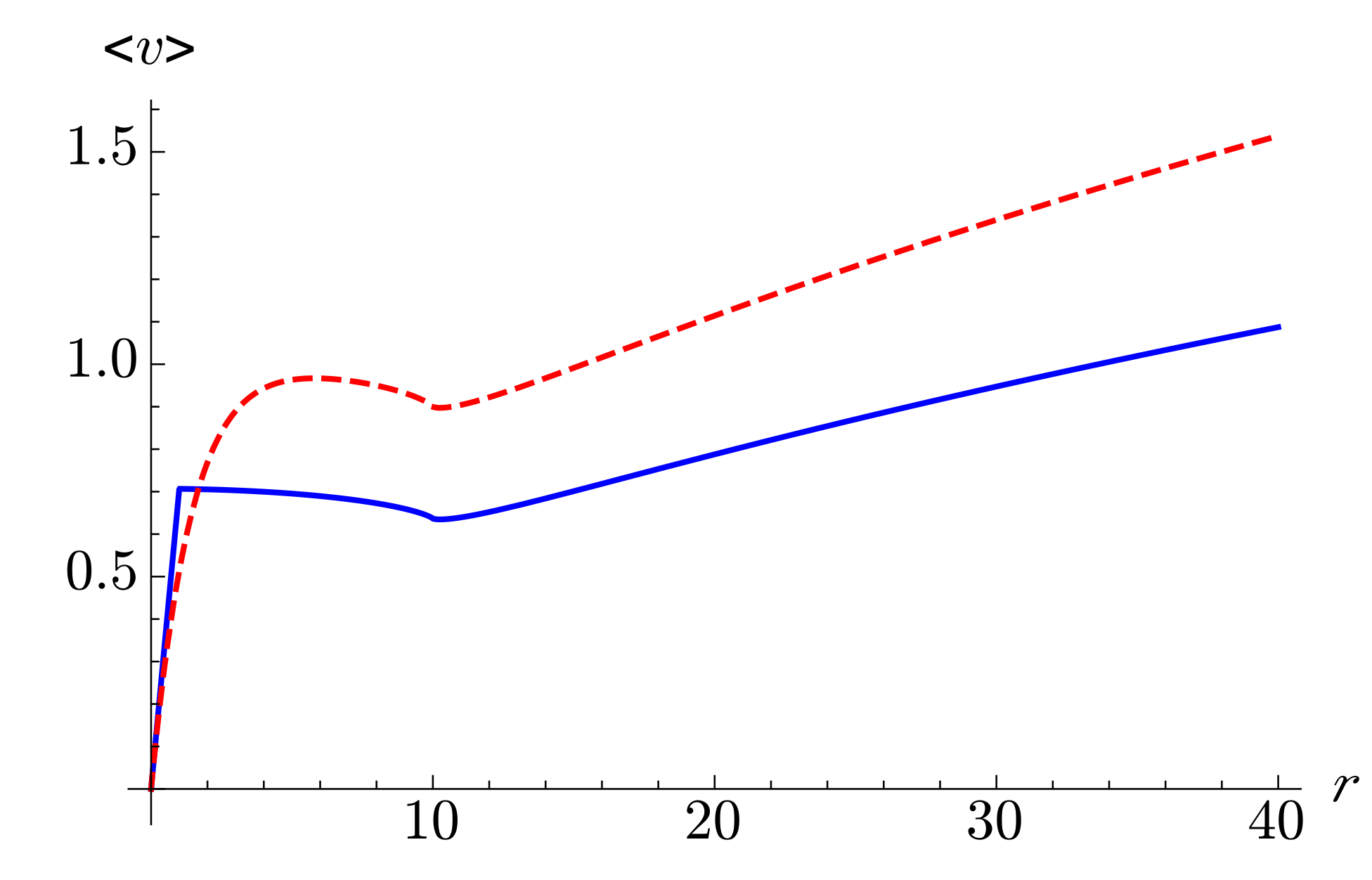Therefore, from the algebraic expression for $q\left(u\right)$ which is of the form ${\left(u^1\right)}^2/(1-R)$ in the vicinity of $R=1$, to obtain a metric $d{\widehat{\nu }}^2$ with a finite determinant on ${\overline{B}}^4$, then the function $\Xi$ must be such that

$$\Xi \left(q\right)\equiv \frac{C\left(q\right)}{q^{5/4}},$$

(13)

where $C\left(q\right)$ is a continuous function, bounded on $[1,+\infty ]$ and such that $C(+\infty )=c_{\infty }\ne 0$ whenever $u^1\ne 0$. Moreover, if $\left|C\right(1\left)\right|=1$ then $d{\widehat{\nu }}^2$ is the Minkowski metric at $u=0$. Unfortunately, the finiteness of $det\left(d{\widehat{\nu }}^2\right)$ cannot be maintained if $u^1=0$ and $R\ne 0$, i.e., on the equatorial sphere $S^2\subset E^{0,3}$. Hence, the metric $d{\widehat{\nu }}^2$ is defined on ${\overline{B}}^4-S^2$ and we define $d{\check{\nu }}^2\equiv I^{-1*}\left(d{\widehat{\nu }}^2\right)$ on $\Omega -(B^4\cup S^2)$. Then, we define the following particular pseudo-Riemanniann manifold.

Definition 7.

We call “singular pseudo-hyperbolic space” $H_s^{1,3}$ the pseudo-Riemannian manifold Ω equipped with the Lorentzian metric $d{\nu }^2\equiv (d{\check{\nu }}^2,d{\widehat{\nu }}^2)$ topologically singular on $S^2$.

We then discuss in Section 5 a possible relationship between this singular pseudo-hyperbolic space $H_s^{1,3}$ and the admissible metrics in black hole theory.

In addition, we can say that the open ball $B^4$ is equipped with an orbifold structure by considering the finite group $\Gamma$ having inversion I as generator. Then, we have $B^4\equiv H_s^{1,3}/\Gamma$.

3. The Invariant Tensors with Respect to Homographies

3.1. Introduction—Invariance of Families of Tensors or Tensors Fields

So far only one system of Riemann normal coordinates explicitly attached to point e has been considered. The singular metrics $d{h}^2$ or $d{\nu }^2$ (resp. $d{\tau }^2$) are metric fields defined on the space $\Omega$ also attached to this point. We have shown that these fields of metrics are invariant with respect to the group $\left[{\widehat{G}}_{\tau }^{+}\right]$ of homographies with representation $\left[\right]$ (resp. $〚〛$). These fields therefore have components that are equivariant with respect to this same group, i.e., we typically have relations such as ${\omega }_{ij}(\left[\mathfrak{A}\right].u)\equiv {\mathfrak{M}}_i^k\left(u\right){\mathfrak{M}}_j^h\left(u\right){\omega }_{kh}\left(u\right)$ for their components $\omega$ and for any element $\mathfrak{A}\in {\widehat{G}}_{\tau }^{+}$ where the matrices $\mathfrak{M}$ such that $det\mathfrak{M}\ne 0$ are the Jacobian matrices univocally defined from the homographies $\left[\mathfrak{A}\right]$ (resp. $〚\mathfrak{A}〛$).

Now, if we consider the particular case of a force as the gravitational force, the latter is attached to a point, the “source” point e in this case, and it applies to another mass at a “target” point $p\in \Omega$. Of course, this is not a force field on $\Omega$. Indeed, we can perfectly have a second mass at another target point $p^{\prime }$ and therefore we have a second gravitational force always attached to the single source point e. So we have a family of gravitational forces all attached to the same source point e. The fact that the general mathematical expression of gravitational forces does not change according to the selected variable target point p means that we have a particular invariance of this family. It is therefore somehow a gravitational force attached to the single source point e that is a field because parameterized by the selected target point $p\in \Omega$ but not a force field on $\Omega$ giving in that case only, a force vector attached to each source point in $\Omega$. This may seem unusual, but it is clear experimentally that several different forces can be applied to a mass. That only the single total applied force is considered does not change the fact that originally several distinct forces apply, each associated with different target points p. This is especially true since the general formula for this single total force will not take the general mathematical form of the different forces of which it is made up.

Naturally, the group of invariance that must be considered is the group $\left[{\widehat{G}}_{\tau }^{+}\right]$ in order to define this family of forces at e as a projective geometric object. In addition, this family will be associated with a family of equivariant components with respect to this same group applied on the set of target points $p\in \Omega$. Thereafter, choosing a particular force in this family, this force vector will be used in some way as a germ at the source point e to infer a particular force fields class defined on the spacetime manifold $\mathcal{M}$. In what follows, we will focus only on the invariance of these force families with respect to group $\left[{\widehat{G}}_{\tau }^{+}\right]$ with representation $\left[\right]$ attached to the single origin source point $e\in \mathcal{M}$.

3.2. Invariant Families of Tensors Attached to a Single, Given Point

Now, the objective is to determine invariant vectors with respect to $\left[{\widehat{G}}_{\tau }^{+}\right]$ and representation $\left[\right]$ (from which invariance relative to representation $〚〛$ is deduced with the map $\mathfrak{a}$) in order to determine a modification of Newton’s law compatible with the projective structure. However, the Newtonian force being a 3-vector, only a group isomorphic to the group of rotations $SO(3,\mathbb{R})$ will be considered. Hence, only the stronger invariance with respect to the group $\left[G_{\tau }^{+}\right]$ of homologies must be considered. In particular, the latter keeps conformally invariant the time dependent Euclidean spatial metric

$$d{\widehat{\ell }}^2=\sum _{i,j=2}^4{\widehat{\gamma }}_{ij}\left(u\right)d{u}^{i}d{u}^j,$$

(14)

where ${\widehat{\gamma }}_{ij}\equiv {\widehat{\omega }}_{1j}{\widehat{\omega }}_{1i}/{\widehat{\omega }}_{11}-{\widehat{\omega }}_{ij}$ ($i,j=2,3,4$) and ${\widehat{\omega }}_{\alpha \beta }$ are the components of the metric $d{\widehat{h}}^2$ defined in $B^4$. Using a SCS, we find that

$$det\left(d{\widehat{\ell }}^2\right)=\frac{{(R^2+1)}^2\left({(R^2-1)}^2+2{\left(u^1\right)}^2\right)}{{\left(R^2-1\right)}^{6}D(R,u^1)},$$

(15)

where

$$\begin{array}{c}D(R,u^1)=R^8-(8{\left(u^1\right)}^2+3)R^6+(8{\left(u^1\right)}^4+13{\left(u^1\right)}^2+4)R^4\hfill \\ -(8{\left(u^1\right)}^4+10{\left(u^1\right)}^2+3)R^2+8{\left(u^1\right)}^4+5{\left(u^1\right)}^2+1,\hfill \end{array}$$

(16)

where $R^2\equiv {\sum }_{j=1}^4{\left(u^j\right)}^2$. Moreover, if $u^2=u^3=u^4=0$ and ${\left(u^1\right)}^{2}1$ then we obtain in particular:

$$d{\widehat{\ell }}^2\equiv \frac{1}{{\left({\left(u^1\right)}^2-1\right)}^2}\sum _{k=2}^{4}d{\left(u^k\right)}^2.$$

(17)

It can be shown by direct numerical computations that $D(R,u^1)0$ whenever $R^{2}1$ and ${\left(u^1\right)}^{2}1$. Hence, $det\left(d{\widehat{\ell }}^2\right)$ is positive in $B^4$. In addition, its scalar curvature ${\widehat{S}}_{\ell }$ is of the form:

$${\widehat{S}}_{\ell }(R,u^1)\equiv \frac{N(R,u^1)}{{(R^2+1)}^3\left({(R^2-1)}^2+2{\left(u^1\right)}^2\right)},$$

(18)

where $N(R,u^1)$ is a polynomial with relative integer coefficients and of degree 14 with respect to R and of degree 8 with respect to $u^1$. Numerical computations again show that $N(R,u^1)$ is negative whenever $R1$ and ${\left(u^1\right)}^{2}1$ and vanishes for $R=1$ and $u^1=0$. In addition, we obtain $N(R=1,u^1)=768{\left(u^1\right)}^6({\left(u^1\right)}^2-1)$ and thus ${\widehat{S}}_{\ell }(R=1,u^1)\equiv 48{\left(u^1\right)}^4({\left(u^1\right)}^2-1)$ meaning, in particular, that ${\widehat{S}}_{\ell }$ vanishes on the spacelike equatorial sphere $S^2$. Using inversion I, we deduce its counterpart $d{\check{\ell }}^2$ on $\Omega -{\overline{B}}^4$ from $d{\check{h}}^2$ with also a negative scalar curvature since the inversion I is a conformal map. Hence, ${\widehat{S}}_{\ell }$ is negative or null and bounded on ${\overline{B}}^4$. In addition, that the metric $d{\widehat{\ell }}^2$ is invariant with respect to $O\left(3\right)$ is well known. Its conformal invariance with respect to $\left[G_{\tau }^{+}\right]$ comes simply from the fact that $G_{\tau }^{+}$ is isomorphic to ${\left({\mathbb{R}}^{*}\right)}^3\times O\left(3\right)$ and that the three scale factors belonging to ${\left({\mathbb{R}}^{*}\right)}^3$ are distinct in full generality.

Now, we can define projective families of vectors attached to source origin point e as $\left[G_{\tau }^{+}\right]$-invariant vector fields with respect to target points p starting from the following general framework.

3.2.1. General Framework for Invariant Projective Vector Fields

The general results presented in this paragraph are well known and are standard constructions. We present them briefly nevertheless to fix the ideas and the notations, and to indicate very elementary but essential properties which will be used in part in the continuation. The fundamental and technical aspects are related to the theory of moduli spaces of projective invariants [17,18] and projective schemes [19].

Let $\widehat{V}$ be a vector field on ${\mathbb{R}}^5$ such as $\widehat{V}\left(U\right)\in {\mathbb{R}}^5$ for $U\equiv \left(U^{\alpha }\right)\in {\mathbb{R}}^5$ given. Then, if we consider formulas (2) and setting $\widehat{V}{\left(U\right)}^{\alpha }\equiv U^{\alpha }$, then $\widehat{V}$ is naturally invariant with respect to $GL(5,\mathbb{R})$ since we have $\widehat{V}\left(\mathfrak{A}U\right)\equiv \mathfrak{A}\widehat{V}\left(U\right)$ whatever is $\mathfrak{A}\in GL(5,\mathbb{R})$. Then, $\widehat{V}\left(U\right)$ is an element of the fiber over U in the so-called tautological bundle over the base space ${\mathbb{R}}^5$. Thus, any vector field ${\widehat{W}}_n$ such that ${\widehat{W}}_n\left(U\right)\equiv {\widehat{V}}_1\left(U\right)\otimes \cdots \otimes {\widehat{V}}_n\left(U\right)$ where each ${\widehat{V}}_i$ is a copy of $\widehat{V}$, i.e., ${\widehat{V}}_i\equiv \widehat{V}$, is also invariant with respect to $GL(5,\mathbb{R})$. As a result, for some indices $n\in I\subset {\mathbb{N}}^{*}$, any analytical vector field ${\widehat{IW}}_n$ which is an irreducible part of ${\widehat{W}}_n$ in ${\mathbb{R}}^5$ with respect to $GL(5,\mathbb{R})$ is also invariant with respect to $GL(5,\mathbb{R})$ and, moreover, its components are homogeneous polynomials of degree n in the variables $U^{\alpha }$.

We can generate an other class of invariant vector fields given any fixed element ${\mathfrak{A}}_0\in GL(5,\mathbb{R})$ in full generality. The matrix ${\mathfrak{A}}_0$ can depend in its definition on a set $\mathbf{k}$ of N arbitrary parameters $k^1$, $k^2$, …, $k^N$ independent of the points U unlike the most general matrices $\mathfrak{A}$ which have only numerical fixed coefficients. Or, if nevertheless ${\mathfrak{A}}_0$ depends on the points U , we consider its coefficients as homogeneous functions of degree 0 to keep the homogeneity degrees of the components of the vectors involved in the various relations of equivariance. That also means that they can depend only on the inhomogeneous coordinates $u^i$.

In other words, we consider that the whole set of $GL(5,\mathbb{R})$-invariant vector fields is a finite ${\mathcal{K}}_0$-module where ${\mathcal{K}}_0$ is the function field of homogeneous functions of degree zero with respect to variables $U^{\alpha }$.

Then, defining $\widehat{Z}$ such that $\widehat{Z}\left(U\right)\equiv {\mathfrak{A}}_0\widehat{V}\left(U\right)$ with ${\mathfrak{A}}_0$ independent of U , we obtain for any $\mathfrak{A}\in GL(5,\mathbb{R})$ the relation of equivariance $\widehat{Z}\left(\mathfrak{A}U\right)={\iota }_{{\mathfrak{A}}_0}\left(\mathfrak{A}\right)\widehat{Z}\left(U\right)$ where ${\iota }_{{\mathfrak{A}}_0}$ is the inner automorphism associated with ${\mathfrak{A}}_0$, i.e., ${\iota }_{{\mathfrak{A}}_0}\left(\mathfrak{A}\right)\equiv {\mathfrak{A}}_0\mathfrak{A}{\mathfrak{A}}_0^{-1}$. In addition, if ${\mathfrak{A}}_0\left(U\right)$ has coefficients that are homogeneous functions of degree 0 with respect to the variables $U^{\alpha }$, then we obtain also a relation of equivariance $\widehat{Z}\left(\mathfrak{A}U\right)={\iota }_{{\mathfrak{A}}_0}^{*}\left(\mathfrak{A}\right)\widehat{Z}\left(U\right)$ where ${\iota }_{{\mathfrak{A}}_0}^{*}\left(\mathfrak{A}\right)\equiv {\mathfrak{A}}_0\left(\mathfrak{A}U\right)\mathfrak{A}{\mathfrak{A}}_0^{-1}\left(U\right)$ is homogeneous of degree 0. We refer to these two cases denoting ${\iota }^{(*)}$.

Then, in the same way as for vectors ${\widehat{IW}}_n$, for some $q\in I\subset {\mathbb{N}}^{*}$, we can obtain $GL(5,\mathbb{R})$-invariant, analytical vector fields ${\widehat{IZ}}_q$ on ${\mathbb{R}}^5$.

In addition, we can obtain from $\widehat{W}$ and $\widehat{Z}$ analytical vector fields ${IW}_r^{•}\left(U\right)$ and ${IZ}_s^{•}\left(U\right)$ on ${\mathbb{R}}^5$, with values in ${\mathbb{R}}^4$, irreducible with respect to the group $GL(4,\mathbb{R})$. Their equivariance relations are then ${IW}_r^{•}\left(\mathfrak{A}U\right)=A_{\mathfrak{A}}{IW}_r^{•}\left(U\right)$ and ${IZ}_s^{•}\left(\mathfrak{A}U\right)={\iota }_{A_{{\mathfrak{A}}_0}}^{(*)}\left(A_{\mathfrak{A}}\right){IZ}_s^{•}\left(U\right)$ for some indices $r,s\in K\subset {\mathbb{N}}^{*}$ and where $\mathfrak{A}\in {\mathbb{R}}^{*}\times GL(4,\mathbb{R})$.

Besides, if we project $\widehat{V}$ onto $V\equiv \left(V^i\right)$, we deduce also for $p,m\in J\subset {\mathbb{N}}^{*}$, analytical invariant vector fields $I{W}_m\equiv \left({IW}_m^i\right)$ and ${IZ}_p\equiv \left({IZ}_p^i\right)$ on ${\mathbb{R}}^4$ with values this time in ${\mathbb{R}}^4$ and irreducible with respect to $GL(4,\mathbb{R})$ such that ${IW}_m\left(A_{\mathfrak{A}}u\right)=A_{\mathfrak{A}}{IW}_m\left(u\right)$ and ${IZ}_p\left(A_{\mathfrak{A}}u\right)={\iota }_{A_{{\mathfrak{A}}_0}}^{(*)}\left(A_{\mathfrak{A}}\right){IZ}_p\left(u\right)$ where $u\equiv \left(u^i\right)\in {\mathbb{R}}^4$.

To summarize, we have the following list of analytical $GL(5,\mathbb{R})$-invariant and $GL(4,\mathbb{R})$-invariant vector fields:

$$\begin{array}{cc}\hfill {\widehat{IW}}_n(n\in I):& {\widehat{IW}}_n\left(\mathfrak{A}U\right)=\mathfrak{A}{\widehat{IW}}_n\left(U\right),\hfill \\ \hfill {\widehat{IZ}}_q(q\in I):& {\widehat{IZ}}_q\left(\mathfrak{A}U\right)={\iota }_{{\mathfrak{A}}_0}^{(*)}\left(\mathfrak{A}\right){\widehat{IZ}}_q\left(U\right),\hfill \\ \hfill {IW}_r^{•}(r\in K):& {IW}_r^{•}\left(\mathfrak{A}U\right)=A_{\mathfrak{A}}{IW}_r^{•}\left(U\right),\hfill \\ \hfill {IZ}_s^{•}(s\in K):& {IZ}_s^{•}\left(\mathfrak{A}U\right)={\iota }_{A_{{\mathfrak{A}}_0}}^{(*)}\left(A_{\mathfrak{A}}\right){IZ}_s^{•}\left(U\right),\hfill \\ \hfill {IW}_m(m\in J):& {IW}_m\left(A_{\mathfrak{A}}u\right)=A_{\mathfrak{A}}{IW}_m\left(u\right),\hfill \\ \hfill {IZ}_p(p\in J):& {IZ}_p\left(A_{\mathfrak{A}}u\right)={\iota }_{A_{{\mathfrak{A}}_0}}^{(*)}\left(A_{\mathfrak{A}}\right){IZ}_p\left(u\right).\hfill \end{array}$$

(19)

3.2.2. Invariant Projective Vector Fields on $\Omega$

Previous vector fields are not vector fields on $\Omega$ except for vector fields ${IW}_m$ and ${IZ}_p$ but they can be nevertheless projectable on this space. For, we can consider the push-forward ${\widehat{K}}_n=\left({\widehat{K}}_n^i\right)$ of the projectable, non-analytical vector field ${({\widehat{IW}}_n^i/{\widehat{IW}}_n^0)}_{i=1,\dots ,4}$, of which the components are homogeneous fractions of degree 0 with respect to the variables $U^{\alpha }$, by the projecting map $\pi$, i.e., $K_n\left(u\right)\equiv {\pi }_{*}\left({\widehat{IW}}_n^i/{\widehat{IW}}_n^0\right)\left(u\right)$. Then, the vector field $K_n$ on $H_s^{1,3}$ is invariant with respect to homographies $\left[\mathfrak{A}\right]\in \left[G_{\tau }^{+}\right]$ only, i.e., we have

$$K_n\left(\left[\mathfrak{A}\right]\left(u\right)\right)={\tilde{A}}_{\mathfrak{A}}\left(u\right)K_n\left(u\right)$$

(20)

where ${\tilde{A}}_{\mathfrak{A}}\equiv {\lambda }_{\mathfrak{A}}{A}_{\mathfrak{A}}$ with ${\lambda }_{\mathfrak{A}}$ a real scaling function is a frame field on $H_s^{1,3}$ defined from $\mathfrak{A}$.

In the same way, we can define non-analytical, invariant vector fields $H_q\left(u\right)\equiv {\pi }_{*}\left({\widehat{IZ}}_q^i/{\widehat{IZ}}_q^0\right)\left(u\right)$ which satisfy the relations of equivariance

$$H_q\left(\left[\mathfrak{A}\right]\left(u\right)\right)={\iota }_{A_0}^{(*)}\left({\tilde{A}}_{\mathfrak{A}}\right)\left(u\right)H_q\left(u\right)$$

(21)

with respect to $\left[G_{\tau }^{+}\right]$ only.

Similarly, the following analytical vectors on $H_s^{1,3}$ are defined:

$$\begin{array}{cc}\hfill {\widehat{I}}_n\equiv {\pi }_{*}\left({\widehat{IW}}_n\right)(n\in I):& {\widehat{I}}_n\left(\left[\mathfrak{A}\right]\left(u\right)\right)=\mathfrak{A}{\widehat{I}}_n\left(u\right),\hfill \\ \hfill {\widehat{J}}_q\equiv {\pi }_{*}\left({\widehat{IZ}}_q\right)(q\in I):& {\widehat{J}}_q\left(\left[\mathfrak{A}\right]\left(u\right)\right)={\iota }_{{\mathfrak{A}}_0}^{(*)}\left(\mathfrak{A}\right){\widehat{J}}_q\left(u\right),\hfill \\ \hfill I_r^{•}\equiv {\pi }_{*}\left({IW}_r^{•}\right)(r\in K):& I_r^{•}\left(\left[\mathfrak{A}\right]\left(u\right)\right)=A_{\mathfrak{A}}{I}_r^{•}\left(u\right),\hfill \\ \hfill J_s^{•}\equiv {\pi }_{*}\left({IZ}_s^{•}\right)(s\in K):& J_s^{•}\left(\left[\mathfrak{A}\right]\left(u\right)\right)={\iota }_{A_{{\mathfrak{A}}_0}}^{(*)}\left(A_{\mathfrak{A}}\right)J_s^{•}\left(u\right).\hfill \end{array}$$

(22)

These vectors are invariant with respect to $GL(5,\mathbb{R})$. In addition, we set $I_m\equiv {IW}_m$ and $J_p\equiv {IZ}_p$ which are $GL(4,\mathbb{R})$-invariant analytical vectors.

Then, fields of conformally invariant polynomials or polynomial fractions on $H_s^{1,3}$ can be deduced associated with the groups $\left[{\widehat{G}}_{\tau }^{+}\right]$, $\left[G_{\tau }^{+}\right]$ and $G_{\tau }^{+4}\equiv GL(4,\mathbb{R})\bigcap G_{\tau }^{+}$ (notation: conf. invts = “conformally invariants”) :

$$\begin{array}{ccc}\hfill \left[{\mathfrak{G}}_{\tau }^{•}\right]& =\left\{d{\widehat{\nu }}_e^2(X,Y)/X,Y=I_r^{•}\mathrm{or}{J}_s^{•}\right\},\hfill & \left[{\widehat{G}}_{\tau }^{+}\right]-\mathit{conf}.\mathit{invts},\hfill \\ \hfill [{\mathfrak{G}}_{\tau }]& =\left\{d{\widehat{\nu }}_e(X,Y)/X,Y=K_n,H_q,I_r^{•},\mathrm{or}{J}_s^{•}\right\},\hfill & \left[G_{\tau }^{+}\right]-\mathit{conf}.\mathit{invts},\hfill \\ \hfill {\mathfrak{G}}_{\tau }& =\left\{d{\widehat{\nu }}_e(X,Y)/X,Y=I_m,J_p,K_n,H_q,I_r^{•},\mathrm{or}{J}_s^{•}\right\},\hfill & G_{\tau }^{+4}-\mathit{conf}.\mathit{invts},\hfill \\ \hfill [{\mathfrak{G}}_{\ell }]& =\left\{d{\widehat{\ell }}_{e}2(X,Y)/X,Y=K_n,H_q,I_r^{•},\mathrm{or}{J}_s^{•}\right\},\hfill & \left[G_{\tau }^{+}\right]-\mathit{conf}.\mathit{invts},\hfill \\ \hfill {\mathfrak{G}}_{\ell }& =\left\{d{\widehat{\ell }}_e(X,Y)/X,Y=I_m,J_p,K_n,H_q,I_r^{•},\mathrm{or}{J}_s^{•}\right\},\hfill & G_{\tau }^{+4}-\mathit{conf}.\mathit{invts}.\hfill \end{array}$$

(23)

Note that $d{\widehat{\nu }}_e$ and $d{\widehat{\ell }}_e$ are, respectively, the Minkowski metric and the spatial canonical Euclidean metric at $e\equiv (u^i=0)$.

These fields will be of great importance within this framework of projective geometry because it will be the fields of functions onto which modified Newton’s forces will be defined.

3.3. A Particular Modified Newton’s Law

We can present an example of fractions deduced from the vector field $H_1$ associated with the linear map ${\mathfrak{A}}_0(\mathbf{k},U)$ such that

$${\mathfrak{A}}_0\left(\mathbf{k}\right)=\left(\begin{array}{ccccc}{a}_0^0(\mathbf{k},U)& a_1^0(\mathbf{k},U)& a_2^0(\mathbf{k},U)& a_3^0(\mathbf{k},U)& a_4^0(\mathbf{k},U)\\ 0& 1& 0& 0& 0\\ 0& 0& 1& 0& 0\\ 0& 0& 0& 1& 0\\ 0& 0& 0& 0& 1\end{array}\right),$$

(24)

where $a_0^0(\mathbf{k},U)U^0\ne 0$, ${\sum }_{i=1}^4{a}_i^0(\mathbf{k},U)u^i\ne 0$, $\mathbf{k}$ is a set of parameters and the functions $a_{\alpha }^0$ are homogeneous functions of degree 0 with respect to the variables $U^{\beta }$. Then, we obtain after the push-forwards by $\pi$:

$$H_1\left(u\right)=\frac{1}{\left(c_0(\mathbf{k},u)+{\sum }_{i=1}^4{c}_i(\mathbf{k},u)u^i\right)}\left(\begin{array}{c}{u}^1\\ u^2\\ u^3\\ u^4\end{array}\right),$$

(25)

where $a_{\alpha }^0\equiv c_{\alpha }$. Therefore, from (17) at e , we deduce the the fraction in $\left[{\mathfrak{G}}_{\ell }\right]$:

$$d^2(u,\mathbf{k})=\frac{{\sum }_{i=2}^4{\left(u^i\right)}^2}{{\left(c_0(\mathbf{k},u)+{\sum }_{i=1}^4{c}_i(\mathbf{k},u)u^i\right)}^2}.$$

(26)

Then, setting $u^1\equiv t$, $u^2\equiv x$, $u^3\equiv y$, $u^4\equiv z$, $c_1\equiv c_t(\mathbf{k},u)$, $c_2\equiv c_x(\mathbf{k},u)$, $c_3\equiv c_y(\mathbf{k},u)$, $c_4\equiv c_z(\mathbf{k},u)$ and $r^2\equiv {\sum }_{i=2}^4{\left(u^i\right)}^2$ we obtain the fraction

$$d^2(t,x,y,z)=\frac{r^2}{{\left(c_0+c_{t}t+c_{x}x+c_{y}y+c_{z}z\right)}^2}.$$

(27)

Then, we deduce the modified Newton’s law ${\overrightarrow{\mathbf{F}}}_{a/b}$ invariant with respect to $\left[G_{\tau }^{+}\right]$:

$${\overrightarrow{\mathbf{F}}}_{a/b}=\mathcal{G}{m}_a{m}_b\frac{{\left(c_0+c_{t}t+c_{x}x+c_{y}y+c_{z}z\right)}^2}{r^2}\overrightarrow{\mathbf{v}},$$

(28)

where $\mathcal{G}$ is the universal gravitational constant and $\overrightarrow{\mathbf{v}}$ is the unit vector directed along the line joining the positions of the two punctual masses $m_a$ and $m_b$.

We focus mainly on two particular classes of modified Newton’s laws, the first called “isotropic” class, and the other, naturally, “anisotropic” class.

3.3.1. The Isotropic Class

In this case, we want a force invariant with respect to rotations which is the most natural way to change Newton’s law in a first approach. This also makes it possible to compare these modifications with others already proposed such as those resulting from MOND theories for example. Thus, we can set for instance $c_0(\mathbf{k},u)\equiv k_0\ne 0$, $c_t(\mathbf{k},u)\equiv k_t$, $c_x(\mathbf{k},u)\equiv -k_{x}r/x$, $c_y(\mathbf{k},u)\equiv -k_{y}r/y$ and $c_z(\mathbf{k},u)\equiv -k_{z}r/z$ where the k’s are constant or depend only on the time t and radius r. These c functions clearly originate from homogeneous functions $a_{\alpha }$ of degree 0 with respect to the variables $U^{\alpha }$. Then, we obtain

$${\overrightarrow{\mathbf{F}}}_{a/b}=\mathcal{G}{m}_a{m}_b\frac{{\left(k_0+k_{t}t-kr\right)}^2}{r^2}\overrightarrow{\mathbf{v}},$$

(29)

where $k\equiv k_x+k_y+k_z$.

3.3.2. The Anisotropic Class

Out of curiosity, we also consider this case of a modified Newton’s law not invariant with respect to rotations, but nevertheless remaining conformally invariant with respect to $\left[G_{\tau }^{+}\right]$. This case may seem irrelevant to consider given what we know about Newton’s force. However, in fact, some anisotropy of the modified Newton’s force could perhaps provide one of the causes to the shape of galaxies, and more particularly the fact that nearly two thirds of spiral galaxies are barred. The existence of these bars could be one of the signatures indicating some form of anisotropy in the causes that govern the dynamics of spiral galaxies. However, we also found an additional characteristic quite unexpected at first sight and surprising, not related to the existence of the bars, which motivates in a certain way more strongly the presentation of this singular case in the next sections.

Then, we simply set the functions c to be only constants $k_0$, $k_t$, $k_x$, $k_y$ and $k_z$ and then we obtain the following formula for the modified, anisotropic Newton force $\overrightarrow{\bcancel{\mathit{\Gamma }}}$:

$${\overrightarrow{\bcancel{\mathit{\Gamma }}}}_{a/b}=\mathcal{G}{m}_a{m}_b\frac{{\left(k_0+k_{t}t-k_{x}x-k_{y}y-k_{z}z\right)}^2}{r^2}\overrightarrow{\mathbf{v}}.$$

(30)

3.4. Interpretation of Times and Distances

Common to these two classes, the time variable t in these modified laws must be interpreted correctly on the base of the following remarks. First, it must be independent of the radius r. Therefore, considering that these forces are those exerted by the mass $m_a$ on masses $m_b$ located at variable distances $r_b\equiv r$, then t does not vary when r varies. In other words, t is a variable independent of r and common to any mass $m_b$ whatever its distance from $m_a$. Second, these values of t and r are those evaluated respective to the event e which is the origin event of the Riemann normal coordinates system $\left(u^i\right)$ used previously. However, it seems difficult to understand that this force varies according to a time of observation of the positions of the masses $m_b$.

This means then that this time t cannot be a time of observation. In fact, it is deduced from the time orientation of the spacetime manifold $\mathcal{M}$ made when choosing the differential 1-form ${\omega }_0$ to define the Lorentzian metric $d{\tau }^2$ from $d{s}_H^2$. Then, this variable t, initially associated with $u^1$ in our example, should actually be the variation of the cosmological time ${\tau }_C$ that we will finally note by $t\equiv \Delta {\tau }_C$. Conversely, observers’ times are given by “non-cosmological” clocks and they consequently differ from $\Delta {\tau }_C$. Therefore, compared to the times of observers, the modified Newton’s laws vary slowly and can be considered constant in a first approximation.

However, if the variable ${\tau }_C$ is assigned a cosmological content, then the relative distance r must also be cosmological, i.e., $r\equiv r_C$. This would mean there are three nowhere vanishing space vector fields defined everywhere on the spacetime manifold $\mathcal{M}$. This is topologically perfectly feasible since $\mathcal{M}$ is homeomorphic to $H^{1,3}$ (or $H_s^{1,3}$) unlike the anti-de Sitter spaces. However, this is precisely the Newtonian view of observers who attribute to certain relative distances r an absolute content independent of the observer or a cosmological content with “cosmological” rulers to evaluate distances (e.g., with for instance the Hubble constant, approaches using baryon acoustic oscillations; or, possibly more effective, relativistic localizing systems which extend the galactic, relativistic positioning systems [20,21] recently implemented by an experiment on board the ISS using X-rays detection emitted from pulsars [22]).

Therefore, since then the relative distance $r\equiv r_C$ between the two masses $m_a$ and $m_b$ must be interpreted as a relative cosmological distance, and if we consider for example that these masses are inside a given galaxy, then $r_C$ is related to the relative distance $r_o$ (obtained for example by the parallax method) observed by any observer by a function depending on the relative cosmological distance $r_C^G$ of the galaxy. Then, similarly, as a first approximation, we can consider that in the case of galaxies observations, $r_C$ and $r_o$ are proportional, i.e., $r_C\equiv \mu (r_C^G,\Delta {\tau }_C^G)r_o$, and that the different constants in the modified Newton formulas depend on the cosmological time $\Delta {\tau }_C^G$ at which the galaxy is observed and its cosmological distance $r_C^G$ from the observers.

Then, from now and throughout the paper, we consider r to be actually the relative distance $r_o$ between the punctual masses observed by observers and t a constant, and the different constants in the modified Newton’s laws depending only on the considered, observed galaxy.

4. Modified Newton’s Laws

4.1. The Modified, Isotropic Newton’s Law

Now, with this interpretation of the time variable t and considering that $k_0+k_{t}t\equiv \alpha$ is constant, then we obtain:

$${\overrightarrow{\mathbf{F}}}_{a/b}\left(r\right)=\mathcal{G}{m}_a{m}_b\frac{{\left(\alpha +\beta r\right)}^2}{r^2}\overrightarrow{\mathbf{v}}.$$

(31)

Moreover, if we consider the case where $\alpha$ is vanishing, then we obtain also the formula

$${\overrightarrow{\mathbf{F}}}_{a/b}\left(r\right)=\mathcal{G}{m}_a{m}_b{\beta }^2\overrightarrow{\mathbf{v}},$$

(32)

which seems at first sight incoherent. Surprisingly, one of the fits presented later could be in accordance with this odd case.

Now, we consider that the fraction (27) is also the modified distance between the two masses which must be substituted to the distance r. Indeed, this fraction is obtained from the Euclidean metric $d{\ell }^2$. Therefore, the centripetal acceleration modulus a must also be modified and must therefore be written as

$$a\left(r\right)=|\alpha +\beta r|\frac{v^2}{r},$$

(33)

where v is the rotational velocity at distance r. Then, considering an infinite disk with mass density $\rho \left(r\right)$ at r and assuming that the mass density is a projective invariant, we deduce that the mass $M\left(r\right)$ enclosed in a disk of radius r is, up to a multiplicative constant, such that $M\left(r\right)\equiv {\int }_0^{r}s\rho \left(s\right)ds$. Then, up to a multiplicative constant, we deduce that the velocity function with respect to r is such that

$$v\left(r\right)\equiv \sqrt{|\alpha +\beta r|\frac{M\left(r\right)}{r}}.$$

(34)

Taking, for instance, the values $\alpha =1$ and $\beta =0.1$ with a mass density $\rho \left(r\right)\equiv {\rho }_1\left(r\right)=1$ if $r⩽1$ and 0 otherwise, then we obtain the following figures (see Figure 1) for $v\left(r\right)$:

4.2. The Modified Anisotropic Newton’s Law

Following a similar reasoning to the previous isotropic case, we then obtain the following modified anisotropic Newton’s laws:

$${\overrightarrow{\bcancel{\mathit{\Gamma }}}}_{a/b}(r,\varphi )=\mathcal{G}{m}_a{m}_b\frac{{\left(\alpha +\beta rcos\left(\varphi \right)\right)}^2}{r^2}\overrightarrow{\mathbf{v}}$$

(35)

and

$${\overrightarrow{\bcancel{\mathit{\Gamma }}}}_{a/b}(r,\varphi )=\mathcal{G}{m}_a{m}_b{\left(\beta cos\left(\varphi \right)\right)}^2\overrightarrow{\mathbf{v}},$$

(36)

where $\varphi$ is the angle between a given reference (possibly “slowly” rotating) line passing through $m_a$ and the line joining $m_a$ and $m_b$. In addition, we deduce that

$$v(r,\varphi )\equiv \sqrt{|\alpha +\beta rcos\left(\varphi \right)|\frac{M\left(r\right)}{r}}.$$

(37)

Taking, as previously in the isotropic case, the values $\alpha =1$ and $\beta =0.1$ with a mass density $\rho$ such as $\rho \left(r\right)\equiv {\rho }_2\left(r\right)=exp(-r)$ then we obtain the following but smooth similar surfaces (see Figure 2) for $v(r,\varphi )$:

Now, with $\alpha =0$ and $\beta =1$, we also have with ${\rho }_1$ (Figure 3) the symmetrical surfaces:

As can be seen from these examples, there is an area close to the center where rotational velocities are rapidly variable and both the lowest and almost zero at a central point surrounded by the highest velocities. These two examples show an interest in these modified Newton’s laws if we relate the existence of this central zone (some kind of “cyclone’s eye”) to the observed behavior of rotational velocities at the center of some galaxies. Now, if we want in particular to know the evolution of the velocities with respect to the radius only, we compute the mean value of the velocity fields with respect to the angle only. Then, with $\alpha =1$ and $\beta =0.1$, we obtain the following variations (Figure 4) with respect to the radius where $v\left(r\right)\equiv \frac{1}{2\pi }{\int }_0^{2\pi }rv(r,\varphi )d\varphi$:

5. The “Central Zone” and a Structure Similar to a Black Hole

The previous figures indicating the rotational velocity fields were performed in a classical frame. However, naturally, as far as galaxies are concerned, the masses at stake need to take into account the relativistic effects whose consequences cannot manifest themselves in these figures. In this case, this means that the velocity fields of massive bodies will be subjected to the $\pi$-foliation $\widehat{\mathcal{O}}$ (Figure 5) if these bodies are submitted to force fields invariant in addition with respect to $\left[{\widehat{G}}_{\tau }^{+}\right]$ with representation $\left[\right]$.

This property with the leaves not ‘separated by closed neighborhoods’ on ${\overline{B}}^4$ or on the adherence of its complementary and the spacelike equatorial sphere $S^2$ (considered as a so-called closed trapped surface) strongly suggest a particular structure very similar to that of the central black holes (of galaxies in particular) (Chapter 8 [23]). Indeed, we obtain some of the very fundamental criteria to be satisfied to obtain such black hole structure, even if some are not such as the singularity on $S^2$ of the metric $d{h}^2$ for instance contrarily to $d{\nu }^2$. Besides, these metrics have no central punctual singularities contrarily to Schwarzschild metric for instance. The various possible dynamics subjected to this structure might then be less the result of a particular metric as in black holes theory but rather of a loss of ergodicity or thermodynamic causes. Note that the Hawking-Penrose theorems [24,25] might not be applicable within the present context with dynamics constrained by homographic invariance and the implicit Cartan connexion space structure; the latter conceptualized in full general by Ehresmann and invoked in black hole theory to address the problem of “b-completeness” via Schmidt’s construction (Chapter 8 [23]). These should modify space-time dynamics and/or the types of solutions to be considered from Einstein’s equations or their variants in other types of space-time geometrical theories. Moreover, the present black hole-like structure is not fully based on a spacetime dynamics but only on the ground, underlying projective geometry and foliation.Hence, we consider a flow of particles due to application of modified Newton’s laws of gravitation, the latter being the restricted spatial $G_{\tau }^{+4}$-conformally invariant parts of force 4-vectors. As a result, the particles would flow towards or from an “active center,” namely, the spacelike open ball $B^3\subset E^{0,3}$.

We have seen that the spatial metric $d{\ell }^2=(d{\check{\ell }}^2,d{\widehat{\ell }}^2)$ determines a negative curvature (vanishing on the equatorial sphere $S^2$) and that as a consequence shock waves in fluids could exist. The existence of such shock waves is proven in astrophysics such as so-called bow shocks for instance. However, here we would be in the presence of a very particular case in which the shock wave front would be spherical on a sphere corresponding to the equatorial sphere $S^2$ and perhaps specifically stabilized in a spherical shape because of the homographic foliation/invariance. However, several phenomena can then occur very specific to the particular shape of the shock wave front because it is a spatially closed surface.

First of all, if the flow of particles goes from the outside towards the inside of this sphere, the crossing of the shock front is accompanied by an increase in entropy (inside shock fronts, entropy cannot be decreased but can increase or not [26]). Moreover, the leaf space $\widehat{\mathcal{O}}$ of open $\pi$-orbits is the union of leaves not separated by closed neighborhoods so that a loss of ergodicity is possible in a vicinity of this sphere. The loss of ergodicity would also be enhanced from the negative curvature of the spatial metrics $d{\ell }^2$ which we know since Anosov’s works that it reinforces the instability of geodesic flows. They would reflect in some way mathematically a stochastic redistribution of dynamics on the equatorial sphere. In other words, we would have a branching process on the equatorial sphere but without rules and which would be the expression of a sudden increase, associated with the shock front, of the dimension of the unstable submanifold of an Anosov flow. Unfortunately, to the author’s knowledge, there do not seem to be any studies on the ergodic/non-ergodic properties of “singular” Asonov flows with branching or not in four-dimensional manifolds.

This evokes the theory of sonic black holes but with the difference that massive or non particles can perfectly circulate from the inside to the outside. On the other hand, particles remain particles and are not metaphorically associated with sound waves. Moreover, the fluid is assimilated in the theory of sonic black holes to a kind of space-time ether whereas here it would rather be a flow circulating between the leaves $H_{\alpha }^{3\pm }$ which constrain it as if they were the walls of a nozzle. Metaphorically, we could say that we have a fluid in a supersonic nozzle with a shock wave at the bottleneck.

The thermodynamic consequences would then be as follows. The system being thermodynamically closed and somehow isolated precisely because of the spherical shape of the shock front, no thermodynamic sources or sinks allow a fluid enclosed by this sphere to decrease its entropy and then, eventually, to cross against the current the barrier constituted by the shock front. In addition, any non-massive particles (produced by the thermalization of the particles inside the hole as they slow down) that could nevertheless move from inside to outside the sphere would be trapped by the radiative interactions with the non-ergodic entering fluid in a vicinity of the sphere. One can imagine for this a trapping process such as that encountered in Anderson’s diffusion for example with the difference nevertheless that the diffusion medium has a non-ergodic behavior. However, after a certain threshold of radiative energy density, some of these non-massive particles could suddenly escape as lightning bolts and produce a phenomenon similar to that of the firewall on the equatorial sphere. This turbulent dynamic behavior could be similar to the one suggested by Hawking [27].

Thus, such a scenario in such a thermodynamically closed structure would resemble the behavior of a black hole whose origin would be weakly but not completely related to the spacetime metric. Such a description would therefore suggest that black holes could be some kinds of entropic/ergodic confining traps produced by a closed surface in the vicinity of which physical processes would be thermodynamically irreversible and/or non-ergodic.

6. The Fits of Rotational Velocity Curves and the Fitting Procedure

In the case of the curve fits we present (Figure 6, Figure 7, Figure 8, Figure 9, Figure 10, Figure 11 and Figure 12), the point e will always be attached to a point in space that will be the “center” of the galaxy. Furthermore, the possible constants determining the modified Newton’s laws will therefore be dependent only on the galaxy considered and on the observer who collected the data.

As a result, the intensities $F^M$ of the modified Newton’s laws of gravitation have the following general form up to a multiplicative constant ($\overrightarrow{\mathbf{r}}\equiv (x,y,z)$):

$$F^M\left(\overrightarrow{\mathbf{r}}\right)\equiv mM\left(r\right){\left(\frac{c_0\left(\overrightarrow{\mathbf{r}}\right)+c_x\left(\overrightarrow{\mathbf{r}}\right)x+c_y\left(\overrightarrow{\mathbf{r}}\right)y+c_z\left(\overrightarrow{\mathbf{r}}\right)z}{r}\right)}^2,$$

(38)

where $M\left(r\right)$ is the mass enclosed in a disk of radius r and the functions c depend on $\Delta {\tau }_C^G$ and $r_C^G$. It should be noted that this modification nevertheless preserves the action/reaction principle contrarily to the modifications given in MOND theories [28].

We use the isotropic Formula (34) to make the fits and observational data provided by the SPARC database [29,30] with explanations of how the surface brightness densities are obtained from the ARCHANGEL software [31]. Actually, we used two sort of files directly available online on the SPARC database website, namely, the Bulge-Disk Decompositions files ‘XXXXXX.dens’ and the Mass Models files ‘XXXXXX_rotmond.dat’ all grouped together and stored respectively in the zip files BulgeDiskDec_LTG.zip and Rotmod_LTG.zip .

Then, from the ‘XXXXXX.dens’ files, we have the surface brightness densities SBdisk and SBbulge of, respectively, the disks and the bulges of the galaxies XXXXXX with respect to the radius. These densities are also partially given in the files ‘XXXXXX_rotmond.dat’ but these files give less points/data to make good fits. Therefore, we use in ‘XXXXXX_rotmond.dat’ files only the rotational velocity values Vobs with their error bars errV as functions of the radius Rad, i.e., the variable r.

In addition, we consider that the mass $M\left(r\right)$ is given, up to a multiplicative constant, by the formula (Frederico Lelli; private communication):

$$M\left(r\right)\equiv {\int }_0^r\left[\mathbf{SBdisk}\left(x\right)+\mathbf{SBbulge}\left(x\right)\right]xdx.$$

(39)

This formula is based on the assumption that (1) the disks of the galaxies with their possible bulges have negligible thicknesses with respect to their diameters, and (2) that the circularity defect (circular symmetry of the disks) is negligible except perhaps for extremely elliptical galaxies. Therefore, this integral is the integral of a density on a disk of radius r up to the multiplicative constant $2\pi$ coming from the integration on the polar angle. Then, given a galaxy XXXXXX, we apply the following sequence to produce the fit of the rotational velocity Vobs with respect to the radius r:

(i)

We make a fit of the total surface brightness density $\mathbf{SB}\left(r\right)=\mathbf{SBdisk}\left(r\right)+\mathbf{SBbulge}\left(r\right)$. Typically, the functions used to make the fit are sums of functions such as $p\left(r\right)e^{q\left(r\right)}$ or $u\left(r\right)/w\left(r\right)$ where $p\left(r\right)$, $q\left(r\right)$, $u\left(r\right)$ and $w\left(r\right)$ are polynomials.

(ii)

We compute the integral (39) as a function of the primitive functions of the functions used in step (i) to make the SB fits. In other words, we compute $M\left(r\right)$ as the primitive function of the SB function.

(iii)

Then, we fit the model functions $M\left(r\right)$ to experimental data $\mathbf{Vobs}{\left(r\right)}^2$, i.e., we seek for constants $\alpha$ and $\beta$ which minimize the least-square errors defined from the following differences:

$$\mathbf{Vobs}{\left(r\right)}^2-\frac{(\alpha +\beta r)}{r}M\left(r\right).$$

(40)

Therefore, only the ratios $\alpha /\beta$ could have a physical content. As an example, the fit of galaxy NGC6503 (Figure 6) is obtained from the function $\mathbf{SB}\left(r\right)$ such that

$$\mathbf{SB}\left(r\right)=\frac{(0.7+14.9r+358.63r^2-94.95r^3+9.3r^4)}{(1-19.715r+1361.3r^2+297.4r^3-698.3r^4+328.05r^5+37.5r^6)},$$

(41)

and with the values $\alpha =2.4136$ and $\beta =1.7030$.

Furthermore, the fit of galaxy F583-01 (Figure 7) indicates a priori a physical situation different from the other galaxies presented; and possibly a physical or theoretical anomaly. Indeed, generally speaking, all the fits were made without any constraints on constants $\alpha$ and $\beta$. In this case, the best fit for galaxy F583-01 is obtained with values $\alpha =-9.015$ and $\beta =22.233$. However, this means there exist vanishing velocities outside the center of the galaxy; what is not observed. Nevertheless, the fit is also possible if Formula (32) is used, i.e., when setting $\alpha \equiv 0$. Then, up to a multiplicative constant, we have $v\equiv \sqrt{M\left(r\right)}$. Yet, this would be the situation encountered with the fit of this galaxy F583-01 whenever $\mathbf{SB}\left(r\right)$ is given (for the two cases $\alpha \ne 0$ and $\alpha =0$) by formula:

$$\mathbf{SB}\left(r\right)=96.24803e^{-0.50152r}+740.60414e^{-0.62407r^2}-763.48766e^{-0.08663r-0.54086r^2},$$

(42)

and with coefficients $\alpha =0.0000$ and $\beta =20.8025$.

Lastly, among the 175 galaxies in the SPARC database, we have prioritized the least elliptical galaxies possible. We therefore mainly chose galaxies of types S0, SA, SAB or SB (unfortunately, there are no type E galaxies in the SPARC database) or those with significant experimental points for Vobs.

7. Conclusions

The fits presented in this paper, based on the modified Newton’s laws (31) were obtained from very simplified data and data processing. Further fits based on data analysis by experts for instance in the field of galactic physics would naturally have to be made to reach better conclusions. In particular, for example, it would also be interesting to know the optimal ratio between the part due to the disk and that due to the bulge, as is the case in Formula (39), in order to make the best fits if these are still possible for other galaxies. However, regardless of any interpretation in terms of projective geometry and invariance of the modified Newton’s laws and if many other fits are possible in addition to those presented in this article, it would then be necessary to understand the origin of such a simple modification of Newton’s law which ultimately depends on no more than two significant parameters with respect to the curves that can be deduced in full generality.

Moreover, the motivation for this publication comes from the fact, as indicated more precisely in the introduction, that we took at random only about 10 galaxies, sometimes of very different types, and that each time the fit was possible. Consequently, it seemed to us highly unlikely statistically, among 175 galaxies in the SPARC database, that this modification of Newton’s law was totally irrelevant; hence the motivation to publish these results. It is unlikely, a priori, that all fits are possible for other galaxies, but that for these statistical reasons, this is possible for the vast majority of them. Note that recent results [14] using the Formula (34) in a purely phenomenological way and without any theoretical justifications allowed the good fits of 18 additional galaxies.

Besides, it would be interesting to see if there is a relationship between the dependence in cosmological time of the modified Newton’s laws and models of accelerated expansion of the universe or galaxies clusters dynamics. In addition, to the author’s knowledge, there have never been any applications of the projective theory of relativity to other different aspects of galactic dynamics, in solid-state physics, quantum mechanics or quantum field theory, for example. Nevertheless, the original projective theory of Veblen et al. [4] and Schouten et al. [5, 13] allows the unification of electromagnetism and gravitation. Thus, a validation of projective space-time geometry automatically implies a validation of the unifying theory of electromagnetism and gravitation proposed by these authors.

In addition, one of the main consequences of the projective theory of relativity would be the manifestation of phenomena similar to perspectives and explicitly superimposed on any physical or observational process for which the effects of relativity would no longer be negligible. These perspectives would be spatio-temporal in nature, unlike the usual case where they are only spatial. Two effects would be particularly significant: the existence of spatio-temporal vanishing points and increased Riemannian curvatures of space-time or Newton’s force. Then, two typical classes of phenomena could occur: those related to spatio-temporal vanishing points (events) and those to curvature. Among the former class, Big-Bang theory could be the manifestation of spatio-temporal perspectives and past spatio-temporal vanishing events whereas, on the contrary, future spatio-temporal vanishing events could be related to the existence of great attractors of galaxies or analogous objects. The other class could be manifest in gravitational lensing for instance and related to parameters $(\alpha ,\beta )$ characterizing galaxies or galaxies clusters bending light.