Study of the Time-Series of Microvariability in Kepler Blazar W2R 1926+42

Abstract

One of the remarkable features of blazars is violent variability over a wide wavelength range. The variation mechanism causing the observed complex behavior is still under debate. The variability timescales range from less than a day to decades. Variation on timescales less than a day is known as “microvariability.” Such short-term variations can provide insights regarding the origin of the variability after they are distinguished from longer-term variational components. We select about 195 microvariability events from the continuous light curve of blazar W2R 1926+42 with 1-min time resolution obtained by the Kepler spacecraft, and estimate the timescale and amplitude of each event. The rise and decay timescales of the events reveal random variations over short timescales less than a day, but they indicate systematic variations on timescales longer than several days. This result implies that the events are not independent, but rather mutually correlated.

1. Introduction

Blazars have relativistic jets whose axes are nearly aligned to the line of sight [1,2]. In principle, timescales of brightness variations in blazars are related to sizes of emitting regions and the speeds of motions in relativistic jets. Variations, however, have a variety of timescales ranging from minutes to decades. The power spectrum density (PSD) of a blazar can be fited by a power law, which means that variations of blazars follow a noise-like behavior [3].

Brightness variations of blazars could be affected by a variety of physical conditions. For example, shorter-timescale variations can reflect physical processes in the inner emitting regions of a jet without any direct relation to the other, more slowly varying component(s). The study of short-timescale fluctuations is therefore important in order to understand the general origin of variations.

Variability with timescale of less than one day, termed “microvariability”. Such microvariability has been reported over wide ranges of wavelengths from radio [4] to optical [5,6], X-ray [3], GeV, and TeV bands [7]. The Fermi Gamma-ray Space Telescope scans the entire γ-ray sky every three hours, and has detected flares, large-amplitude variations, in a number of blazars [8]. Saito et al. [9] reported that a few flares in PKS 1510−089 exhibited asymmetric profiles. Nalewajko [10], however, reported that there was a great variety of flare shapes and durations among the 40 flares that they studied, so that the flares cannot be described by a simple rise and decay pattern. It is not easy to extract detailed features of flare-like variations in the γ-ray band, because the time required to measure the γ-ray flux with Fermi and AGILE is usually longer than 3 h, since the number of detected photons is limited. A statistical study of a sizeable sample of variation events with higher time resolution and with good photon statistics is needed to extract the general features of microvariability in an effort to understand the underlying physics of relativistic jets.

The blazar W2R 1926+42 has a synchrotron spectral energy distribution (SED) that peaks at a frequency below ${10}^{13}$ Hz. The object is classified as a low-frequency peaked BL Lac object at a redshift $z=0.154$ that is estimated from two absorption lines in the spectrum of its host galaxy [11]. Edelson et al. [12] also reported numerous flares on timescales as short as 1 day in the Kepler light curve with 30-min time sampling in Quarters 11 and 12 of the Kepler mission. Continuous optical monitoring of W2R 1926+42 with denser (1 min) time sampling by Kepler [13] in Quarter 14 detected considerable microvariability of the flux.

2. The Kepler Light Curve

Kepler monitored over 100,000 objects in the Cygnus region, obtaining continuous light curves with two timing settings, long (30-min) and short (1-min) integrations. W2R 1926+42 is listed in the Kepler target list. A continuous light curve with a long cadence has been obtained since Quarter 11. In Quarter 14, the object was monitored in the short cadence mode for 100 days. In the automated Kepler data processing pipeline, the flux of the object is calculated by simple aperture photometry (SAP) [14]. The center of its observing wavelength is λ = 6600 Å [15,16]. We used the calibrated “SAP_FLUX” light curve with 1-min time resolution.

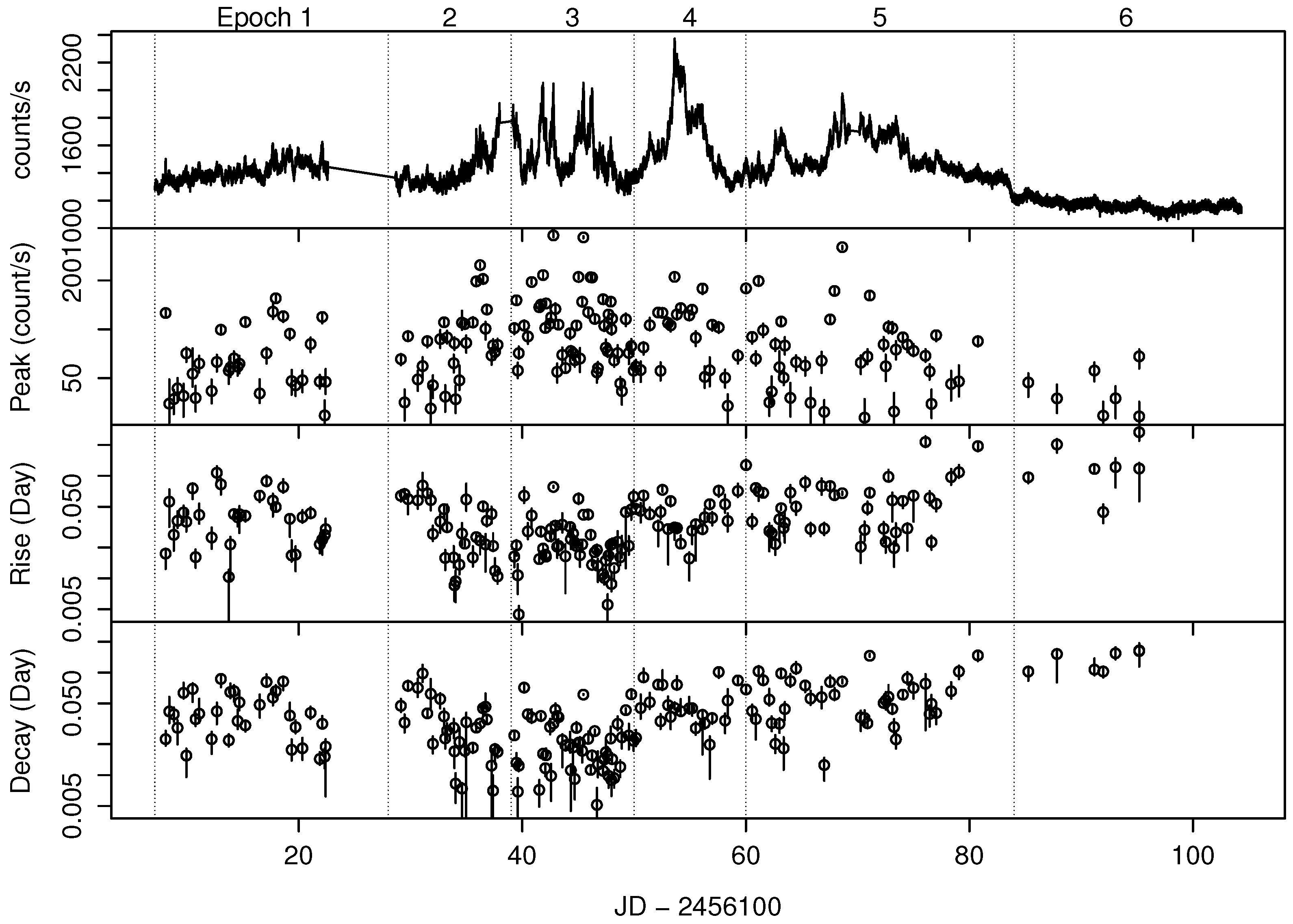
The upper panel of Figure 1 shows the optical light curve of the object obtained by Kepler. The blazar displayed violent variability over various timescales ranging from several tens of minutes to over 10 days during this monitoring. The light curve is composed of not only large-amplitude, long-term variations such as that ranging from JD 2456150 to 2456160, but also numerous flare-like variations with timescales less than one day. These rapid variations exist throughout this entire monitoring period. These variations have a wide variety of profiles.

3. Temporal Variation of Micro-Variation Profile

Blazar variability seems to consist of a number of components with various timescales that combine to form a continuous power-law PSD. We can extract the short-timescale variations from the rapid-cadence light curve over a short time range by approximating that the long-term component is constant over this time interval.

To study blazar microvariability, we parameterize the profile of the flux variations by the timescales during the rise and decay phases and the amplitudes of the micro-variation episodes. We define the procedure of parameter estimation as follows:

• Select a candidate micro-variation event
• Set a fitting time range to estimate the long-term component underlying the candidate event
• Estimate the best-fit second or third-order polynomial function for the long-term component
• Subtract this best-fit function over the fitting time range
• Identify the point of maximum flux as the peak date
• Estimate the amplitude at the peak (average 5 flux points around the peak to ignore the influence of fluctuations caused by statistical noise)
• Doubling times of the rise and decay phases are defined as the rise and decay timescales.

Figure 1 shows the light curve, time series of the amplitude, and the doubling times of the rise and decay phases in the detected micro-variation events. Averages and standard deviations of peak amplitudes, doubling times of rise and decay are 90 and 55 counts·s${}^{-1}$, 0.043 and 0.036 days, and 0.042 and 0.032 days, respectively. Typical uncertainties of parameters of 8 counts·s${}^{-1}$, 0.008 and 0.008 days are estimated from the uncertainty of the polynomial function by using a parametric bootstrap approach. The parameters representing the variation profiles vary with time. The variations of the rise and decay timescales behave almost the same. The rise and decay timescales of the events change not only randomly but also systematically. This result indicates that the events are associated with, rather than independent of, each other. 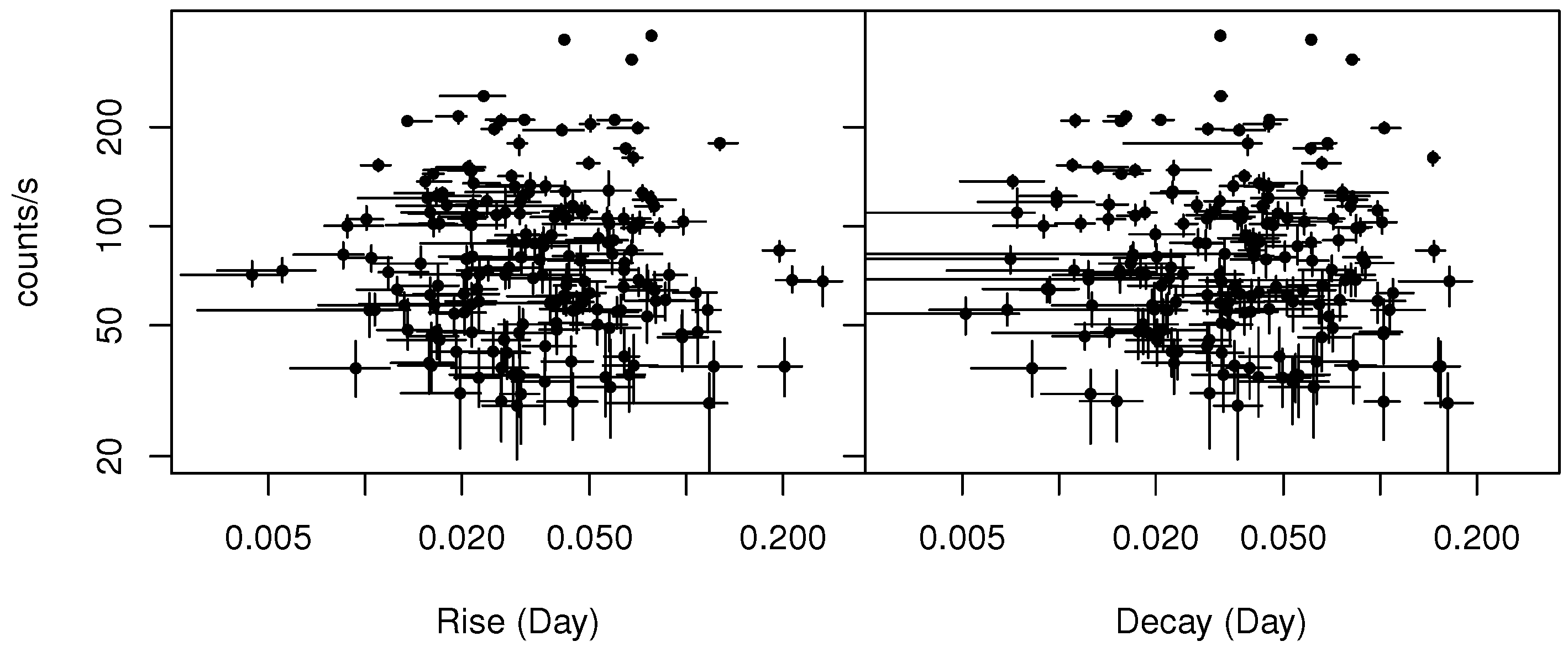Figure 2 shows correlations between peak amplitudes and rise and decay times. There are no clear correlations between the amplitudes and timescales.

4. Time Variation of Variability Timescales in Microvariations and Power Spectrum Density

Recent studies have reported that W2R 1926+42 has a characteristic timescale associated with a break frequency in the PSD of the object. The PSD, $P\left(f\right)$, calculated from the Kepler light curve is represented by a power-law plus a squared Lorentzian function with a constant value for the white noise as:

$$\begin{array}{c}\hfill P_{\mathrm{model}}\left(f\right)=A{f}^{-\alpha }+\frac{B}{{[1+{(f/f_{\mathrm{br}})}^2]}^2}+C,\end{array}$$

(1)

where α is a spectral index and $f_{\mathrm{br}}$ is a break frequency. The squared Lorentzian function corresponds to the exponential rise and decay pulse shape, because the pulse is Fourier-transformed to the squared Lorentzian function. Here, we assume that the shapes of microvariations with a characteristic timescale can be described as exponential pulses. We can estimate the e-folding time of such a pulse as the characteristic timescale corresponding to the break frequency of the squared Lorentzian function. The characteristic timescale estimated from the best-fit function of Equation (1) representing the PSD of the entire light curve is coincident with the e-folding time of the mean profile of 195 micro-variation events detected in the observed light curve (see [17] for more details). We study the time variation of the characteristic timescales estimated from the PSDs in each epoch of the light curve, and compare these characteristic timescales with the doubling times of the rise and decay phases in the micro-variation events.

We study the time evolution of the characteristic timescales that correspond to the break frequency of the PSD, and compare these timescales with the profile parameters of the micro-variation events. The PSDs are calculated from 6 epochs separating the observed light curve (from epoch 1 to 6; JD 2456107–2456123, 2456128–2456138, 2456139–2456150, 2456150–2456160, 2456160–2456184, 2456184–2456204). The best-fit values of the break frequency and corresponding timescale are estimated from the calculated PSDs.

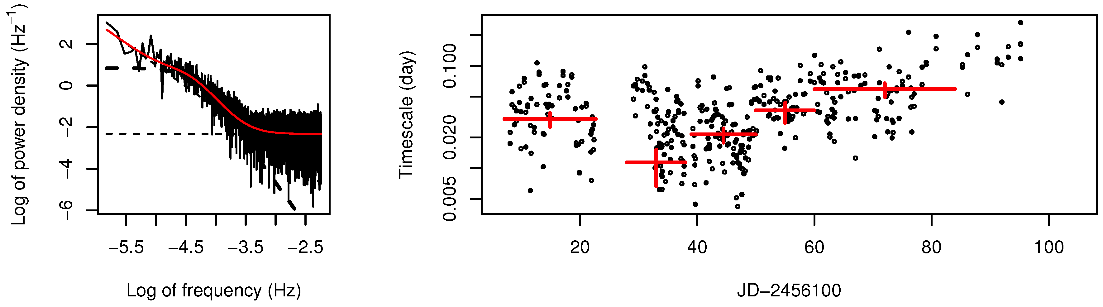
The left panel of Figure 3 shows an example of the PSD calculated from epoch 1 and its best-fit function from Equation (1). There is a break at 10${}^{-4.5}$ Hz in the PSD calculated from the light curve of epoch 1. The break frequency $f_{\mathrm{br}}$ corresponds to the characteristic e-folding timescale: ${\tau }_{\mathrm{br}}={\left(2\pi f_{\mathrm{br}}\right)}^{-1}$ [18]. The doubling timescale corresponds to $\left(\ln 2\right){\tau }_{\mathrm{br}}$. The break frequencies and corresponding characteristic timescales of the PSDs calculated from epoch 1 to 5 are estimated. The right panel of Figure 3 shows the time series of the characteristic timescales estimated from each PSD together with the doubling timescales during the rise and decay phases in the detected micro-variation events. The curvature is not seen in the PSD of epoch 6; we therefore cannot estimate its break frequency and characteristic timescale. There are differences between the estimated characteristic timescales at over 2σ confidence level, and, thus, the timescales vary over time. The estimated timescales tend to correlate with the doubling timescales of the detected micro-variation events. This indicates that the curvature of the PSD is caused by the rise and decay timescales of the microvariation.

5. Discussion

The doubling timescales of the detected microvariations change both randomly and systematically over time. If the flux variation is caused by changes in the high-energy particle acceleration of electrons or in the relativistic bulk motion, these accelerating events should be associated with each other, causing a systematic change of variation timescales. Several models have been proposed for the mechanisms of particle acceleration in blazar jets, for example, the shock-in-jet scenario [19] and magnetic reconnections [20]. Particle acceleration events are, however, expected to occur randomly in the basic versions of these proposed models. A particle acceleration event provided by a shock wave can arise from a supersonic collision of two plasmas. Similarly, particle acceleration via reconnection can occur in a plasma containing adjacent magnetic field lines of opposite polarity. These shocks or reconnection events are not associated with each other. Thus, flares caused by such unrelated particle acceleration events should, in general, arise independently.

The variation timescale of blazar variability $t_{\mathrm{obs}}$ is obtained by multiplying the rest-frame timescale $t_{\mathrm{jet}}$ by the Doppler factor $\delta ={(\mathrm{\Gamma }-\sqrt{{\mathrm{\Gamma }}^2-1}\cos \theta )}^{-1}$, $t_{\mathrm{jet}}=\delta t_{\mathrm{obs}}$, where Γ is the bulk Lorentz factor and θ is the inclination angle between the jet axis and our line of sight. Here, particle acceleration events occur in the jet flow.

Recently, several papers suggest that the particle acceleration can occur in regions that are moving relative to the main jet flow of blazars: turbulence [21] or reconnection “mini-jets” [20,22]. Emission from the accelerated particles is Doppler boosted by a Doppler factor computed from the superposed velocities of the mini-jet or turbulent cell and systemic jet flows. If a flare arises in such a region arising particle acceleration, the velocity and Doppler factor should be constant during the event, although the velocity of each event would be different. The peculiar velocities of the region affects the random aspect of variation timescales, not the systematic behavior, because the speeds and angles of relative motion can be random in the jet rest frame. The local active region moves down the jet, which may be bent (e.g., by pressure gradients and/or precession or wobbling of the jet axis) and may accelerate or decelerate. The systematic behavior of the variation timescales of microvariations can be explained by such global changes encountered by all emission regions that propagate down the jet.

6. Conclusions

The blazar W2R 1926+42 exhibits violent variability with timescales less than one day, which is known as microvariability. We have detected 195 micro-variation events from a continuous optical light curve with 1-min time resolution obtained by the Kepler spacecraft. Estimated variation timescales of microvariability events varied both randomly and systematically with time. Furthermore, the variation timescales are associated with characteristic timescales estimated from break frequencies of power spectrum densities calculated from 6 epochs into which we divide the light curve that we have obtained. Such systematic changes of variation timescales imply that the particle acceleration events are mutually correlated by common physical influences such as bends in the jet flow. On the other hand, random behavior on intra-day timescales can be associated with variations caused by changes in the peculiar velocities (relative to the systemic flow) of local emission regions.

References

- Antonucci, R. Unified models for active galactic nuclei and quasars. Annu. Rev. Astron. Astrophys. 1993, 31, 473–521. [Google Scholar] [CrossRef]
- Blandford, R.D.; Königl, A. Relativistic jets as compact radio sources. Astrophys. J. 1979, 232, 34–48. [Google Scholar] [CrossRef]
- Kataoka, J.; Takahashi, T.; Wagner, S.J.; Iyomoto, N.; Edwards, P.G.; Hayashida, K.; Inoue, S.; Madejski, G.M.; Takahara, F.; Tanihata, C.; et al. Characteristic X-Ray Variability of TeV Blazars: Probing the Link between the Jet and the Central Engine. Astrophys. J. 2001, 560, 659–674. [Google Scholar] [CrossRef]
- Quirrenbach, A.; Witzel, A.; Kirchbaum, T.P.; Hummel, C.A.; Wegner, R.; Schalinski, C.J.; Ott, M.; Alberdi, A.; Rioja, M. Statistics of intraday variability in extragalactic radio sources. Astron. Astrophys. 1992, 258, 279–284. [Google Scholar]
- Carini, M.; Miller, H.R.; Goodrich, B.D. The timescales of the optical variability of blazars. I-OQ 530. Astron. J. 1990, 100, 347–356. [Google Scholar] [CrossRef]
- Sasada, M.; Uemura, M.; Arai, A.; Fukazawa, Y.; Kawabata, K.S.; Ohsugi, T.; Yamashita, T.; Isogai, M.; Sato, S.; Kino, M. Detection of Polarimetric Variations Associated with the Shortest Time-Scale Variability in S5 0716+714. Publ. Astron. Soc. Jpn. 2008, 60, L37–L41. [Google Scholar] [CrossRef]
- Aharonian, F.; Akhperjanian, A.; Bazer-Bachi, A.; Behera, B.; Beilicke, M.; Benbow, W.; Berge, D.; Bernlohr, K.; Boisson, C.; Bolz, O.; et al. An Exceptional Very High Energy Gamma-Ray Flare of PKS 2155–304. Astrophys. J. 2007, 664, L71–L74. [Google Scholar] [CrossRef]
- Abdo, A.A.; Ackermann, M.; Ajello, M.; Allafort, A.; Baldini, L.; Ballet, J.; Barbiellini, G.; Bastieri, D.; Bellazzini, R.; Berenji, B.; et al. Fermi Gamma-ray Space Telescope Observations of the Gamma-ray Outburst from 3C454.3 in November 2010. Astrophys. J. 2011, 733, L26–L33. [Google Scholar] [CrossRef]
- Saito, S.; Stawarz, Ł.; Tanaka, Y.T.; Takahashi, T.; Madejski, G.; D’Ammando, F. Very Rapid High-amplitude Gamma-Ray Variability in Luminous Blazar PKS 1510–089 Studied with Fermi-LAT. Astrophys. J. 2013, 766, L11–L17. [Google Scholar] [CrossRef]
- Nalewajko, K. The brightest gamma-ray flares of blazars. Mon. Not. R. Astron. Soc. 2013, 430, 1324–1333. [Google Scholar] [CrossRef]
- Edelson, R.; Malkan, M. Reliable Identifications of Active Galactic Nuclei from the WISE, 2MASS, and ROSAT All-Sky Surveys. Astrophys. J. 2012, 751, 52–64. [Google Scholar] [CrossRef]
- Edelson, R.; Mushotzky, R.; Vaughan, S.; Scargle, J.; Gandhi, P.; Malkan, M.; Baumgartner, W. Kepler Observations of Rapid Optical Variability in the BL Lacertae Object W2R1926+42. Astrophys. J. 2013, 766, 16–24. [Google Scholar] [CrossRef]
- Borucki, W.J.; Koch, D.; Basri, G.; Batalha, N.; Brown, T.; Caldwell, D.; Caldwell, J.; Christensen-Dalsgaard, J.; Cochran, W.D.; DeVore, E.; et al. Kepler Planet-Detection Mission: Introduction and First Results. Science 2010, 327, 977–980. [Google Scholar] [CrossRef] [PubMed]
- Jenkins, J.M.; Caldwell, D.A.; Chandrasekaran, H.; Twicken, J.D.; Bryson, S.T.; Quintana, E.V.; Clarke, B.D.; Li, J.; Allen, C.; Tenenbaum, P.; et al. Overview of the Kepler Science Processing Pipeline. Astrophys. J. 2010, 713, L87–L91. [Google Scholar] [CrossRef]
- Koch, D.G.; Borucki, W.J.; Basri, G.; Batalha, N.M.; Brown, T.M.; Caldwell, D.; Christensen-Dalsgaard, J.; Cochran, W.D.; DeVore, E.; Dunham, E.W.; et al. Kepler Mission Design, Realized Photometric Performance, and Early Science. Astrophys. J. 2010, 713, L79–L86. [Google Scholar] [CrossRef]
- Van Cleve, J.; Caldwell, D. Kepler Instrument Handbook, KSCI-10933-001; NASA Ames Research Center: Mountain View, CA, USA, 2010. [Google Scholar]
- Sasada, M.; Mineshige, S.; Yamada, S.; Negoro, H. Understanding the General Feature of Microvariability in Kepler Blazar W2R 1926+42. Publ. Astron. Soc. Jpn. 2017, 69, 15. [Google Scholar] [CrossRef]
- Negoro, H.; Kitamoto, S.; Mineshige, S. Temporal and Spectral Variations of the Superposed Shot as Causes of Power Spectral Densities and Hard X-Ray Time Lags of Cygnus X-1. Astrophys. J. 2001, 554, 528–533. [Google Scholar] [CrossRef]
- Marscher, A.P.; Gear, W.K. Models for high-frequency radio outbursts in extragalactic sources, with application to the early 1983 millimeter-to-infrared flare of 3C 273. Astrophys. J. 1985, 298, 114–127. [Google Scholar] [CrossRef]
- Giannios, D.; Uzdensky, D.A.; Begelman, M.C. Fast TeV variability in blazars: jets in a jet. Mon. Not. R. Astron. Soc. 2009, 395, L29–L33. [Google Scholar] [CrossRef]
- Marscher, A.P. Turbulent, Extreme Multi-zone Model for Simulating Flux and Polarization Variability in Blazars. Astrophys. J. 2014, 780, 87–97. [Google Scholar] [CrossRef]
- Nalewajko, K.; Giannios, D.; Begelman, M.C.; Uzdensky, D.A.; Sikora, M. Radiative properties of reconnection-powered minijets in blazars. Mon. Not. R. Astron. Soc. 2011, 413, 333–346. [Google Scholar] [CrossRef]
© 2017 by the authors. Licensee MDPI, Basel, Switzerland. This article is an open access article distributed under the terms and conditions of the Creative Commons Attribution (CC BY) license ( http://creativecommons.org/licenses/by/4.0/).