1. Introduction
A few years after Einstein’s epic proposal of the general theory of relativity, there was an attempt to formulate an alternative theory without the methodological complications of general relativity concerning the modification of spacetime geometry. This theory was developed by A. N. Whitehead, best known for his work in philosophy, in a book entitled
The Principle of Relativity [
1,
2]. Whitehead was interested in preserving the underlying Minkowski geometry as the real structure of spacetime, while gravitation was understood as a symmetric covariant tensor
,
μ,
, which is not related to spacetime’s topology, but is invariant under the Poincaré group.
The effect of this tensor field manifests itself through the equations of motion of test particles defined in terms of the geodesic lines generated by the Christoffel symbols associated with the tensor
. To build his proposal for the field tensor, Whitehead begins defining the null vector:
where
are the spacetime coordinates of the test particle and
are the coordinates of the intersection of the past cone corresponding to the event
and the world-line,
W, of the point-like source. If
is the fourth velocity along this world-line, we also define the scalar
r and the reduced null vector
as follows:
Whitehead’s proposal is not a proper field theory, but instead, it is entirely based on the following symmetric covariant tensor:
where
is the diagonal Minkowski metric:
,
,
,
. For a point-like mass source at rest, the tensor
is given by:
Eddington noticed that this metric can be transformed into the standard Schwarzschild metric with coordinates
by the transformation:
Moreover, Russell and Wassermann [
3,
4] showed that the Kerr solution for a rotating black hole is of Whitehead’s form when expressed in terms of advanced null coordinates. This is not strange, because the tensor in Equation (
3) is written in the Kerr–Schild form [
5]. A consequence of this mathematical similarity is that Whitehead’s theory makes the same predictions as Einstein’s GR for the so-called classical tests: the bending of stellar light rays grazing the surface of the Sun, the anomalous advance of Mercury’s perihelion and gravitational redshift [
2]. On the other hand, Shapiro’s echo delay [
6] and the most recent test for the geodetical and gravitomagnetic precession of orbiting superconducting gyroscopes transported by the Gravity Probe B [
7,
8] are also in agreement with Whitehead’s theory, as well as GR [
10].
For all of these reasons, Whitehead’s theory has been greatly valued for many decades after its formulation in 1922 [
2,
11,
12]. Thirty years later, a series of lectures was given by Synge, who still recognized this alternative as a serious contender to GR as the fundamental theory of gravity [
2]. However, other authors showed later on that anti-damping of binary pulsars' orbits is also predicted in contrast to the
damping effect of GR due to the radiation of gravitational waves. The GR prediction was proven right, beyond any doubt, in the careful observations of the pulsar B1913+16 by Hulse and Taylor [
9,
10]. Anisotropy in the gravitational constant, violations of the weak equivalence principle and Birkhoff’s theorem have also been invoked as irrecoverable inconsistencies with experience in Whitehead’s model [
10].
Being a linear model, it is not surprising that incorrect predictions arise when applied to strong fields, but there are still reasons to study it, because some important phenomena not contemplated by GR could be revealed at this level. For example, Coleman suggested that a distortion of the Coulomb potential near the mass of the Sun, predicted by Whitehead’s theory, could explain the, still unexplained, Limb effect (the difference between the redshift of a line emitted at the center of the solar disk and the average of the redshift of lines emitted at the east and west sides of the solar disk) [
2,
14,
15].
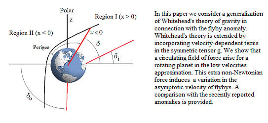
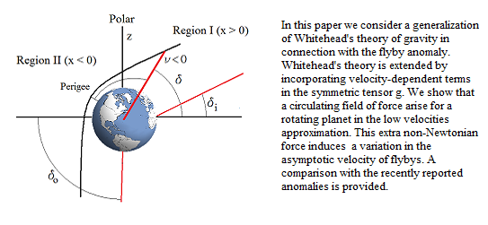
In this paper, we consider an extension of Whitehead’s theory in terms of the more general Poincaré invariant tensor,
, including the
vector and the fourth velocity of the source,
. The objective of this paper is to show that this extended theory predicts an anomalous variation in the velocity of a spacecraft flying by the Earth. This is to be compared, in sign and order of magnitude, to the recently-reported anomalous orbital-energy changes in several gravity assist maneuvers involving flybys of the Earth [
16,
17].
2. The Extended Whitehead Theory
In this section, we briefly review the proposal of an extended Whitehead formalism as given by Bel [
22,
23]. Firstly, we define the fourth velocity
for a point source moving in a Galilean frame of reference,
. A particular event in the trajectory of the source is denoted by
, while an event in the future of
, where we want to calculate the gravitational field, is denoted by
. By using all possible combinations of
as defined in Equation (
2) and the fourth velocity,
, we arrive at the following expression for the symmetric tensor
:
where
denotes Minkowski’s metric as usual and
,...,
are constants to be determined in order to agree with observations. In the first place, the condition imposed by Einstein’s vacuum equations,
, can be used to find the relation
. Consistency with the Newtonian limit also implies that
,
G being the gravitational constant and
m the mass of the source.
The equations of motion are given in terms of the Christoffel symbols:
where
τ is the proper time,
is the fourth velocity of the test particle and
are the Christoffel symbols in the linear approximation:
where the hat superscript denotes Synge’s derivatives defined as follows:
If the spatial components of the velocities are small compared to the speed of light, we have the following simplification (as deduced by Bel [
23]):
where
and
,
,
are, respectively, the spatial components of the velocity of the test particle and the source. We now consider two cases: a source moving with uniform velocity and a uniformly rotating source. We are going to see that only in the second case (corresponding to rotational acceleration), effects different from the Newtonian prediction are found.
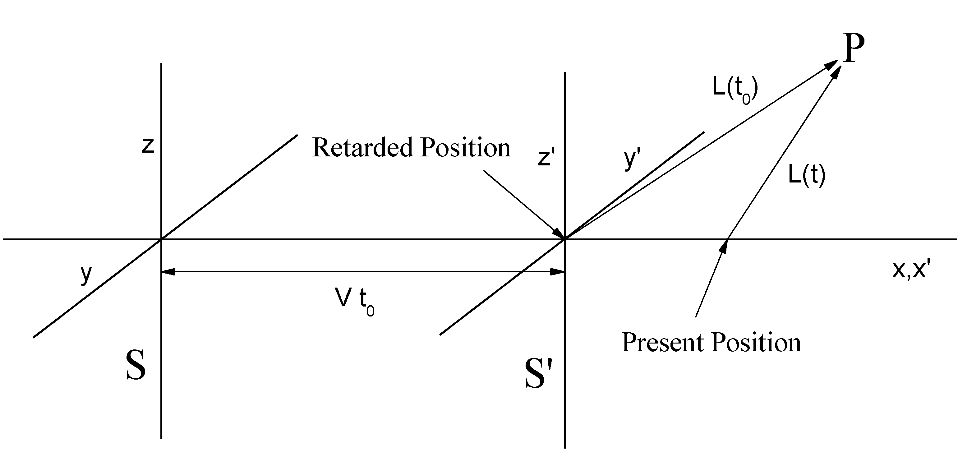
2.1. A Source Moving at Constant Speed
We consider a point-like source moving at constant speed
V along the
x axis of an inertial system of reference,
S. The location of the source at time
is
,
, as shown in
Figure 1. We are interested in calculating the gravitational acceleration induced upon a test particle located at point
P at time
t, with coordinates
x,
y,
z.
The velocity of the test particle is given by
,
. We can now use Equation (
12) to calculate (to first order in
) the acceleration of a test particle located at
P at time
t. A straightforward calculation of the retarded terms yields:
where we have ignored terms
and the relation among the retarded and present distances has been used:
Therefore, from Equations (
13)–(15), we deduce that the gravitational forces exerted upon the test particle in point P apparently emanate from the present position of the source as it would happen in Newton’s theory of action at a distance. This was already pointed out (in the context of a Lorentz-invariant model of gravity) by Poincaré [
18]. Aberration is also absent in general relativity up to order
[
21]. In the next section, we see that, in the case of accelerating sources, extra non-Newtonian forces appear.
Figure 1.
Two inertial systems of reference: S and . The source is at the origin of , which moves at constant speed V in the x direction with respect to S. is the retarded path to the test particle at P, and is the distance from the present position of the source at the time t (we are interested in measuring the gravitational force at this time, t).
2.2. The Uniformly-Rotating Source
The velocity of an element of mass at a distance
r from the center of a rotating planet can be written as follows:
ω being the rotational angular velocity of the planet. Here, the third axis corresponds to the rotation axis of the planet. We have also that:
where
D denotes the distance of the test particle from the center of the planet. By integrating
in Equation (
12) over the whole volume of the planet, assumed of uniform density, we obtain the following components of the force acting upon the test particle [
23]:
where
δ is the declination of the test particle. Notice that Equations (
19) and (21) correspond to the standard Newtonian force, but Equation (20) is an extra force term perpendicular to the planes of constant right ascension. In the next section, we will show that this non-Newtonian term gives rise to an anomalous variation of the asymptotic flyby velocities of the same order of magnitude as those studied by Anderson
et al. [
16].
We must also take into account that the approximation in Equation (20) is only good for
, and it can become quite crude when the spacecraft is close to the perigee. In this region, the integration over the mass elements of the Earth (considered of uniform density) must be calculated numerically. The expression for the non-Newtonian force is then given by:
where
and:
with:
In
Section 4, we will compare the results of the simplified perturbing force in Equation (20) and the exact one in Equation (
22) obtained by numerical integration.
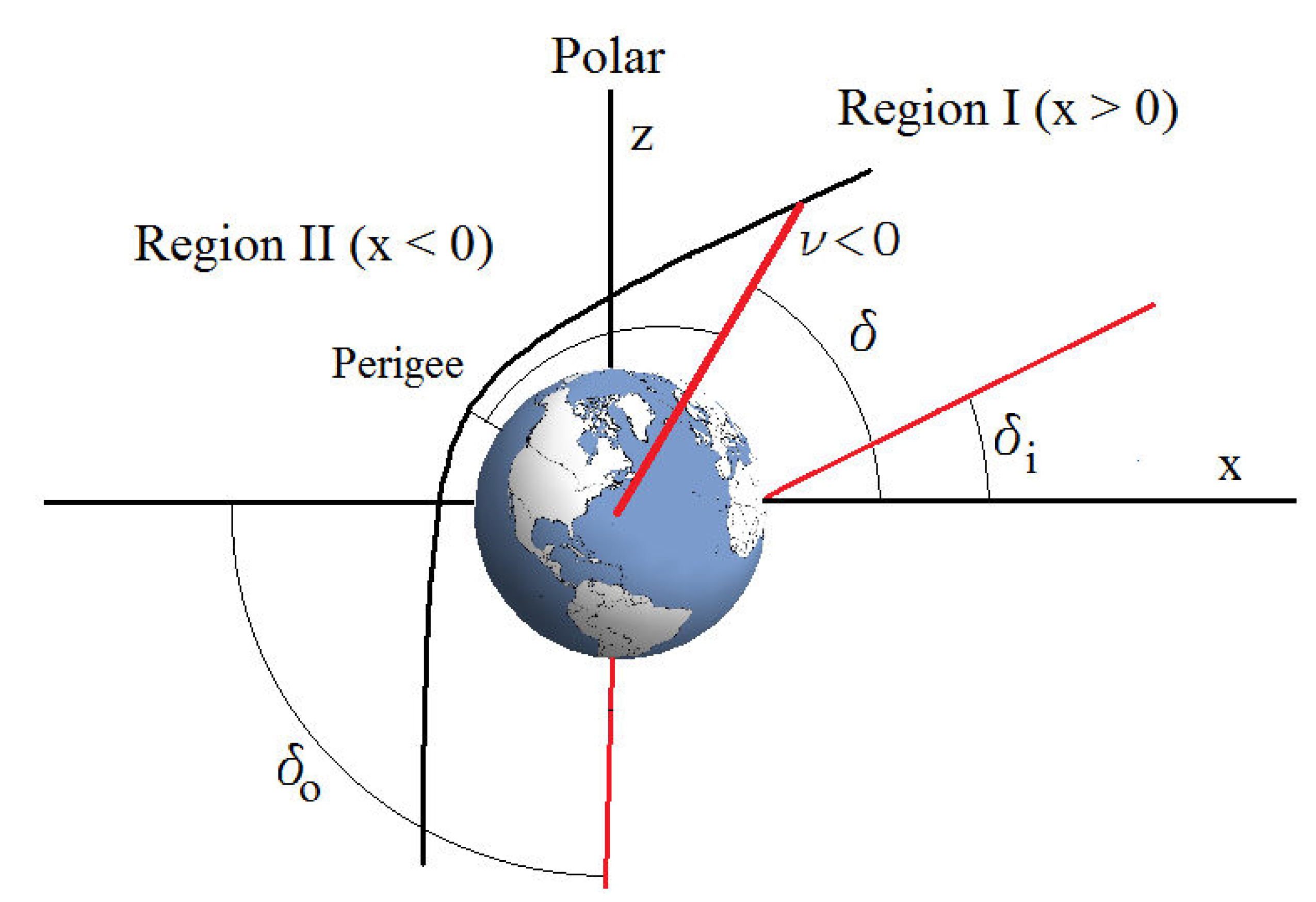
3. Idealized Polar Flyby
In this section, we consider an idealized polar flyby in which the trajectory of the spacecraft is confined to a plane perpendicular to the equator and containing the center of the Earth. For this particular orbit, the calculations can be performed explicitly, and it can, approximately, be applied to the NEAR flyby of 23 January 1998. This ideal trajectory is plotted in
Figure 2.
Figure 2.
An ideal flyby in a plane with constant right ascension, α. The true anomaly is denoted by ν; ϕ is the perigee’s latitude, and , are the declinations for the incoming and outgoing directions, respectively. The Region I() corresponds to the section of the orbit with, , where is the true anomaly of the orbital point located just in the rotation axis of the Earth.
We now consider a perturbing force of the form mentioned in the previous section for
:
where
,
M being the mass of Earth and
R its radius. We have also used the polar angle for convenience, because, in this ideal orbit, the polar angle,
θ, and the declination,
δ, are complementary,
. The perturbing force in Equation (
25) is a circulating vector field that follows the celestial parallels,
i.e., the sign of the component
changes when we consider the reversal of the
x,
y coordinates in the Earth’s equatorial plane.
The impulse imparted to the spacecraft by this non-Newtonian gravitational interaction yields the total variation of the velocity vector:
where
F denotes the perturbing force. To perform this integral, it is useful to recall some useful relations in celestial mechanics [
19,
20]:
where
u is the eccentric anomaly,
ν is the true anomaly,
ϵ is the orbital eccentricity and
is the characteristic timescale of the hyperbolic Keplerian orbit. The distance from the spacecraft to the center of the Earth can also be written as follows:
with
denoting the semi-major axis. We must also take into account that the polar angle,
θ, is related to the true anomaly,
ν, by different expressions in Region
I (
) and Region
(
):
By using Equations (
25)–(
29), we deduce the variation of the component of the spacecraft’s velocity normal to the osculating plane arising from the perturbing force in Equation (
25):
in which the prefactor can also be simplified to:
The explicit evaluation of the integral in Equation (
30) finally yields:
where:
Notice that the incoming and outgoing true anomalies can be obtained in terms of the declinations of the initial and final directions of the spacecraft and the latitude of the perigee:
The phenomenological fitting suggested by Anderson
et al. [
16] for the anomalous perturbation in the asymptotic velocity of the spacecraft flying by the Earth can be written as follows:
The prefactor in Equation (
35) is of the same order of magnitude as the one in Equation (
32), because for flybys grazing the Earth, the semi-major axis is not very different from the Earth’s radius. Another interesting feature of Equation (
33) is that it becomes null for a symmetric flyby over the poles corresponding to
,
. This is also predicted by Anderson’s phenomenological formula.
The ratio of the Earth’s equatorial velocity and the speed of light is
. The parameters for the NEAR and other flybys are listed in
Table 1. Using Equations (
29), (
32) and (
33) with these parameters for NEAR, we get
mm/s,
i.e, approximately 10% of the observed value amounting to
mm/s, which, on the other hand, is fitted well by Anderson’s formula in Equation (
35).
Table 1.
Parameters for the spacecraft flybys of the Earth: date corresponding to the perigee, eccentricity (ϵ), semi-major axis (a), polar angle for the incoming () and outgoing () directions, polar angle for the perigee (), velocity at closest approach, , right ascension for the perigee () and orbital inclination, I.
| Spacecraft | Date | ϵ | a (km) | | | | (km/s) | | I |
|---|
| NEAR | 1/23/1998 | 1.8135 | -8494.87 | 69.24° | 161.96° | 57° | 12.74 | 358.25° | 108° |
| Galileo I | 12/8/1990 | 2.4729 | -4977.24 | 77.48° | 124.25° | 64.8° | 13.74 | 11.48° | 142.9° |
| Galileo II | 12/8/1992 | 2.3194 | -5058.31 | 55.74° | 94.87° | 123.8° | 14.08 | 77.56° | 138.7° |
| Cassini | 8/18/1999 | 5.8525 | -1555.09 | 102.92° | 94.99° | 113.5° | 19.03 | 221.90° | 25.4° |
| Rosetta | 3/4/2005 | 1.3118 | -26,710.9 | 92.8° | 124.29° | 69.8° | 10.52 | 324.28° | 144.9° |
| Messenger | 8/2/2005 | 1.3606 | -24,174.8 | 121.44° | 121.92° | 43.08° | 10.34 | 347.94° | 133.05° |
| Juno | 9/10/2013 | 4.6489 | -3645.92 | 104.21° | 50.59° | 123.39° | 13.01 | 291.85° | 47.13° |
4. Numerical Integration and Perturbations on Closed Orbits.
For the rest of the flybys, we can obtain the asymptotic perturbations in the outgoing velocity with respect to the ingoing velocity of the spacecraft by performing a numerical integration. We will also consider both the approximation for
in Equation (20) and the exact result in Equations (
22)–(
24).
As has already been discussed in previous works [
24], it is convenient to define a Cartesian system of reference anchored to the Earth in which the
z axis is the rotation axis of the planet,
x is directed towards the point of Aries (defined by the intersection of the ecliptic and equatorial planes) and
y is finally chosen to form a right-handed system.
We also define the non-dimensional time
, radio vector
and velocity
. The perturbations in the spacecraft position and velocity are then obtained by solving the following equations of motion:
where
is the anomalous acceleration imparted by the extra effect predicted by the extended Whitehead theory as given in Equation (
25) and
is the perturbation in the Newtonian acceleration imparted by the Earth as a consequence of the deviation of the trajectory from the Keplerian hyperbolic orbit [
24]. Integrations are performed by using the eccentric anomaly variable, which runs from
to
during the flyby. The distance to the center of the Earth is then expressed as in Equation (
28), and the polar angle can be calculated as:
where
r is the orbital radio vector of the spacecraft. We can approximate
r by the position in the ideal hyperbolic orbit:
where
u is the eccentric anomaly,
is a unit vector pointing from the center of the Earth towards the perigee and
is another unit vector in the osculating plane of the orbit at perigee, normal to
and pointing towards the incoming direction of the flyby [
24].
From Equations (
25) and (
36), we can write explicitly the system of equations that we have used to integrate the motion of the spacecraft:
where
D is the radio vector of the spacecraft from the center of the Earth (in units of the semi-major axis,
) for the unperturbed Keplerian orbit as given in Equation (
38). Instead of the scaled time,
τ, we use the eccentric anomaly,
u, as the integration variable. The relation among these two variables is given by:
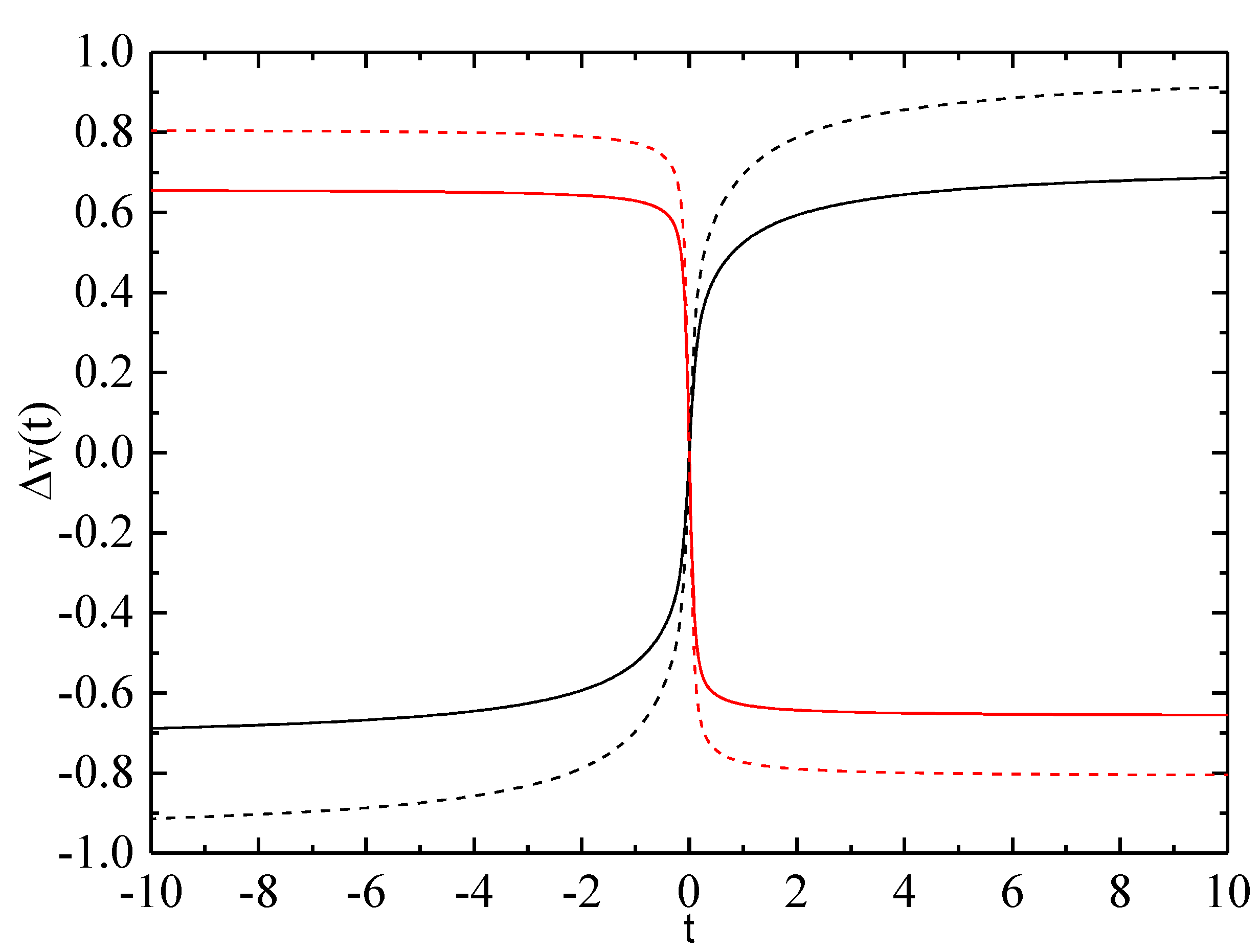
In
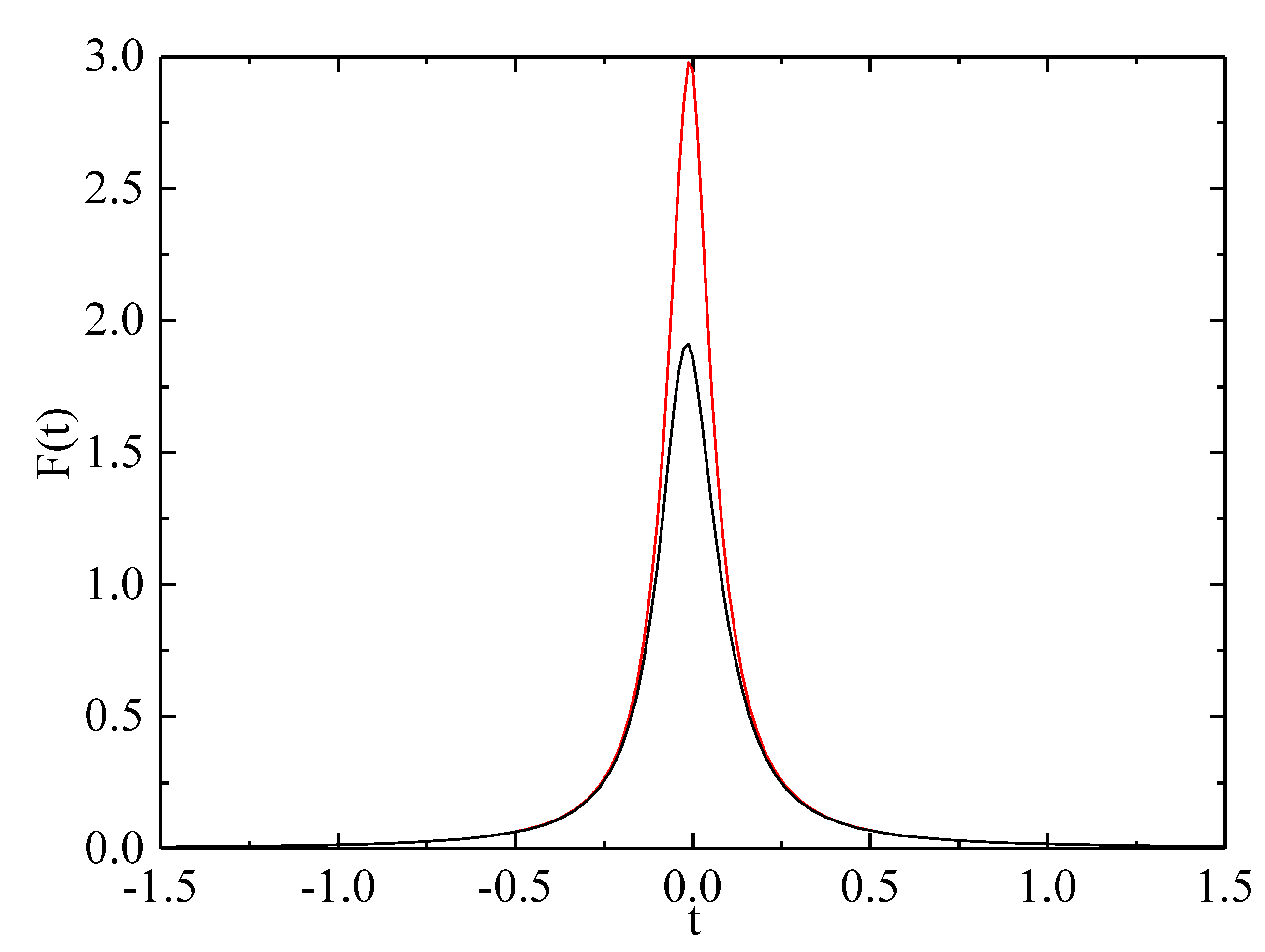
Figure 3, we have plotted the results for the NEAR and Cassini flybys. In the case of the NEAR flyby, a small increase of
mm/s is obtained, and for the Cassini flyby, we have a decrease of
mm/s in the interval running from
to
, which corresponds to
hours before and after the flyby for NEAR and
hours for Cassini. If we use the force integral in Equation (
22), we find the values
mm/s and
mm/s for NEAR and Cassini, respectively. The results in
Figure 3 for the anomalous variation of the velocity modulus are expressed in terms of time,
t, in hours. Notice that most of the variation is taking place two hours before and after the instant of closest approach.
Figure 3.
Perturbation in the modulus of the orbital velocity (in mm/s) as a consequence of the force term in Equation (
25)
vs. time (in hours). The black and red lines correspond to the NEAR and Cassini flybys, respectively. Dashed lines correspond to the integration using the exact expression of the force in Equation (
22). The perigee (
) has been taken as the reference to determine the osculating plane containing the ideal Keplerian orbit.
In
Table 2, we compare the predictions of the model (from Equations (
25) and (
22)) with the values deduced from the analysis of Doppler residuals and the fitting obtained by Anderson
et al. [
16]. In
Figure 4, we compare the scaled perturbing force, normalized with the factor
, for the rigorous expression in Equation (
22) and the approximation of Equation (
25) for the Cassini flyby. As this spacecraft reached its perigee only at 303 km from Earth’s surface, we see that the approximation
is quite crude. However, the impact on the total perturbation is not very noticeable.
Table 2.
Observed increments/decrements of the asymptotic velocity of several spacecraft during flybys of the Earth (first column) compared to the prediction of Anderson’s formula in Equation (
35) and the result of the extended Whitehead theory.
Table 2.
Observed increments/decrements of the asymptotic velocity of several spacecraft during flybys of the Earth (first column) compared to the prediction of Anderson’s formula in Equation (35) and the result of the extended Whitehead theory.
| Spacecraft | | | Equation (25) | Equation (22) |
|---|
| NEAR | 13.46 | 13.28 | 1.454 | 1.922 |
| Galileo I | 3.92 | 4.12 | 2.389 | 3.015 |
| Galileo II | -4.6 | -4.67 | 2.741 | 3.815 |
| Cassini | -2 | -1.07 | -1.317 | -1.615 |
| Rosetta | 1.80 | 2.07 | 5.187 | 6.046 |
| Messenger | 0.02 | 0.06 | 3.701 | 4.236 |
| Juno | not reported yet | 6.38 | -0.497 | -0.523 |
The agreement is reasonable in the case of the Cassini and Galileo II flybys, but is far too small for NEAR. However, from a theoretical standpoint, it is remarkable that such an effect can be derived from minimum premises as those assumed in Whitehead’s theory [
2] and the extension by Bel [
22,
23].
Figure 4.
Scaled perturbing forces for the Cassini flyby. The red line corresponds to the predictions of Equation (
22) and the black line to those of Equation (
25). Notice that there is a remarkable difference at the perigee,
Figure 4.
Scaled perturbing forces for the Cassini flyby. The red line corresponds to the predictions of Equation (
22) and the black line to those of Equation (
25). Notice that there is a remarkable difference at the perigee,
We could also point out that, according to the perigee altitude,
h, flybys can be classified in two groups: (i) low-altitude flybys: Galileo I (
km), Galileo II (
km) and NEAR (
km); and (ii) high-altitude flybys: Cassini (
km), Rosetta (
km) and Messenger (
km). It is remarkable that the absolute value of the flyby anomaly is larger for the members of the first group [
16]. However, we have insufficient data to assess the statistical significance of this hypothesis. On the other hand, it seems that, if the flyby anomaly is the result of putative unknown interaction, this should decrease very quickly with the distance to the center of the Earth. The dipole-like interaction in Equation (
25) resulting from the extended Whitehead model exhibits a
dependence, which, apparently, conforms to this hypothesis, but the dependence of the perturbation induced by this perturbation on the orbital orientation cannot be ignored. On the other hand, the predictions listed in
Table 2 disagree with the
a priori classification, emphasizing the importance of orbital orientation for this particular interaction.
The problem with this model, and others proposed so far, is that the large magnitude of the flyby anomaly seems incompatible with our present knowledge of the Earth’s gravitational field derived from the motion of artificial satellites and the Moon. In the next section, we will show that, if the perturbation force field derived in Equation (
25) is also affecting the Moon’s motion, the result would be totally inconsistent with radar and laser ranging measurements.
4.1. Perturbations on the Moon’s Orbit
Although the results in the previous section seem promising, we must also check the effects upon circular orbits. For a tangential perturbing force, as given in Equation (
25), the variation of the semi-major axis is given by [
19,
20]:
where
is the tangential velocity and
T is the tangential component of the perturbing force. For the particular case of a circular orbit in the equatorial plane, we have:
where
R is the radius of the Earth,
ω is its angular velocity,
M is the mass of the Earth and
a is the orbital radius. In the Earth-Moon system, we have, approximately,
km
3/s
2,
km,
rad/s and
km. From these values, we deduce
m per year, which is clearly in disagreement with the observations. For a comparison with this large prediction for the variation of the Earth-Moon distance, it is known that tidal effects imply an average receding rate of the Moon from the Earth of
m per year [
25]. We conclude that this is an unrealistic prediction of the linear approximation in Equation (
8) despite any compatibility with the flyby anomaly observations.
5. Conclusions
The flyby anomaly is a lingering problem in astrodynamics since its first detection in the post-encounter radio data generated for the Galileo I flyby on 8 December 1990. Increments and decrements in the asymptotic velocity of spacecraft flying by the Earth have been found for many maneuvers of this kind in the last twenty five years. In 2008, Anderson
et al. [
16] proposed their empirical formula fitting the results for six flybys that have taken place in the period 1990–2005. This formula relates the ratio among the anomalous variation of the spacecraft’s velocity and the total asymptotic velocity with the linear velocity of the Earth’s equator divided by the speed of light and the variation of the cosine of the declination of the incoming and outgoing velocity vectors. Despite its simplicity, it fits reasonably well with the data known at the time.
Anderson’s formula is important because it may indicate that this anomaly has not a systematic origin, but it could be modeled by an unknown interaction. On the other hand, a theoretical substantiation of this claim is still lacking. Some recent unconventional proposals for a possible explanation of the anomaly include: a halo of dark matter around the Earth [
28], anomalous couplings to the gravitational potential vector of the linearized theory [
29] or a circulating gravitomagnetic field [
30]. Lämmerzahl
et al. [
31] considered several other conventional effects: atmospheric friction, ocean and solid tides, spacecraft charge, magnetic moment, Earth albedo, solar wind and spin-rotation coupling, but they were found insufficient to explain the anomaly. Iorio has also studied the effect of zonal harmonics at the Newtonian and post-Newtonian level, but their effects have also been found small to account for a variation of a few mm/s in the outgoing velocity with respect to the incoming velocity of the spacecraft [
32]. The same can be said of the gravitomagnetic and gravitoelectric effects in standard general relativity [
33].
A systematic or more subtle error in the analysis of the data for the flybys would be the easier explanation. However, if any computational error or conventional explanation is finally discarded, this creates a very fundamental problem in gravitational physics. The observed changes in energy referred to the system of reference of the Earth are really very large in the context of our present knowledge of gravitation in the solar system. This means that it is difficult to find an expression for a putative unknown interaction explaining the flyby anomaly without giving rise to non-observed perturbations in the bound orbits of artificial satellites or the Moon.
In this paper, we have considered a modified version of Whitehead’s theory, first introduced in 1922. In this theory, a transversal perturbing force appears in the proximity of a rotating planet, and we have shown that this force gives rise to an anomalous increase (or decrease, in certain cases) of the velocity of spacecraft flying by. The order of magnitude of this effect coincides with the observations, and the values and sign are similar in some cases (but not all). However, we also show that such a force extrapolated to the orbit of the Moon implies an extraordinarily large rate of variation for the semi-major axis. Consequently, we must conclude that extra forces, as that suggested in Equation (
25), are not compatible with all of the observations, including bound orbits. We must notice that such a hypothetical interaction should also be compatible with some, recently discovered, planetary anomalies [
17].
Nowadays, laser ranging allows for a very precise determination of the orbit of the Moon and that of the geodynamic satellites, such as LAGEOS and LARES [
34,
35,
36,
37,
38,
39]. With this powerful experimental tool, it has been shown that the Moon recedes from the Earth at a rate of 38 mm per year as a consequence of the tidal interaction with the Earth. Determination of the Lense–Thirring effect has even been possible by combining the data of the LAGEOS and LAGEOS II satellites [
40,
41]. Further insight will be surely obtained with the STE-QUEST mission [
42], specially dedicated to gravitation research, whose launch is projected for the next decade. This mission is particularly suited for probing the anomaly, because the satellite is intended to describe a highly eccentric orbit whose perigee will change from an altitude of 700 km to 2000 km, precisely in the range of the flybys analyzed so far.
The task and challenge for the near future is to find a model capable of fitting all of the data for the flyby anomaly without conflicting with the precise measurements for bound orbits. It seems that such extra force should have larger effects for highly eccentric orbits with low perigees. This is not the case for the predictions of the generalized Whitehead model discussed in this paper, but we have shown that a theoretical foundation of this paradoxical anomaly is possible.
Moreover, a clearly-defined consequence of the extended Whitehead model is a direct proportionality of the possible new interaction, causing the flyby anomaly, with the total angular momentum of the planet. In connection with this prediction, the Juno spacecraft is planned to be captured in a highly eccentric elliptic orbit around Jupiter in July 2016 (
). Some studies have shown that the standard Lense–Thirring and other effects predicted by general relativity are a possible result to be found [
43,
44,
45,
46,
47]. Juno’s orbital periapsis will be located at 6% of the planetary radius, and the apoapsis is expected to be reached at 20-times Jupiter’s radius. If we take into account that the rotational angular momentum of Jupiter is five orders of magnitude larger than that of the Earth, we are also at ideal conditions for studying the flyby anomaly. This data could prove essential for further understanding of this anomalous effect, and if the anomaly is detected, it surely will attract more interest to the problem. We hope that further alternatives will be explored in order to achieve the convergence of the theoretical and experimental approaches for the solution of this dilemma in gravitational physics.


