Assessing the Potential for Liquid Solvents from X-ray Sources: Considerations on Bodies Orbiting Active Galactic Nuclei


Abstract
:1. Introduction
2. Materials and Methods
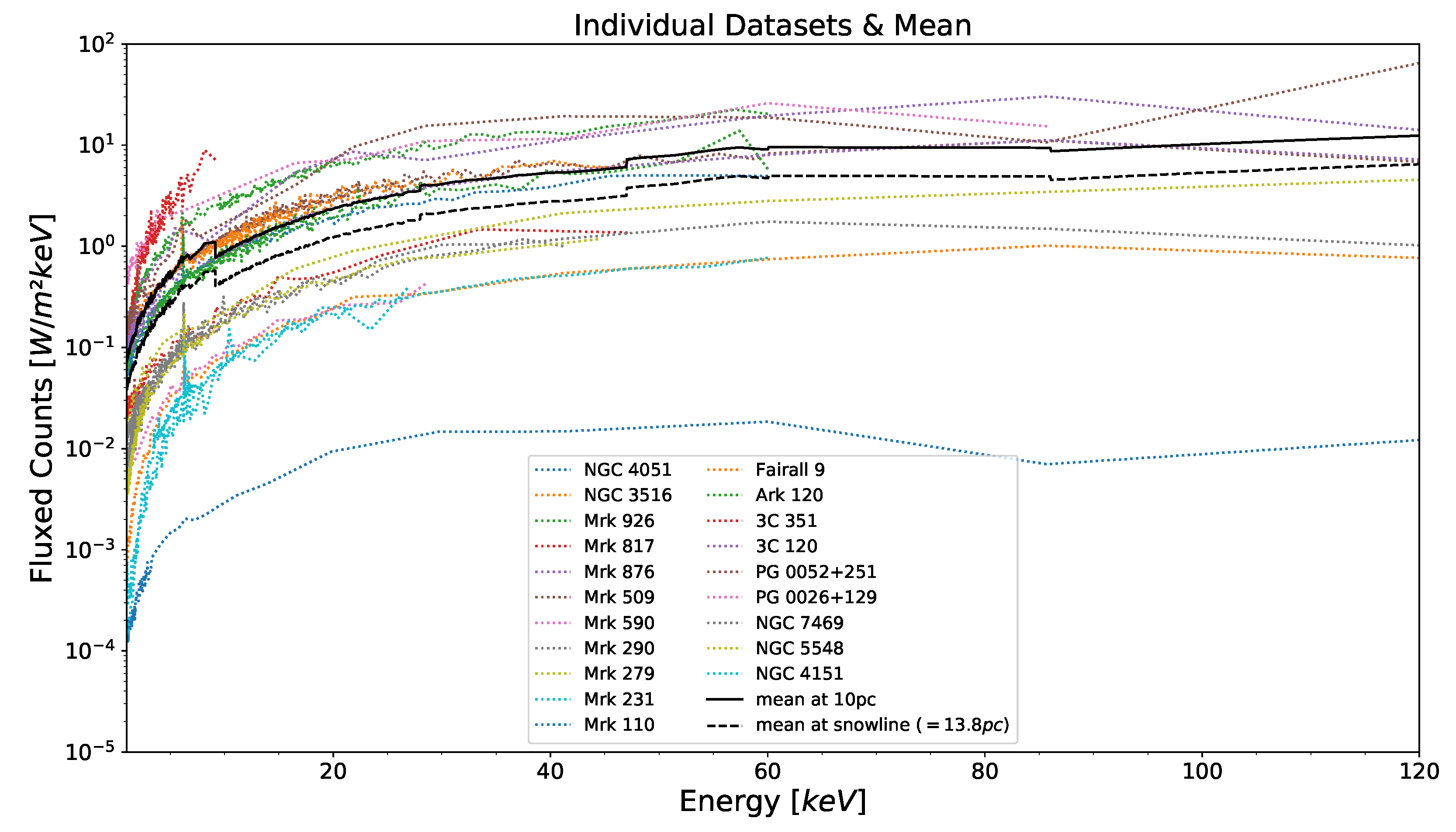
2.1. Obtaining a Mean Energy Spectrum
2.1.1. Adjusting Measurements for Distance and Angle
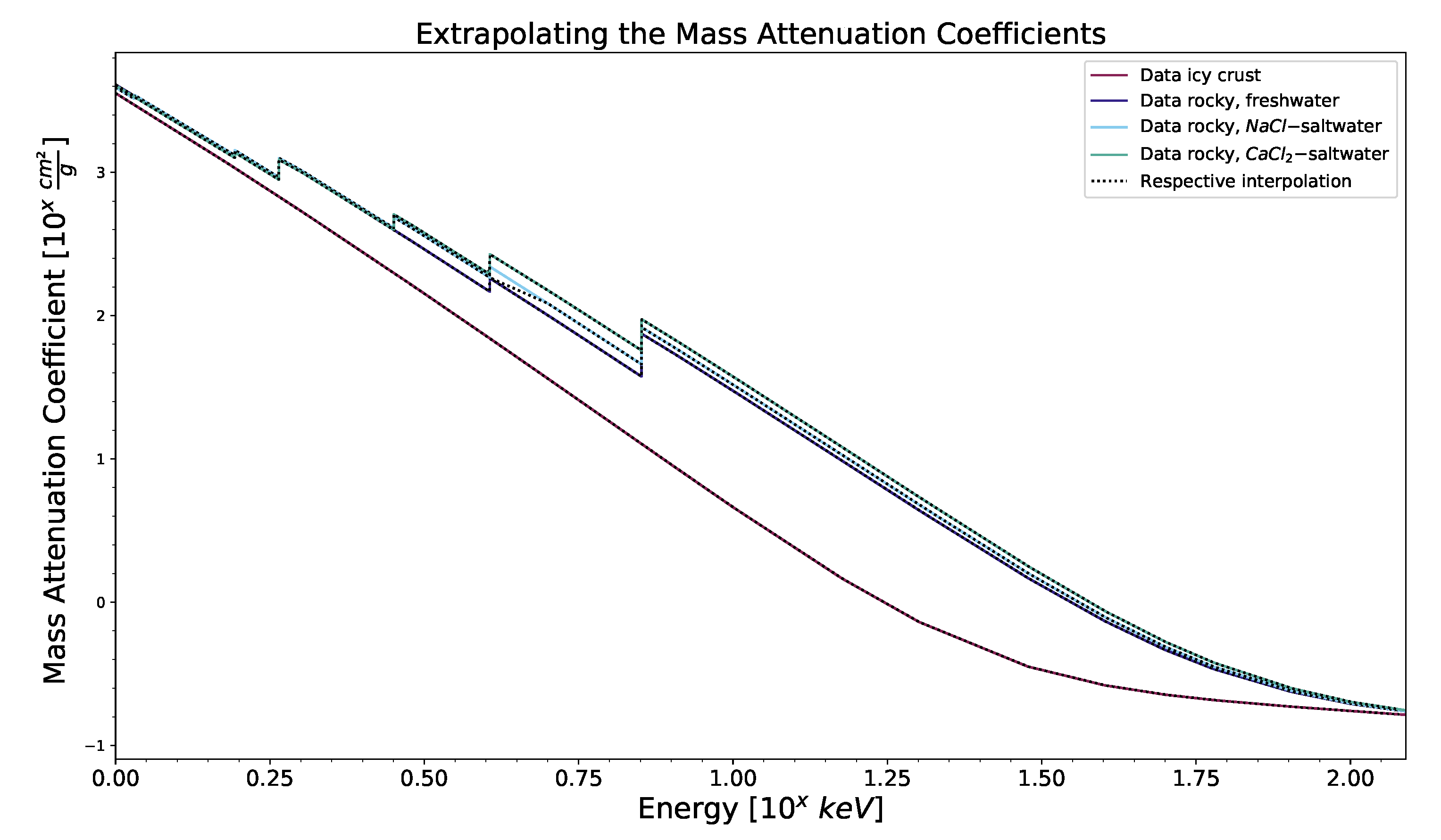
2.1.2. Interpolating and Averaging
2.2. Obtaining Surface Properties for Model Bodies
2.2.1. Proposing Surface Models
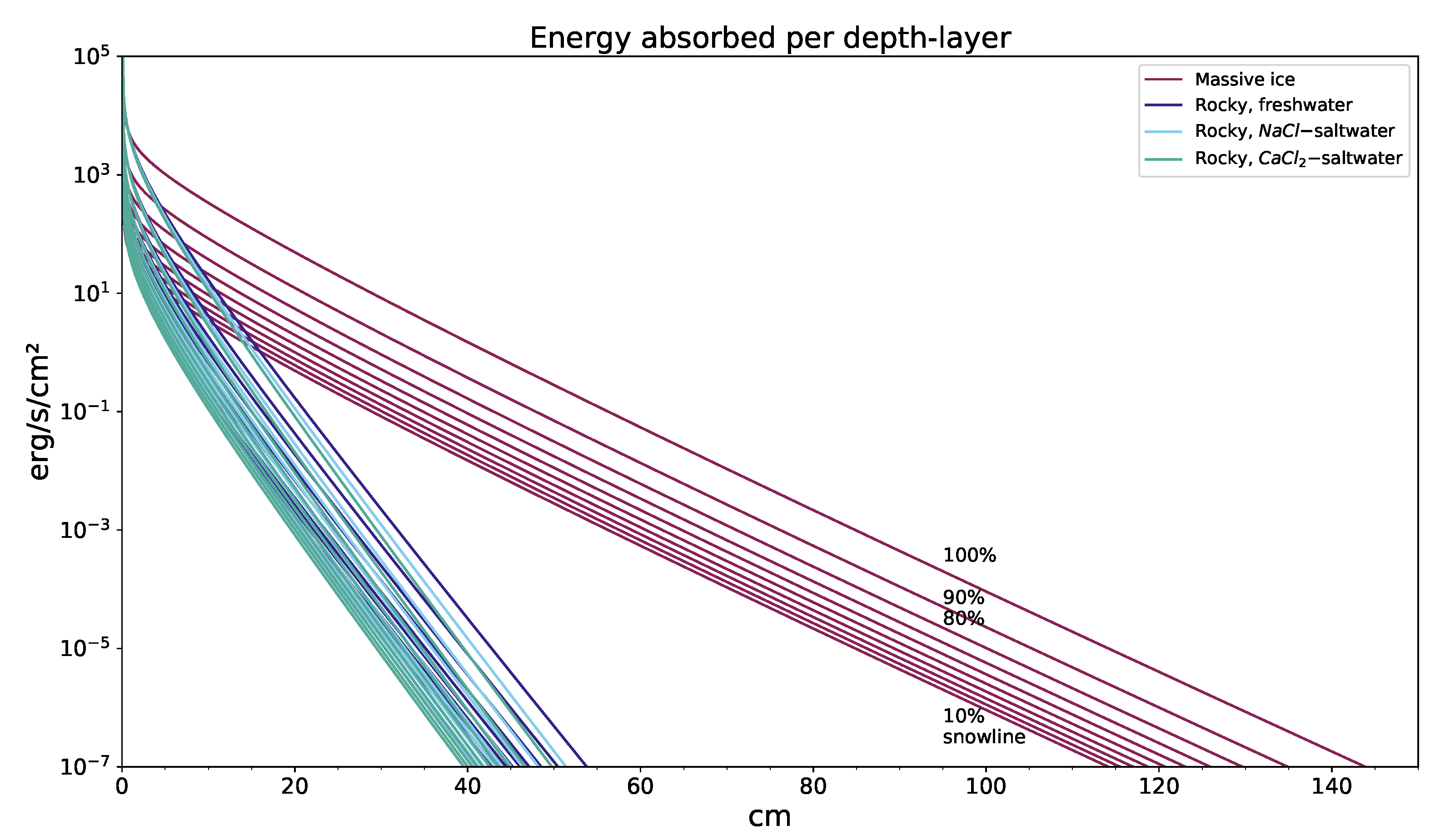
2.2.2. Calculating Attenuated Energy Using Lambert–Beer’s Law
2.2.3. Preparing Thermal Properties: Triple Point Depth
2.2.4. Vapor Pressure Curve
2.3. Simulating Thermal Profile within the Surface
2.3.1. Calculating Specific Heat Capacities Using Polynomial Equations
2.3.2. Setting Up a Solver for the 1-D Heat Equation
2.3.3. Forming a Frame for the Simulation with Continuous Input
2.4. Notes about IPython Multiprocessing for the Simulation
3. Results
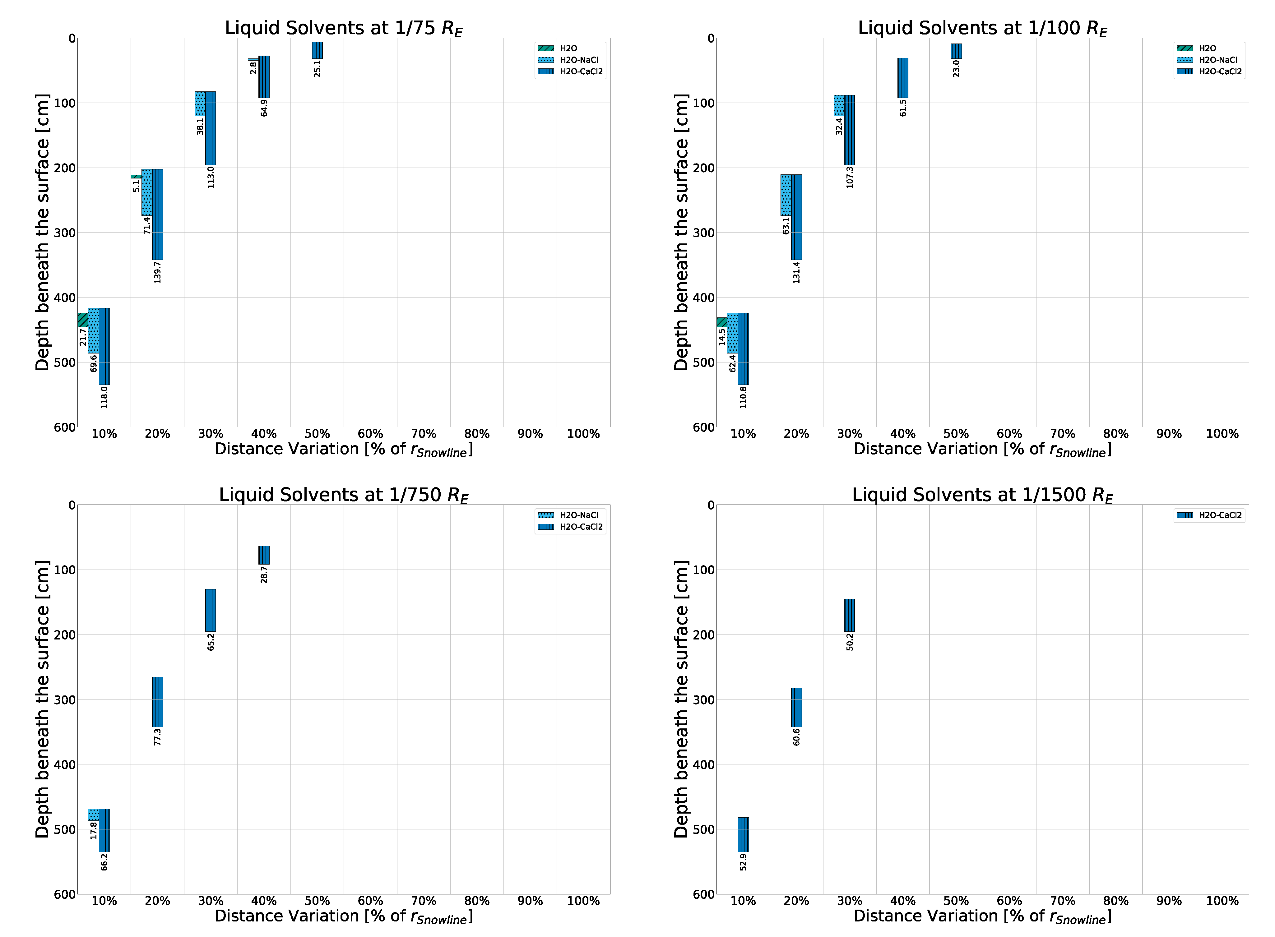
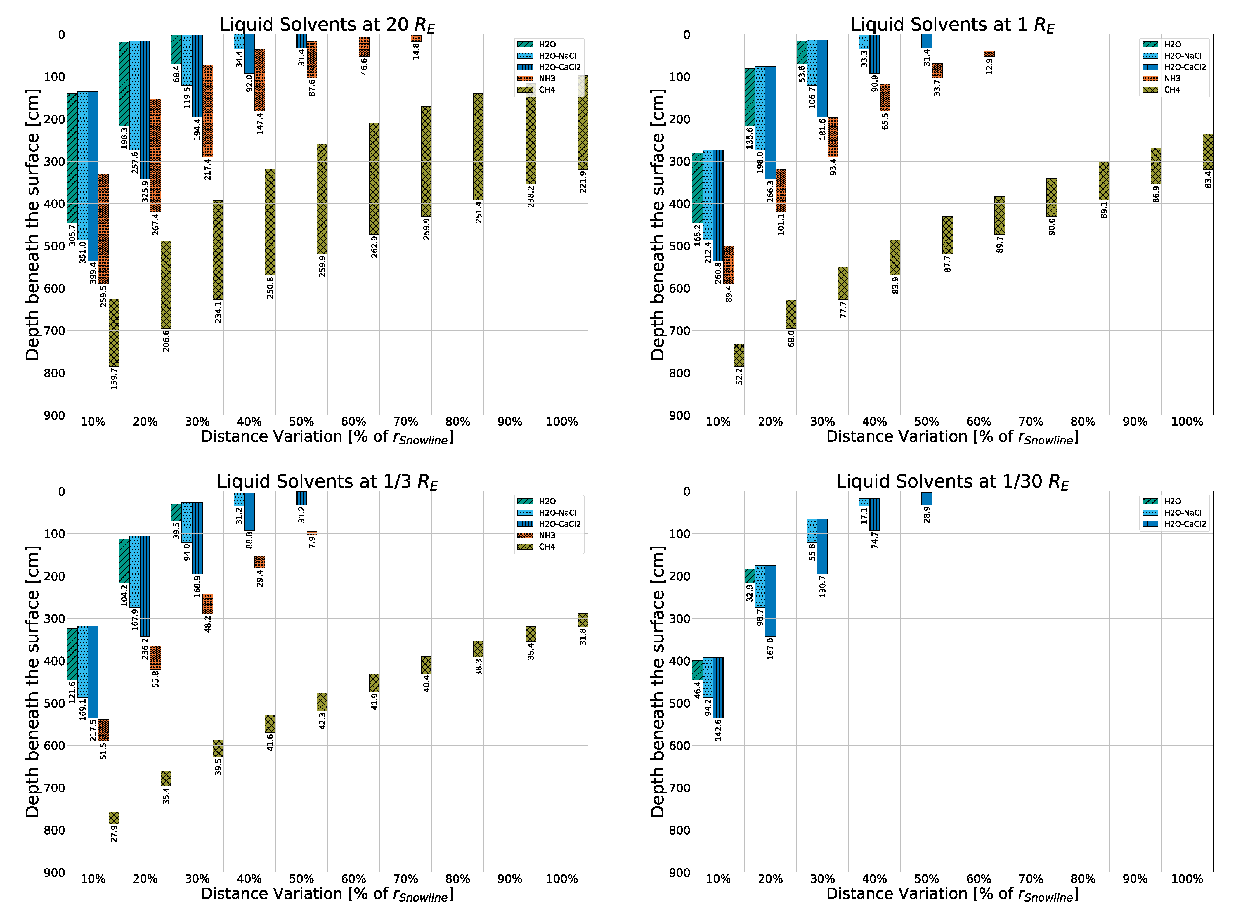
- It is possible for solvents to be liquid in bodies orbiting an AGN at a few parsecs of distance, fueled mainly by the X-ray emission of that AGN. This can happen in a somewhat wide variety of environments, with the AGN’s own energy output having much less of an impact compared to the density of a surface regolith (which greatly influences attenuation) or the size of the body itself (which greatly influences phase changes). The body’s inner density (beneath the regolith) plays a vital role as well, as seen in Appendix F.3. The influences are stronger for and .
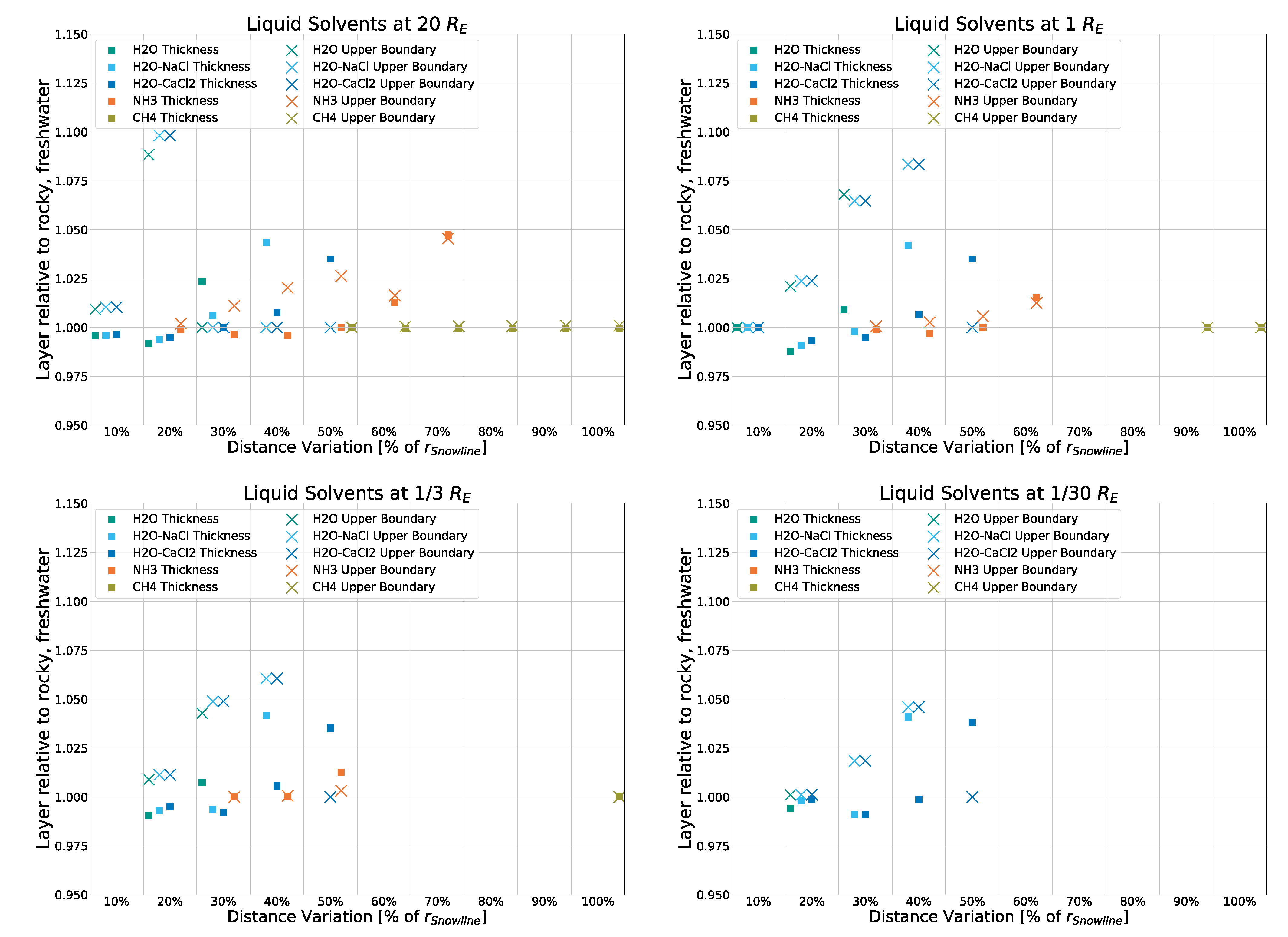
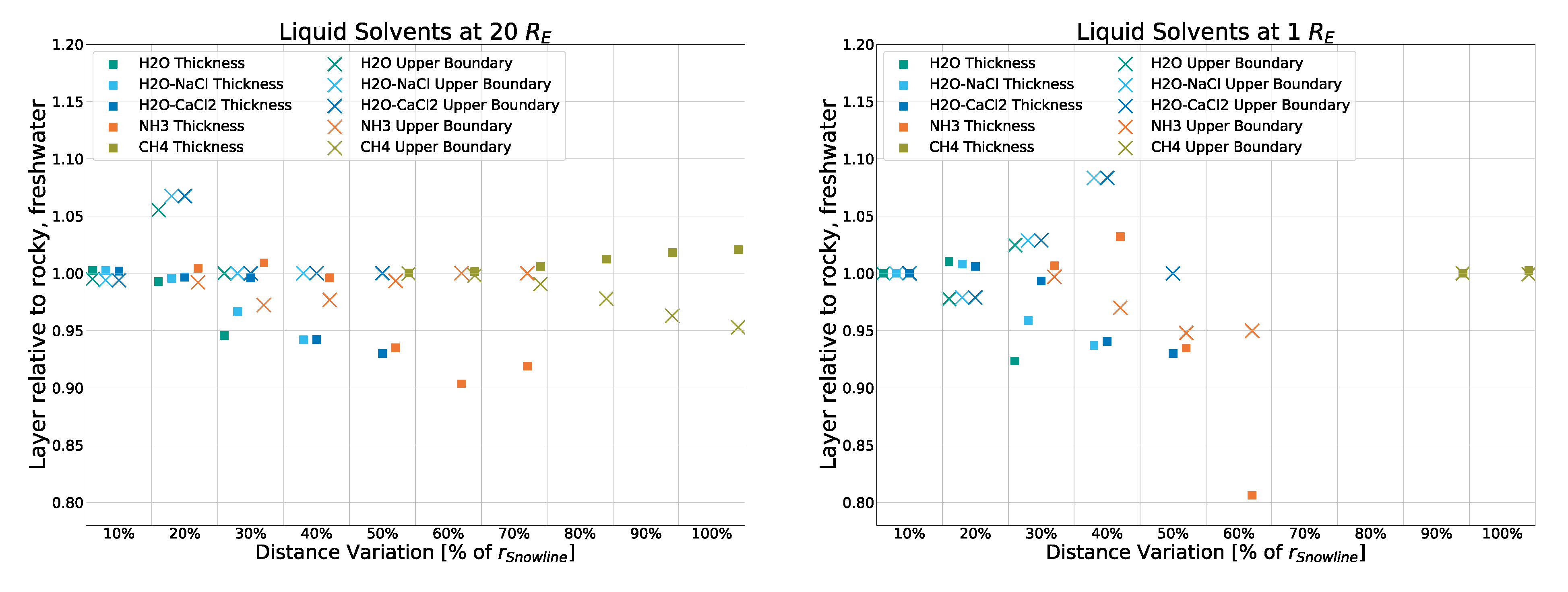
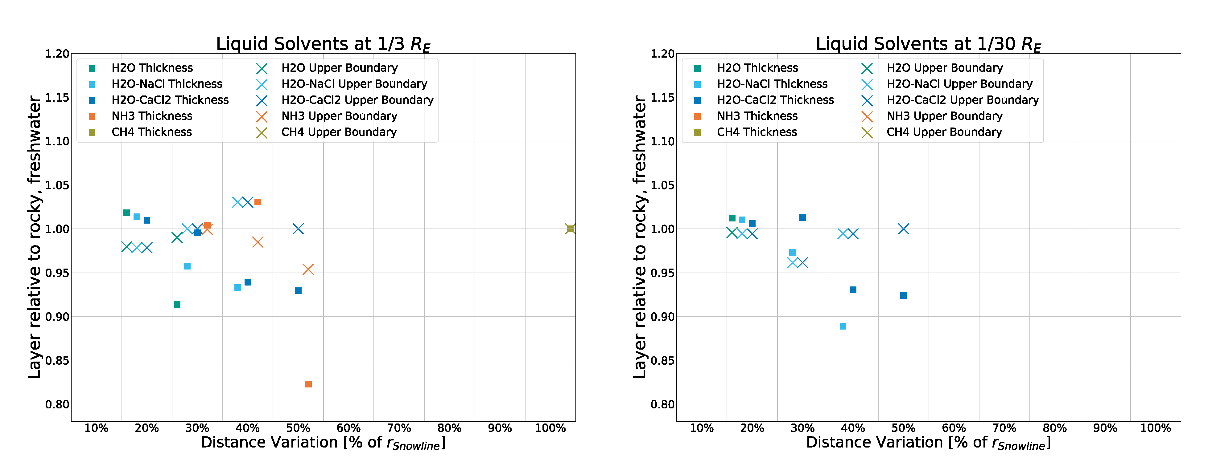
- The salt content of the optimal concentration can have a tremendously beneficial effect on the thermal properties of water in extreme environments (with this effect being more prominent for than ), and one can easily imagine that even away from the optimal concentration saltwater could beget liquidity on otherwise frozen worlds. However, in warmer environments, these effects can be slightly detrimental as compared to fresh water.
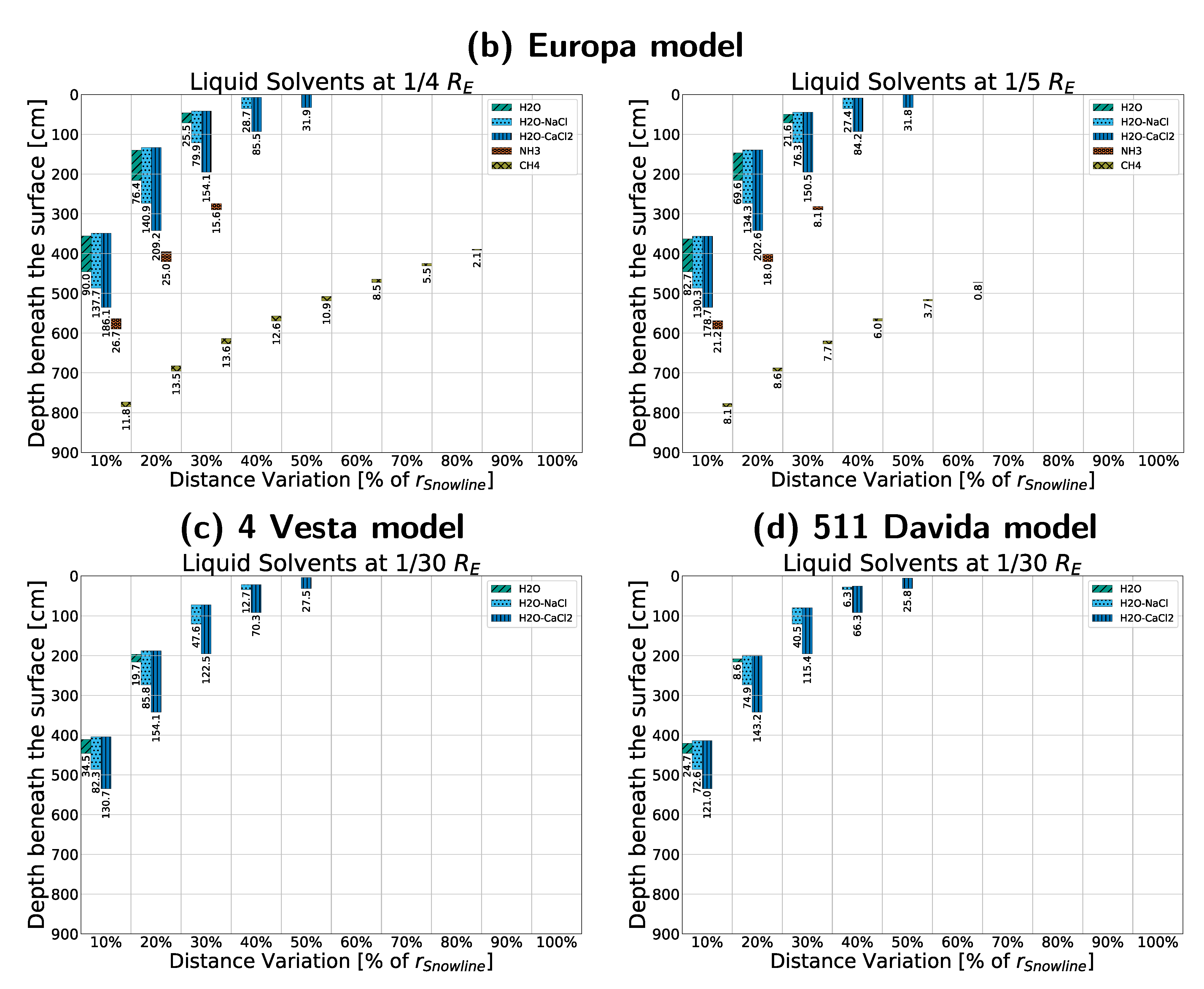
- Unsurprisingly, different solvents are constrained by different variables in this simulation, depending on the respective thermal properties. Water’s main constraint is temperature: Freezing points determine if and at what distance from the central source liquid layers can form, while boiling points mainly determine how deep within the crust this has to happen. On bodies too close to the central source, water close to the surface evaporates (the consequences of which would lead to stark alterations in the model itself that have not been considered here, as it would be beyond the scope of this paper), while water too far below would not be warm enough to melt. Methane and ammonia are constrained mainly by pressure, which allows these substances to be liquid even close to the snowline if the pressure is sufficient—so, if the body is large (and dense) enough.
4. Discussion
5. Conclusions
Author Contributions
Funding
Data Availability Statement
Acknowledgments
Conflicts of Interest
Abbreviations
| AGN | Active galactic nucleus |
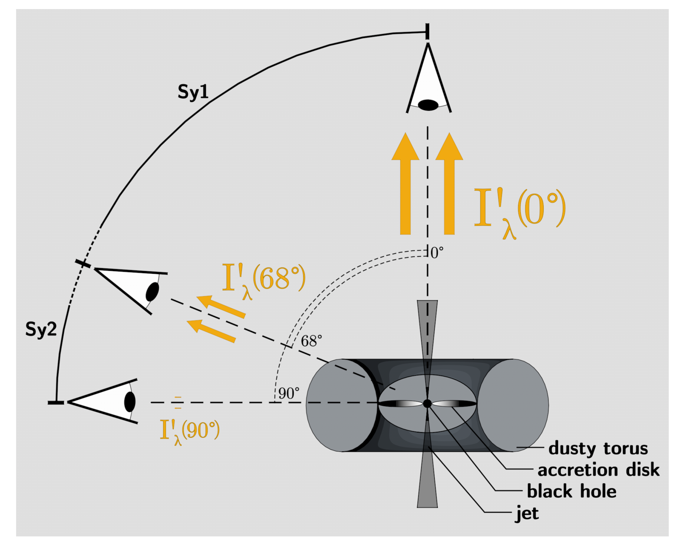
| Sy1 | Seyfert Type 1 |
| Sy2 | Seyfert Type 2 |
| CND | Circumnuclear disk |
| NIST | National Institute Of Standards Furthermore, Technology |
| CHERIC | Chemical Engineering and Materials Research Information Center |
| FTCS | Forward Time Centered Space |
| SIMBAD | Set of Identifications, Measurements and Bibliography for Astronomical Data |
Appendix A. Handling Distances and Viewing Angle of Investigated AGNs
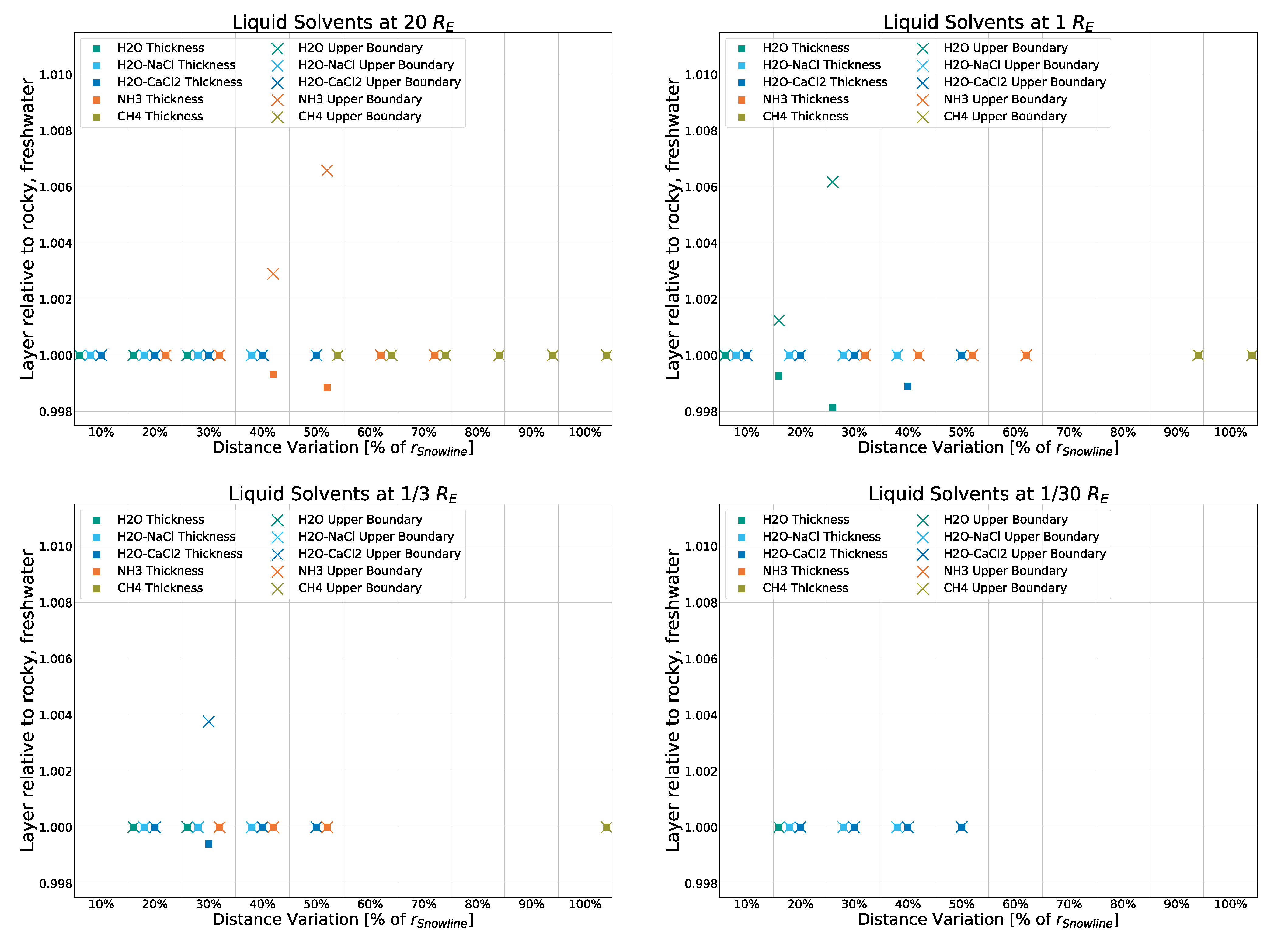
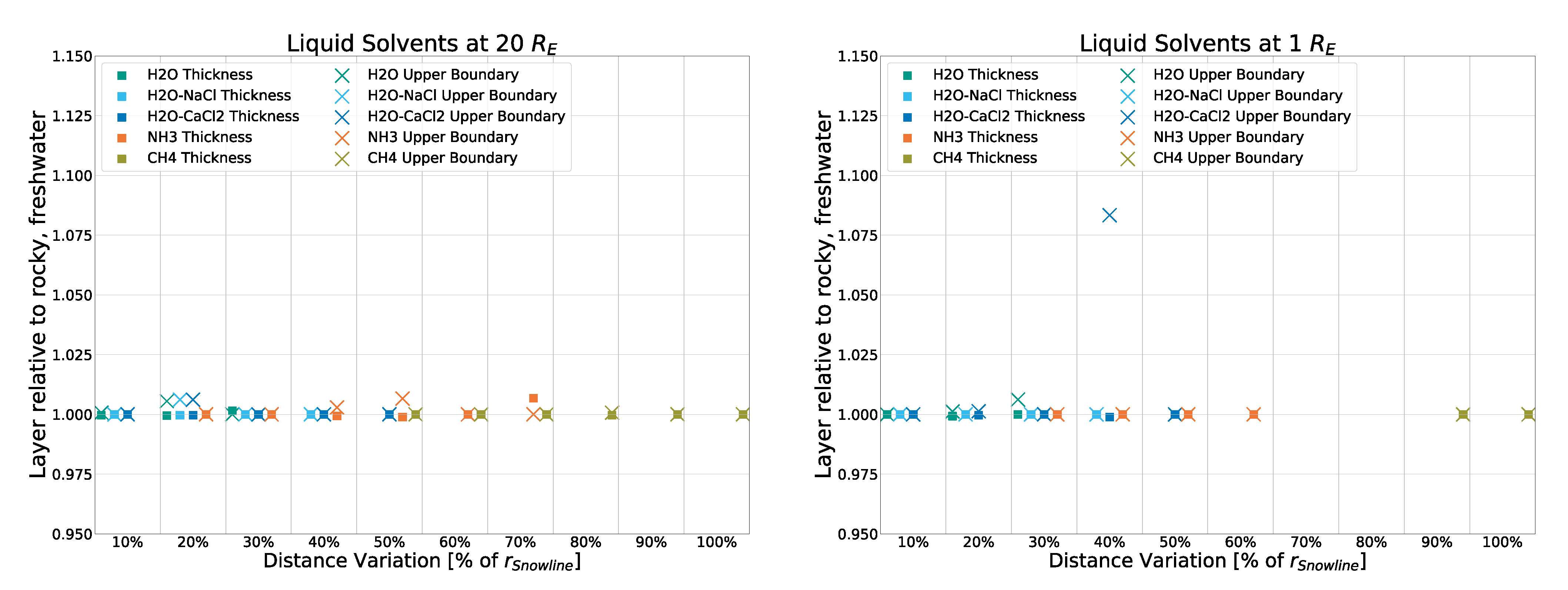
Appendix B. Exhaustive Model Simulations

Appendix C. Mass Attenuation Coefficient
Appendix D. About the Triple Point (Equivalent)
Appendix D.1. Triple Point (Equivalent) Properties

Appendix D.2. Derivation of Triple Point Depth
Appendix E. About Heat Conversion
| Substance | |||||
|---|---|---|---|---|---|
| 50 | 60 | 80 | 100 | 150 | |
| for | |||||
| water, liquid | 83.14 | 84.03 | 85.41 | 86.48 | 88.44 |
| glass | 83.64 | 84.77 | 86.36 | 87.49 | 89.44 |
| concrete | 83.12 | 84.33 | 85.99 | 87.17 | 89.17 |
| for | |||||
| water, liquid | 91.18 | 91.67 | 92.42 | 93.00 | 94.04 |
| glass | 91.45 | 92.07 | 92.93 | 93.54 | 94.57 |
| concrete | 91.17 | 91.83 | 92.73 | 93.36 | 94.43 |
| for | |||||
| water, liquid | 94.03 | 94.36 | 94.88 | 95.27 | 95.99 |
| glass | 94.22 | 94.64 | 95.23 | 95.64 | 96.35 |
| concrete | 94.02 | 94.48 | 95.09 | 95.53 | 96.25 |
Appendix F. Further Variabilities Investigated
Appendix F.3. Simulation on a Tidally Locked Body
Appendix F.4. Simulation with Individual Galaxies


Appendix F.5. Simulations of Small Moons and Asteroids

Appendix F.6. Determining the Minimum Valid Model Body Size
| 1 | |
| 2 | For the bulk of the simulations. Special calculations with systems as small as were carried out as well. |
| 3 | With data taken from the NIST WebBook [19]. |
| 4 | Only 90% of which will be used to generate the heat in this model however, with 10% being “reserved” for effects not inspected closer here such as secondary radiation and the modification of bonds of chemical compounds. This is discussed in detail in Appendix E. |
| 5 | Corresponding to the boiling point shift of these mixtures at these concentrations. |
| 6 | We do not account for lateral thermal decay as we are building a 1-D model, and horizontal thermal decay only occurs at the surface, which is controlled here using the equilibrium temperature. |
| 7 | Calculations were carried out in separate clusters, but plotting was carried out in the general IPython environment. This necessitates extra steps at this point that are laid out in more detail in Section 2.4. |
| 8 | Triple points are strictly speaking only defined for pure substances; we here use the critical point equivalent of a triple point as we are not interested in the exact phase behavior, merely the minimum pressure and temperature necessary for liquids to occur. |
References
- Stevenson, J.; Lunine, J.; Clancy, P. Membrane alternatives in worlds without oxygen: Creation of an azotosome. Sci. Adv. 2015, 1, e1400067. [Google Scholar] [CrossRef] [PubMed] [Green Version]
- Palmer, M.Y.; Cordiner, M.A.; Nixon, C.A.; Charnley, S.B.; Teanby, N.A.; Kisiel, Z.; Irwin, P.G.J.; Mumma, M.J. ALMA detection and astrobiological potential of vinyl cyanide on Titan. Sci. Adv. 2017, 3, e1700022. [Google Scholar] [CrossRef] [Green Version]
- Rampelotto, H.P. The search for life on other planets: Sulfur-based, silicon-based, ammonia-based life. J. Cosmol. 2010, 5, 818–827. [Google Scholar]
- Stofan, E.R.; Elachi, C.; Lunine, J.I.; Lorenz, R.D.; Stiles, B.; Mitchell, K.L.; Ostro, S.; Soderblom, L.; Wood, C.; Zebker, H.; et al. The lakes of Titan. Nature 2007, 445, 61–64. [Google Scholar] [CrossRef]
- Grasset, O.; Sotin, C.; Deschamps, F. On the internal structure and dynamics of Titan. Planet. Space Sci. 2000, 48, 617–636. [Google Scholar] [CrossRef]
- Wada, K.; Tsukamoto, Y.; Kokubo, E. Planet Formation around Supermassive Black Holes in the Active Galactic Nuclei. Astrophys. J. 2019, 886, 107. [Google Scholar] [CrossRef]
- Wada, K.; Tsukamoto, Y.; Kokubo, E. Formation of “Blanets” from Dust Grains around the Supermassive Black Holes in Galaxies. Astrophys. J. 2021, 909, 96. [Google Scholar] [CrossRef]
- Brown, M. An Atlas of Active Galactic Nuclei Spectral Energy Distributions (“AGNSEDATLAS”). Mon. Not. R. Astron. Soc. 2019, 489, 3351–3367. [Google Scholar] [CrossRef] [Green Version]
- Ginsburg, A.; Sipöcz, B.M.; Brasseur, C.E.; Cowperthwaite, P.S.; Craig, M.W.; Deil, C.; Guillochon, J.; Guzman, G.; Liedtke, S.; Lim, P.L.; et al. astroquery: An Astronomical Web-querying Package in Python. Astron. J. 2019, 157, 98. [Google Scholar] [CrossRef] [Green Version]
- Padovani, P. Active Galactic Nuclei at All Wavelengths and from All Angles. Front. Astron. Space Sci. 2017, 4, 35. [Google Scholar] [CrossRef] [Green Version]
- Fischer, T.C.; Crenshaw, D.M.; Kraemer, S.B.; Schmitt, H.R. Determining inclinations of active galactic nuclei via their narrow-line region kinematics. i. observational results. Astrophys. J. Suppl. Ser. 2013, 209, 1. [Google Scholar] [CrossRef]
- Antonucci, R. Unified Models for Active Galactic Nuclei and Quasars. Annu. Rev. Astron. Astrophys. 1993, 31, 473–521. [Google Scholar] [CrossRef]
- Zhang, S.N. A Single Intrinsic Luminosity Function for Both Type I and Type II Active Galactic Nuclei. Astrophys. J. 2004, 618, L79–L82. [Google Scholar] [CrossRef]
- Harris, C.R.; Millman, K.J.; van der Walt, S.J.; Gommers, R.; Virtanen, P.; Cournapeau, D.; Wieser, E.; Taylor, J.; Berg, S.; Smith, N.J.; et al. Array programming with NumPy. Nature 2020, 585, 357–362. [Google Scholar] [CrossRef]
- Virtanen, P.; Gommers, R.; Oliphant, T.E.; Haberland, M.; Reddy, T.; Cournapeau, D.; Burovski, E.; Peterson, P.; Weckesser, W.; Bright, J.; et al. SciPy 1.0: Fundamental Algorithms for Scientific Computing in Python. Nat. Methods 2020, 17, 261–272. [Google Scholar] [CrossRef] [PubMed] [Green Version]
- Alexander, L.; Snape, J.; Joy, K.; Downes, H.; Crawford, I. An analysis of Apollo lunar soil samples 12070,889, 12030,187, and 12070,891: Basaltic diversity at the Apollo 12 landing site and implications for classification of small-sized lunar samples. Meteorit. Planet. Sci. 2016, 51, 1654–1677. [Google Scholar] [CrossRef]
- Kreidberg, L.; Koll, D.D.B.; Morley, C.; Hu, R.; Schaefer, L.; Deming, D.; Stevenson, K.B.; Dittmann, J.; Vanderburg, A.; Berardo, D.; et al. Absence of a thick atmosphere on the terrestrial exoplanet LHS 3844b. Nature 2019, 573, 87–90. [Google Scholar] [CrossRef] [PubMed] [Green Version]
- Harada, N.; Riquelme, D.; Viti, S.; Jiménez-Serra, I.; Requena-Torres, M.A.; Menten, K.M.; Martín, S.; Aladro, R.; Martin-Pintado, J.; Hochgürtel, S. Chemical features in the circumnuclear disk of the Galactic center. Astron. Astrophys. 2015, 584, A102. [Google Scholar] [CrossRef] [Green Version]
- Thermodynamics Research Center; NIST Boulder Lab.; Muzny, C. Thermodynamics Source Database. In NIST Chemistry WebBook, NIST Standard Reference Database 69; Linstrom, P.J., Mallard, W.G., Eds.; National Institute of Standards and Technology: Gaithersburg, MD, USA, 1997. [Google Scholar] [CrossRef]
- XCOM. NIST XCOM Selection. 2010. Available online: https://physics.nist.gov/PhysRefData/Xcom/html/xcom1.html (accessed on 25 October 2021).
- CHERIC. CHERIC Pure Component Properties. 2011. Available online: https://www.cheric.org/research/kdb/hcprop/cmpsrch.php (accessed on 23 October 2021).
- Landau, L.D.; Lifshitz, E.M. Statistical Physics Part 1; Pergamon Press: Oxford, UK, 1980; pp. 193–196. [Google Scholar]
- Overstreet, R.; Giauque, W.F. Ammonia. The Heat Capacity and Vapor Pressure of Solid and Liquid. Heat of Vaporization. The Entropy Values from Thermal and Spectroscopic Data. J. Am. Chem. Soc. 1937, 59, 254–259. [Google Scholar] [CrossRef]
- Yakub, L.; Bodiul, O. Low-temperature equation of state of solid methane. Refrig. Eng. Technol. 2016, 52, 80–85. [Google Scholar] [CrossRef]
- Shulman, L.M. The heat capacity of water ice in interstellar or interplanetary conditions. Astron. Astrophys. 2004, 416, 187–190. [Google Scholar] [CrossRef]
- Riflet, G. 1D Heat Equation and a Finite-Difference Solver. 2010. Available online: https://fenix.tecnico.ulisboa.pt/downloadFile/3779573658038/HeatEquation.pdf (accessed on 3 January 2020).
- Perez, F.; Granger, B.E. IPython: A System for Interactive Scientific Computing. Comput. Sci. Eng. 2007, 9, 21–29. [Google Scholar] [CrossRef]
- Hunter, J.D. Matplotlib: A 2D Graphics Environment. Comput. Sci. Eng. 2007, 9, 90–95. [Google Scholar] [CrossRef]
- Nelson, R.M.; Boryta, M.D.; Hapke, B.W.; Shkuratov, Y.; Vandervoort, K.; Vides, C.L. Understanding Europa’s Surface Texture from Remote Sensing Photopolarimetry. In Proceedings of the AGU Fall Meeting Abstracts, San Francisco, CA, USA, 12–16 December 2016. abstract id. P11C–1870. [Google Scholar]
- Mitri, G.; Showman, A.; Lunine, J.; Lopes, R. Cryovolcanism on Titan. In Proceedings of the AGU Fall Meeting Abstracts, San Francisco, CA, USA, 15–19 December 2008. [Google Scholar]
- Fritsen, C.H.; Coale, S.L.; Neenan, D.R.; Gibson, A.H.; Garrison, D.L. Biomass, production and microhabitat characteristics near the freeboard of ice floes in the Ross Sea, Antarctica, during the austral summer. Ann. Glaciol. 2001, 33, 280–286. [Google Scholar] [CrossRef] [Green Version]
- Meckenstock, R.U.; von Netzer, F.; Stumpp, C.; Lueders, T.; Himmelberg, A.M.; Hertkorn, N.; Schmitt-Kopplin, P.; Harir, M.; Hosein, R.; Haque, S.; et al. Water droplets in oil are microhabitats for microbial life. Science 2014, 345, 673–676. [Google Scholar] [CrossRef]
- da Silva, T.H.; Silva, D.A.S.; Thomazini, A.; Schaefer, C.E.G.R.; Rosa, L.H. Antarctic Permafrost: An Unexplored Fungal Microhabitat at the Edge of Life. In Fungi of Antarctica: Diversity, Ecology and Biotechnological Applications; Rosa, L.H., Ed.; Springer International Publishing: Cham, Switzerland, 2019; Volume 345, pp. 147–164. [Google Scholar] [CrossRef]
- Kennedy, A. Antarctic Permafrost: An Unexplored Fungal Microhabitat at the Edge of Life. Antarct. Sci. 1999, 11, 27–37. [Google Scholar] [CrossRef]
- Glass, T.W.; Breed, G.A.; Iwahana, G.; Kynoch, M.C.; Robards, M.D.; Williams, C.T.; Kielland, K. Permafrost ice caves: An unrecognized microhabitat for Arctic wildlife. Ecology 2021, 102, e03276. [Google Scholar] [CrossRef]
- Altair, T.; de Avellar, M.G.B.; Rodrigues, F.; Galante, D. Microbial habitability of Europa sustained by radioactive sources. Sci. Rep. 2018, 8, 260. [Google Scholar] [CrossRef] [Green Version]
- Braun, S.; Morono, Y.; Littmann, S.; Kuypers, M.; Aslan, H.; Dong, M.; Jørgensen, B.B.; Lomstein, B.A. Size and Carbon Content of Sub-seafloor Microbial Cells at Landsort Deep, Baltic Sea. Front. Microbiol. 2016, 7, 1375. [Google Scholar] [CrossRef]
- Khetan, N.; Izzo, L.; Branchesi, M.; Wojtak, R.; Cantiello, M.; Murugeshan, C.; Agnello, A.; Cappellaro, E.; Della Valle, M.; Gall, C.; et al. A new measurement of the Hubble constant using Type Ia supernovae calibrated with surface brightness fluctuations. Astron. Astrophys. 2021, 647, A72. [Google Scholar] [CrossRef]
- Bodnar, R.J. PTX Phase Equilibria in the H2O-CO2-Salt System at Mars Near-Surface Conditions. In Proceedings of the Lunar and Planetary Science Conference, Houston, TX, USA, 12–16 March 2001; p. 1689. [Google Scholar]
- Ketcham, S.A.; Minsk, L.D.; Blackburn, R.R.; Fleege, E.J. Manual of Practice for an Effective Anti-Icing Program; Turner-Fairbank Highway Research Center: McLean, VA, USA, 1996; Publication Number: FHWA-RD-95-202. [Google Scholar]
- Williams, D. Earth Fact Sheet. 2020. Available online: https://nssdc.gsfc.nasa.gov/planetary/factsheet/earthfact.html (accessed on 12 April 2021).
- Hubbell, J.H.; Seltzer, S.M. Tables of X-Ray Mass Attenuation Coefficients and Mass Energy-Absorption Coefficients (Version 1.4); National Institute of Standards and Technology: Gaithersburg, MD, USA, 2004. Available online: http://physics.nist.gov/xaamdi (accessed on 5 January 2020). [CrossRef]
- Showman, A.P.; Malhotra, R. The Galilean Satellites. Science 1999, 286, 77–84. [Google Scholar] [CrossRef] [PubMed] [Green Version]
- Carry, B. Density of asteroids. Planet. Space Sci. 2012, 73, 98–118. [Google Scholar] [CrossRef] [Green Version]
- Hui, M.T.; Jewitt, D.; Yu, L.L.; Mutchler, M.J. Hubble Space Telescope Detection of the Nucleus of Comet C/2014 UN271 (Bernardinelli-Bernstein). Astrophys. J. Lett. 2022, 929, L12. [Google Scholar] [CrossRef]
- Lellouch, E.; Moreno, R.; Bockelée-Morvan, D.; Biver, N.; Santos-Sanz, P. Size and albedo of the largest detected Oort-cloud object: Comet C/2014 UN271 (Bernardinelli-Bernstein). Astron. Astrophys. 2022, 659, L1. [Google Scholar] [CrossRef]

| Formula | Abundances | |||
|---|---|---|---|---|
| Icy Composition | Rocky Composition | |||
| Ice | Fresh a | b | c | |
| 0.762 | 0.381 | 0.293 | 0.263 | |
| 0.17 | 0.085 | 0.085 | 0.085 | |
| 0.068 | 0.034 | 0.034 | 0.034 | |
| 0.25 | 0.25 | 0.25 | ||
| 0.135 | 0.135 | 0.135 | ||
| 0.06 | 0.06 | 0.06 | ||
| 0.055 | 0.055 | 0.055 | ||
| 0.088 | ||||
| 0.118 | ||||
| Surface Model | Density |
|---|---|
| Rocky, freshwater | |
| Rocky, -saltwater | |
| Rocky, -saltwater | |
| Icy |
| Formula | Coefficients a | ||
|---|---|---|---|
| A | B | C | |
Publisher’s Note: MDPI stays neutral with regard to jurisdictional claims in published maps and institutional affiliations. |
© 2022 by the authors. Licensee MDPI, Basel, Switzerland. This article is an open access article distributed under the terms and conditions of the Creative Commons Attribution (CC BY) license (https://creativecommons.org/licenses/by/4.0/).
Share and Cite
Rodener, D.; Schäfer, M.; Hausmann, M.; Hildenbrand, G. Assessing the Potential for Liquid Solvents from X-ray Sources: Considerations on Bodies Orbiting Active Galactic Nuclei. Galaxies 2022, 10, 101. https://doi.org/10.3390/galaxies10050101
Rodener D, Schäfer M, Hausmann M, Hildenbrand G. Assessing the Potential for Liquid Solvents from X-ray Sources: Considerations on Bodies Orbiting Active Galactic Nuclei. Galaxies. 2022; 10(5):101. https://doi.org/10.3390/galaxies10050101
Chicago/Turabian StyleRodener, Daniel, Myriam Schäfer, Michael Hausmann, and Georg Hildenbrand. 2022. "Assessing the Potential for Liquid Solvents from X-ray Sources: Considerations on Bodies Orbiting Active Galactic Nuclei" Galaxies 10, no. 5: 101. https://doi.org/10.3390/galaxies10050101