
Comparison of Early Contrast Enhancement Models in Ultrafast Dynamic Contrast-Enhanced Magnetic Resonance Imaging of Prostate Cancer
 , , ,
, , ,
Abstract
:1. Introduction
2. Materials and Methods
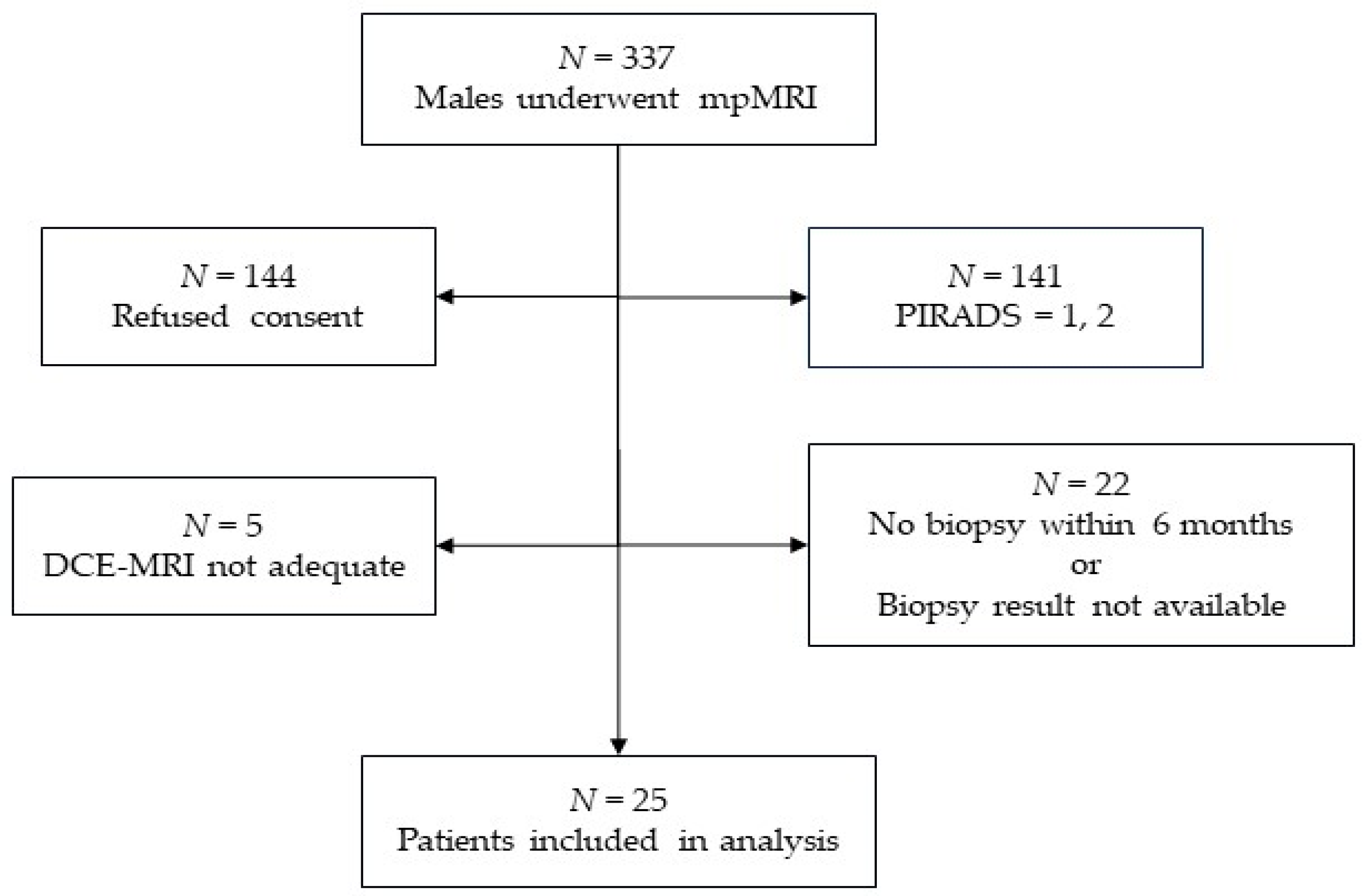
2.1. Patients
- Adult males between 40 and 85 years of age;
- With one or more lesions having a PI-RADS category of 3, 4, or 5;
- Prostate biopsy targeted to the reported lesion(s) within 6 months of the mpMRI examination.
- Prior local or systemic treatment for prostate cancer;
- Examinations performed without injection of contrast agent;
- Contraindications to MRI.
2.2. DCE-MRI Acquisition
2.3. DCE-MRI Processing
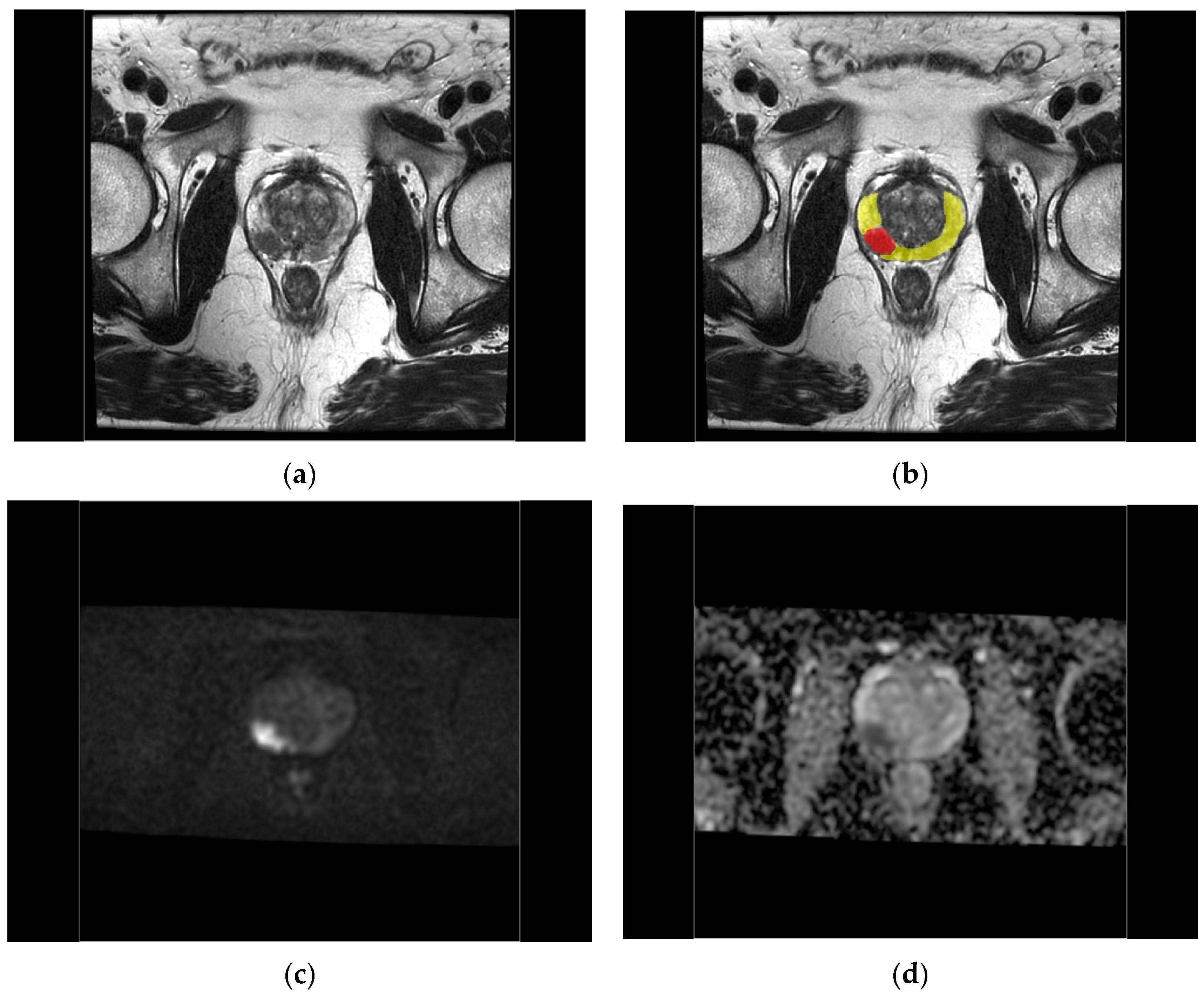
2.4. Region of Interest Definition
2.5. Radiological and Pathological Evaluation
2.6. Statistical Analysis
3. Results
4. Discussion
5. Conclusions
Supplementary Materials
Author Contributions
Funding
Institutional Review Board Statement
Informed Consent Statement
Data Availability Statement
Conflicts of Interest
References
- Turkbey, B.; Rosenkrantz, A.B.; Haider, M.A.; Padhani, A.R.; Villeirs, G.; Macura, K.J.; Tempany, C.M.; Choyke, P.L.; Cornud, F.; Margolis, D.J.; et al. Prostate Imaging Reporting and Data System Version 2.1: 2019 Update of Prostate Imaging Reporting and Data System Version 2. Eur. Urol. 2019, 76, 340–351. [Google Scholar] [CrossRef]
- Chatterjee, A.; He, D.; Fan, X.; Wang, S.; Szasz, T.; Yousuf, A.; Pineda, F.; Antic, T.; Mathew, M.; Karczmar, G.S.; et al. Performance of Ultrafast DCE-MRI for Diagnosis of Prostate Cancer. Acad. Radiol. 2018, 25, 349–358. [Google Scholar] [CrossRef] [PubMed]
- Rosenkrantz, A.B.; Geppert, C.; Grimm, R.; Block, T.K.; Glielmi, C.; Feng, L.; Otazo, R.; Ream, J.M.; Romolo, M.M.; Taneja, S.S.; et al. Dynamic contrast-enhanced MRI of the prostate with high spatiotemporal resolution using compressed sensing, parallel imaging, and continuous golden-angle radial sampling: Preliminary experience. J. Magn. Reson. Imaging 2015, 41, 1365–1373. [Google Scholar] [CrossRef] [PubMed]
- Sourbron, S.P.; Buckley, D.L. On the scope and interpretation of the Tofts models for DCE-MRI. Magn. Reson. Med. 2011, 66, 735–745. [Google Scholar] [CrossRef]
- Tofts, P.S. Modeling tracer kinetics in dynamic Gd-DTPA MR imaging. J. Magn. Reson. Imaging 1997, 7, 91–101. [Google Scholar] [CrossRef] [PubMed]
- Tofts, P.S.; Brix, G.; Buckley, D.L.; Evelhoch, J.L.; Henderson, E.; Knopp, M.V.; Larsson, H.B.; Lee, T.Y.; Mayr, N.A.; Parker, G.J.; et al. Estimating kinetic parameters from dynamic contrast-enhanced T(1)-weighted MRI of a diffusable tracer: Standardized quantities and symbols. J. Magn. Reson. Imaging 1999, 10, 223–232. [Google Scholar] [CrossRef]
- Sourbron, S.P.; Buckley, D.L. Tracer kinetic modelling in MRI: Estimating perfusion and capillary permeability. Phys. Med. Biol. 2012, 57, R1–R33. [Google Scholar] [CrossRef]
- Berks, M.; Little, R.A.; Watson, Y.; Cheung, S.; Datta, A.; O’Connor, J.P.B.; Scaramuzza, D.; Parker, G.J.M. A model selection framework to quantify microvascular liver function in gadoxetate-enhanced MRI: Application to healthy liver, diseased tissue, and hepatocellular carcinoma. Magn. Reson. Med. 2021, 86, 1829–1844. [Google Scholar] [CrossRef] [PubMed]
- Kallehauge, J.F.; Sourbron, S.; Irving, B.; Tanderup, K.; Schnabel, J.A.; Chappell, M.A. Comparison of linear and nonlinear implementation of the compartmental tissue uptake model for dynamic contrast-enhanced MRI. Magn. Reson. Med. 2017, 77, 2414–2423. [Google Scholar] [CrossRef]
- Sourbron, S.; Ingrisch, M.; Siefert, A.; Reiser, M.; Herrmann, K. Quantification of cerebral blood flow, cerebral blood volume, and blood-brain-barrier leakage with DCE-MRI. Magn. Reson. Med. 2009, 62, 205–217. [Google Scholar] [CrossRef]
- Tofts, P.; Parker, G.J.M. DCE-MRI: Acquisition and analysis techniques. In Clinical Perfusion MRI: Techniques and Applications; Barker, P., Golay, X., Zaharchuk, G., Eds.; Cambridge University Press: Cambridge, UK, 2013; pp. 58–74. ISBN 9781139004053. [Google Scholar] [CrossRef]
- Ingrisch, M.; Sourbron, S. Tracer-kinetic modeling of dynamic contrast-enhanced MRI and CT: A primer. J. Pharmacokinet. Pharmacodyn. 2013, 40, 281–300. [Google Scholar] [CrossRef] [PubMed]
- Fan, X.; Medved, M.; River, J.N.; Zamora, M.; Corot, C.; Robert, P.; Bourrinet, P.; Lipton, M.; Culp, R.M.; Karczmar, G.S.; et al. New model for analysis of dynamic contrast-enhanced MRI data distinguishes metastatic from nonmetastatic transplanted rodent prostate tumors. Magn. Reson. Med. 2004, 51, 487–494. [Google Scholar] [CrossRef] [PubMed]
- Fan, X.; Medved, M.; Karczmar, G.S.; Yang, C.; Foxley, S.; Arkani, S.; Recant, W.; Zamora, M.A.; Abe, H.; Newstead, G.M. Diagnosis of suspicious breast lesions using an empirical mathematical model for dynamic contrast-enhanced MRI. Magn. Reson. Imaging 2007, 25, 593–603. [Google Scholar] [CrossRef] [PubMed]
- Saranathan, M.; Rettmann, D.W.; Hargreaves, B.A.; Clarke, S.E.; Vasanawala, S.S. DIfferential Subsampling with Cartesian Ordering (DISCO): A high spatio-temporal resolution Dixon imaging sequence for multiphasic contrast enhanced abdominal imaging. J. Magn. Reson. Imaging 2012, 35, 1484–1492. [Google Scholar] [CrossRef]
- Workie, D.W.; Dardzinski, B.J.; Graham, T.B.; Laor, T.; Bommer, W.A.; O’Brien, K.J. Quantification of dynamic contrast-enhanced MR imaging of the knee in children with juvenile rheumatoid arthritis based on pharmacokinetic modeling. Magn. Reson. Imaging 2004, 22, 1201–1210. [Google Scholar] [CrossRef] [PubMed]
- Berks, M.; Parker, G.J.M.; Little, R.; Cheung, S. Madym: A C++ toolkit for quantitative DCE-MRI analysis. J. Open Source Softw. 2021, 6, 3523. [Google Scholar] [CrossRef]
- Epstein, J.I.; Egevad, L.; Amin, M.B.; Delahunt, B.; Srigley, J.R.; Humphrey, P.A.; Grading Committee. The 2014 International Society of Urological Pathology (ISUP) Consensus Conference on Gleason Grading of Prostatic Carcinoma: Definition of Grading Patterns and Proposal for a New Grading System. Am. J. Surg. Pathol. 2016, 40, 244–252. [Google Scholar] [CrossRef] [PubMed]
- Bastian-Jordan, M. Magnetic resonance imaging of the prostate and targeted biopsy, Comparison of PIRADS and Gleason grading. J. Med. Imaging Radiat. Oncol. 2018, 62, 183–187. [Google Scholar] [CrossRef] [PubMed]
- Kızılay, F.; Çelik, S.; Sözen, S.; Özveren, B.; Eskiçorapçı, S.; Özgen, M.; Özen, H.; Akdoğan, B.; Aslan, G.; Narter, F.; et al. Correlation of Prostate-Imaging Reporting and Data Scoring System scoring on multiparametric prostate magnetic resonance imaging with histopathological factors in radical prostatectomy material in Turkish prostate cancer patients: A multicenter study of the Urooncology Association. Prostate Int. 2020, 8, 10–15. [Google Scholar] [CrossRef]
- Verma, S.; Turkbey, B.; Muradyan, N.; Rajesh, A.; Cornud, F.; Haider, M.A.; Choyke, P.L.; Harisinghani, M. Overview of dynamic contrast-enhanced MRI in prostate cancer diagnosis and management. Am. J. Roentgenol. 2012, 198, 1277–1288. [Google Scholar] [CrossRef]
- Wei, C.; Jin, B.; Szewczyk-Bieda, M.; Gandy, S.; Lang, S.; Zhang, Y.; Huang, Z.; Nabi, G. Quantitative parameters in dynamic contrast-enhanced magnetic resonance imaging for the detection and characterization of prostate cancer. Oncotarget 2018, 9, 15997–16007. [Google Scholar] [CrossRef] [PubMed]
- Hötker, A.M.; Mazaheri, Y.; Aras, Ö.; Zheng, J.; Moskowitz, C.S.; Gondo, T.; Matsumoto, K.; Hricak, H.; Akin, O. Assessment of Prostate Cancer Aggressiveness by Use of the Combination of Quantitative DWI and Dynamic Contrast-Enhanced MRI. Am. J. Roentgenol. 2016, 206, 756–763. [Google Scholar] [CrossRef]
- Meyer, H.-J.; Wienke, A.; Surov, A. Can dynamic contrast enhanced MRI predict Gleason score in prostate cancer? a systematic review and meta analysis. Urol. Oncol. 2021, 39, e17–e25. [Google Scholar] [CrossRef]
- He, D.; Fan, X.; Chatterjee, A.; Wang, S.; Medved, M.; Pineda, F.D.; Yousuf, A.; Antic, T.; Oto, A.; Karczmar, G.S. A compact solution for estimation of physiological parameters from ultrafast prostate dynamic contrast enhanced MRI. Phys. Med. Biol. 2019, 64, 155012. [Google Scholar] [CrossRef]
- Mustafi, D.; Gleber, S.C.; Ward, J.; Dougherty, U.; Zamora, M.; Markiewicz, E.; Binder, D.C.; Antic, T.; Vogt, S.; Karczmar, G.S.; et al. IV Administered Gadodiamide Enters the Lumen of the Prostatic Glands: X-Ray Fluorescence Microscopy Examination of a Mouse Model. Am. J. Roentgenol. 2015, 205, W313–W319. [Google Scholar] [CrossRef] [PubMed]
- Noworolski, S.M.; Vigneron, D.B.; Chen, A.P.; Kurhanewicz, J. Dynamic contrast-enhanced MRI and MR diffusion imaging to distinguish between glandular and stromal prostatic tissues. Magn. Reson. Imaging. 2008, 26, 1071–1080. [Google Scholar] [CrossRef] [PubMed]
- Guljaš, S.; Dupan Krivdić, Z.; Drežnjak Madunić, M.; Šambić Penc, M.; Pavlović, O.; Krajina, V.; Pavoković, D.; Šmit Takač, P.; Štefančić, M.; Salha, T. Dynamic Contrast-Enhanced Study in the mpMRI of the Prostate-Unnecessary or Underutilised? A Narrative Review. Diagnostics 2023, 13, 3488. [Google Scholar] [CrossRef] [PubMed]
- Udayakumar, N.; Porter, K.K. How Fast Can We Go: Abbreviated Prostate MR Protocols. Curr. Urol. Rep. 2020, 21, 59. [Google Scholar] [CrossRef] [PubMed]
- Franco, F.B.; Fennessy, F.M. Arguments against using an abbreviated or biparametric prostate MRI protocol. Abdom. Radiol. 2020, 45, 3982–3989. [Google Scholar] [CrossRef]
- Roh, A.T.; Fan, R.E.; Sonn, G.A.; Vasanawala, S.S.; Ghanouni, P.; Loening, A.M. How Often is the Dynamic Contrast Enhanced Score Needed in PI-RADS Version 2? Curr. Problems Diagn. Radiol. 2020, 49, 173–176. [Google Scholar] [CrossRef]
- Meier-Schroers, M.; Kukuk, G.; Wolter, K.; Decker, G.; Fischer, S.; Marx, C.; Traeber, F.; Sprinkart, A.M.; Block, W.; Schild, H.H.; et al. Differentiation of prostatitis and prostate cancer using the Prostate Imaging—Reporting and Data System (PI-RADS). Eur. J. Radiol. 2016, 85, 1304–1311. [Google Scholar] [CrossRef]
- Girometti, R.; Cereser, L.; Bonato, F.; Zuiani, C. Evolution of prostate MRI: From multiparametric standard to less-is-better and different-is better strategies. Eur. Radiol. Exp. 2019, 3, 5. [Google Scholar] [CrossRef]
- Meyer, A.; Rakr, M.; Schindele, D.; Blaschke, S.; Schostak, M.; Fedorov, A.; Hansen, C. Towards Patient-Individual PI-Rads v2 Sector Map: Cnn for Automatic Segmentation of Prostatic Zones from T2-Weighted MRI. In Proceedings of the IEEE 16th International Symposium on Biomedical Imaging (ISBI 2019), Venice, Italy, 8–11 April 2019; IEEE Press: Piscataway, NJ, USA, 2019; pp. 696–700. [Google Scholar] [CrossRef]
- Aldoj, N.; Biavati, F.; Michallek, F.; Stober, S.; Dewey, M. Automatic prostate and prostate zones segmentation of magnetic resonance images using DenseNet-like U-net. Sci. Rep. 2020, 10, 14315. [Google Scholar] [CrossRef]
- Khan, Z.; Yahya, N.; Alsaih, K.; Al-Hiyali, M.I.; Meriaudeau, F. Recent Automatic Segmentation Algorithms of MRI Prostate Regions: A Review. IEEE Access 2021, 9, 97878–97905. [Google Scholar] [CrossRef]
- Wu, C.; Montagne, S.; Hamzaoui, D.; Ayache, N.; Delingette, H.; Renard-Penna, R. Automatic segmentation of prostate zonal anatomy on MRI: A systematic review of the literature. Insights Imaging 2020, 13, 202. [Google Scholar] [CrossRef] [PubMed]
- Turco, S.; Lavini, C.; Heijmink, S.; Barentsz, J.; Wijkstra, H.; Mischi, M. Evaluation of Dispersion MRI for Improved Prostate Cancer Diagnosis in a Multicenter Study. Am. J. Roentgenol. 2018, 211, W242–W251. [Google Scholar] [CrossRef] [PubMed]
- Luypaert, R.; Ingrisch, M.; Sourbron, S.; de Mey, J. The Akaike information criterion in DCE-MRI: Does it improve the haemodynamic parameter estimates? Phys. Med. Biol. 2012, 57, 3609–3628. [Google Scholar] [CrossRef] [PubMed]


| Pharmacokinetic Parameter | Model | |||
|---|---|---|---|---|
| T | ET | Patlak | 2CU | |
| Plasma volume fraction | vp | vp | vp | |
| Extravascular extracellular volume fraction | ve | ve | ||
| Plasma flow | Fp | |||
| Transfer constant | Ktrans | Ktrans | Ktrans | Ktrans = EFp |
| Rate constant | kep = Ktrans/ve | kep = Ktrans/ve | ||
| Permeability surface area product | PS | |||
| Extraction fraction | E = PS/(PS + Fp) | |||
| Plasma mean transit time | MTTp = vp/(PS + Fp) | |||
| Capillary transit time | Tc = vp/Fp | |||
| Parameter | Value |
|---|---|
| TE | 0.96 ms |
| TR | 2.871 ms |
| Flip Angle | 10° |
| Field of View | 180 mm |
| Acquisition Matrix | 110 × 110 |
| Reconstruction Matrix | 256 × 256 |
| In-Plane Resolution | 0.703 × 0.703 mm |
| Bandwidth per Pixel | 41.67 Hz |
| Acceleration Factor | 1.75 × 2 |
| Slice Thickness | 3 mm |
| Number of Slices | 26 |
| Time per Dynamic | 1.695 s |
| Number of Dynamics | 150 |
| Duration | 4:14 min:s |
| Model | Parameter | Unit of Measure | Range |
|---|---|---|---|
| 2CU | vp | none (mL/mL) | [0,10] |
| PS | min−1 (mL/min/mL) | (0,10] | |
| Fp | min−1 (mL/min/mL) | [0,10] | |
| Tc | min | [0,5) | |
| MTTp | min | [0,5) | |
| E | none | [0,1] | |
| Ktrans | min−1 (mL/min/mL) | [0,10] | |
| Exponential EMM | A | none | none |
| α | time−1 (# of dynamics)−1 | (0–1] | |
| t0 | time (# of dynamics) | none | |
| Sigmoidal EMM | A0 | none | none |
| A1 − T0 | time (# of dynamics) | (0,100] | |
| A2 | time (# of dynamics) | (0,100] | |
| Curve Shape | TTP | time (# of dynamics) | None |
| Characteristic | Value Mean (Range) or Count (%) | |
|---|---|---|
| Patients (N = 25) | Age (years) | 67 (55–84) |
| PI-RADS ≥ 3 lesions per patient | ||
| 1 | 16 (64%) | |
| 2 | 8 (32%) | |
| 3 | 1 (4%) | |
| Region of interest: | PI-RADS Category | |
| Lesion (N = 35) | 3 | 4 (11.4%) |
| 4 | 21 (60.0%) | |
| 5 | 10 (28.6%) | |
| Healthy Tissue (N = 35) | assumed ≤ 1 | 35 (100%) |
| Prostate Zone | ||
| Peripheral Zone | 29 (82.9%) | |
| Transition Zone | 6 (17.1%) | |
| Biopsy Samples (N = 35) | Grade Group | |
| negative | 11 (31.4%) | |
| 1 | 6 (17.2%) | |
| 2 | 9 (25.7%) | |
| 3 | 5 (14.3%) | |
| 4 | 4 (11.4%) |
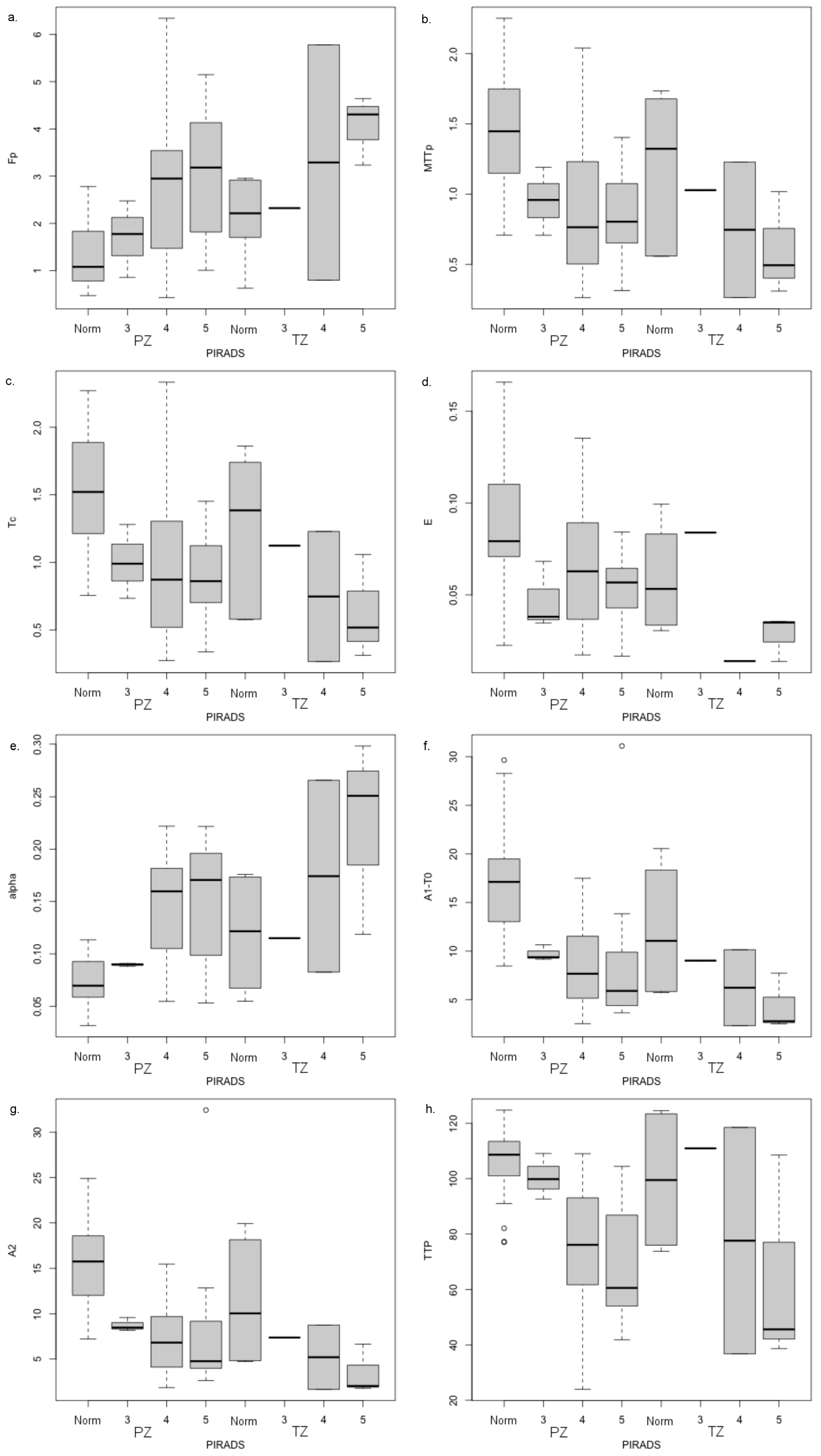
| Model | Parameter | Prostate Zone | ||
|---|---|---|---|---|
| PZ | TZ | t-Test p-Values ^ | ||
| Mean Value | ||||
| 2CU | vp | 1.761 | 1.912 | 0.684 |
| PS | 0.108 | 0.094 | 0.597 | |
| Fp | 1.363 | 2.105 | 0.0245 | |
| MTTp | 1.439 | 1.196 | 0.235 | |
| Tc | 1.534 | 1.254 | 0.195 | |
| E | 0.0861 | 0.0589 | 0.0512 | |
| Ktrans | 0.0938 | 0.0839 | 0.657 | |
| Exponential EMM | 0.0723 | 0.119 | 2.10 × 10⁻³ | |
| Sigmoidal EMM | A1 − T0 | 16.671 | 12.099 | 0.0724 |
| A2 | 15.071 | 11.287 | 0.0932 | |
| Model | Parameter | Radiological Evaluation | |
|---|---|---|---|
| ANOVA p-Values by Factor ° | |||
| Prostate Zone | PI-RADS Category | ||
| 2CU | vp | 0.866 | 0.418 |
| PS | 0.348 | 0.443 | |
| Fp | 0.403 | 2.72 × 10⁻⁵ | |
| MTTp | 0.151 | 1.45 × 10⁻⁴ | |
| Tc | 0.118 | 1.53 × 10⁻⁴ | |
| E | 0.0236 | 6.99 × 10⁻³ | |
| Ktrans | 0.374 | 0.298 | |
| Exponential EMM | 2.43 × 10⁻³ | 2.44 × 10⁻⁷ | |
| Sigmoidal EMM | A1 − T0 | 0.0264 | 4.28 × 10⁻⁶ |
| A2 | 0.0321 | 4.94 × 10⁻⁶ | |
| Curve Shape | TTP | 0.605 | 4.88 × 10⁻⁷ |
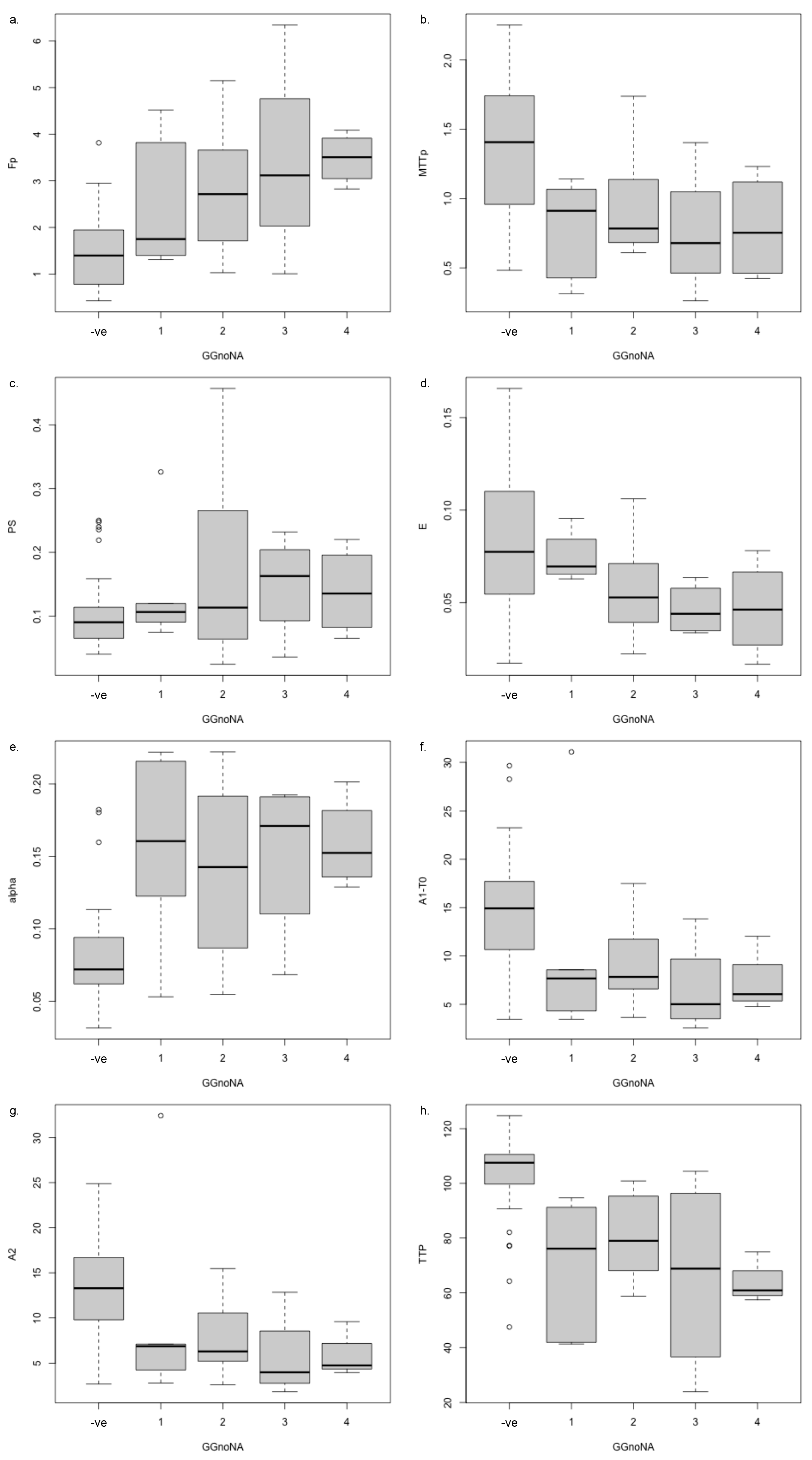
| Model | Parameter | Peripheral Zone | |
|---|---|---|---|
| Biopsy Only | Biopsy Sample + Normal-Appearing | ||
| t-Test p-Value ^ | One-Way ANOVA p-Value ° | ||
| −ve vs. +ve | −ve, GG1, GG2, GG3, GG4 | ||
| 2CU | vp | 0.355 | 0.236 |
| PS | 0.186 | 0.318 | |
| Fp | 0.0527 | 9.41 × 10⁻⁵ | |
| MTTp | 0.117 | 0.002 | |
| Tc | 0.0995 | 1.73 × 10⁻³ | |
| E | 0.391 | 0.0346 | |
| Ktrans | 0.168 | 0.234 | |
| Exponential EMM | 0.153 | 4.1 × 10⁻⁵ | |
| Sigmoidal EMM | A1 − T0 | 0.950 | 8.73 × 10⁻³ |
| A2 | 0.940 | 7.03 × 10⁻³ | |
| Curve Shape | TTP | 0.0608 | 4.72 × 10⁻⁶ |
Disclaimer/Publisher’s Note: The statements, opinions and data contained in all publications are solely those of the individual author(s) and contributor(s) and not of MDPI and/or the editor(s). MDPI and/or the editor(s) disclaim responsibility for any injury to people or property resulting from any ideas, methods, instructions or products referred to in the content. |
© 2024 by the authors. Licensee MDPI, Basel, Switzerland. This article is an open access article distributed under the terms and conditions of the Creative Commons Attribution (CC BY) license (https://creativecommons.org/licenses/by/4.0/).
Share and Cite
Clemente, A.; Selva, G.; Berks, M.; Morrone, F.; Morrone, A.A.; Aulisa, M.D.C.; Bliakharskaia, E.; De Nicola, A.; Tartaro, A.; Summers, P.E. Comparison of Early Contrast Enhancement Models in Ultrafast Dynamic Contrast-Enhanced Magnetic Resonance Imaging of Prostate Cancer. Diagnostics 2024, 14, 870. https://doi.org/10.3390/diagnostics14090870
Clemente A, Selva G, Berks M, Morrone F, Morrone AA, Aulisa MDC, Bliakharskaia E, De Nicola A, Tartaro A, Summers PE. Comparison of Early Contrast Enhancement Models in Ultrafast Dynamic Contrast-Enhanced Magnetic Resonance Imaging of Prostate Cancer. Diagnostics. 2024; 14(9):870. https://doi.org/10.3390/diagnostics14090870
Chicago/Turabian StyleClemente, Alfredo, Guerino Selva, Michael Berks, Federica Morrone, Aniello Alessandro Morrone, Michele De Cristofaro Aulisa, Ekaterina Bliakharskaia, Andrea De Nicola, Armando Tartaro, and Paul E. Summers. 2024. "Comparison of Early Contrast Enhancement Models in Ultrafast Dynamic Contrast-Enhanced Magnetic Resonance Imaging of Prostate Cancer" Diagnostics 14, no. 9: 870. https://doi.org/10.3390/diagnostics14090870