Entropy of Difference: A New Tool for Measuring Complexity

Abstract

We propose a new tool for estimating the complexity of a time series: the entropy of difference (ED). The method is based solely on the sign of the difference between neighboring values in a time series. This makes it possible to describe the signal as efficiently as prior proposed parameters, such as permutation entropy (PE) or modified permutation entropy (mPE). Firstly, this method reduces the size of the sample that is necessary to estimate the parameter value, and secondly it enables the use of the Kullback–Leibler divergence to estimate the “distance” between the time series data and random signals.

1. Introduction

Permutation entropy (PE), introduced by Bandt and Pompe [1], as well as its modified version [2], are both efficient tools for measuring the complexity of chaotic time series. Both methods propose to analyze time series $X=(x_1,x_2,\cdots x_k\cdots )$ by first choosing an embedding dimension m to split the original data in a subset of m-tuples, $((x_1,x_2\cdots x_m),$$(x_2,x_3,\cdots x_{1+m}),\cdots )$, and to then substitute the m-tuples values by the rank of the values, resulting in a new symbolic representation of the time series. For example, consider the time series $X=(0.2,0.1,0.6,0.4,0.1,0.2,0.4,0.8,0.5,1,0.3,0.1,\cdots )$. Choosing, for example, an embedding dimension $m=4$, will split the data in a set of 4-tuples: $X_4=((0.2,0.1,0.6,0.4),(0.1,0.6,0.4,0.1),(0.6,0.4,0.1,0.2),\cdots )$. The Bandt–Pompe method will associate the rank of the value with each 4-tuple. Thus, in $(0.2,0.1,0.6,0.4)$, the lowest element $0.1$ is in Position 2, the second element $0.2$ is in Position 1, $0.4$ is in Position 4, and finally $0.6$ is in Position 3. Thus, the 4-tuple $(0.2,0.1,0.6,0.4)$ is rewritten as $(2,1,4,3)$. This procedure thus results in each $X_4$ being rewritten as a symbolic list: $\left(\right(2,1,4,3),(1,4,3,2),(3,4,2,1)\cdots )$. Each element is then a permutation $\pi$ of the set $(1,2,3,4)$. Next, the probability of each permutation $\pi$ in $X_m$ is then computed, $p_m\left(\pi \right)$, and finally, the PE for the embedding dimension m is defined as ${\mathrm{PE}}_m\left(X\right)=-{\sum }_{\pi }{p}_m\left(\pi \right)log\left(p_m\left(\pi \right)\right)$. The modified permutation entropy (mPE) just deals with those cases in which equal quantities may appear in the m-tuples. For example, for the m-tuple $(0.1,0.6,0.4,0.1)$, computing PE will produce $(1,4,3,2)$, while computing mPE will associate $(1,1,3,2)$. Both methods are widely used due to their conceptual and computational simplicity [3,4,5,6,7,8]. For random signals, PE leads to a constant probability $q_m\left(\pi \right)=1/m!$ (for white Gaussian noise), which does not make it possible to evaluate the “distance” between the probability found in the signal, $p_m\left(\pi \right)$, and the probability produced by a random signal, $q_m$, with the Kullback–Leibler (KL) divergence [9,10]: ${\mathtt{KL}}_m(p\parallel q)={\sum }_{\pi }{p}_m\left(\pi \right){log}_2(p_m\left(\pi \right)/q_m\left(\pi \right))$. Furthermore, the number ${\mathtt{K}}_m$ of m-tuples is $m!$ for PE and even greater for mPE [2], thus requiring then a large data sample to perform a significant statistical estimation of $p_m$.

2. The Entropy of Difference Method

The entropy of difference (ED) method proposes to substitute the m-tuples with strings s containing the sign (“+” or “−”), representing the difference between subsequent elements in the m-tuples. For the same $X_4$, $\left(\right(0.2,0.1,0.6,0.4),$$(0.1,0.6,0.4,0.1),$$(0.6,0.4,0.1,0.2),\cdots )$ this leads to the representation (“− + −”, “+ − −”, “− − +”, ⋯). For an m value, we have $2^{m-1}$ strings s from “+ + + ⋯ +” to “− − − ⋯ −”. Again, we compute, in the time series, the probability distribution $q_m\left(s\right)$ of these strings s and define the entropy of difference of order m as ${\mathrm{ED}}_m=-{\sum }_s{q}_m\left(s\right){log}_2{q}_m\left(s\right)$. The number of elements, ${\mathtt{K}}_m$, to be treated, for an embedding m, is smaller for ED compared with the number of permutations $\pi$ in PE or to the elements in mPE (see Table 1).

Table 1. K values, for different m-embeddings.

m	3	4	5	6	7
${\mathtt{K}}_{PE}$	6	24	120	720	5040
${\mathtt{K}}_{mPE}$	13	73	501	4051	37,633
${\mathtt{K}}_{ED}$	4	8	16	32	64

Furthermore, the probability distribution for a string s, in a random signal, $q_m\left(s\right)$, is not constant and could be computed through the recursive equation. Indeed, let $P(x\le X_t\le x+dx)=p\left(x\right)dx$ be the probability density for the signal variable $X_t$ at time t, and let $F\left(x\right)$ be the corresponding cumulative distribution function ($F\left(x\right)={\int }^{x}p\left(x\right)dx$). Consider the hypothesis that the signal is not correlated in time, which means that the join probability is only the product of the probability $P(x_1\le X_{t_1}\le x_1+d{x}_1,x_2\le X_{t_2}\le x_2+d{x}_1)=P(x_1\le X_t\le x_1+d{x}_1)P(x_2\le X_t\le x_2+d{x}_2)$. Under these conditions, we can easily evaluate the $q_m\left(s\right)$. For example, $m=3$. We therefore have three data $x_1,x_2,x_3$, and we can have 4 possibilities. $q_3(+,+)$ is the probability of having $x_3>x_2>x_1$, $q_3(+,-)$ is that of having $x_2>x_1$ and $x_2>x_3$, $q_3(-,+)$ is that of having $x_1>x_2$ and $x_3>x_2$, and finally $q_3(-,-)$ is that of having $x_1>x_2>x_3$. Using the Heaviside step function $\theta \left(x\right)$, $\theta \left(x\right)=1$ if $x\ge 0$, and $\theta \left(x\right)=0$ if $x<0$, and noting the cumulative distribution function $F\left(x\right)=P(X\le x)$, we can evaluate $q_3(+,+)$:

$$\begin{array}{ccc}\hfill q_3(+,+)& =& \int \int \int d{x}_{1}d{x}_{2}d{x}_{3}p\left(x_1\right)p\left(x_2\right)p\left(x_3\right)\theta (x_3-x_2)\theta (x_2-x_1)\hfill \\ & =& \int d{x}_{3}p\left(x_3\right){\int }^{x_3}d{x}_{2}p\left(x_2\right){\int }^{x_2}d{x}_{1}p\left(x_1\right)\hfill \\ & =& \int d{x}_{3}p\left(x_3\right){\int }^{x_3}d{x}_{2}p\left(x_2\right)F\left(x_2\right)\hfill \\ & =& \int d{x}_{3}p\left(x_3\right)\frac{1}{2}F{\left(x_3\right)}^2\hfill \\ & =& \frac{1}{6}\hfill \end{array}$$

(1)

For $q_3(-,+)$, we need to integrate $\theta (x_1-x_2)\theta (x_3-x_2)$. Using the obvious $\theta (x_1-x_2)=1-\theta (x_2-x_1)$, we have

$$\begin{array}{ccc}\hfill q_3(-,+)& =& \int \int \int d{x}_{1}d{x}_{2}d{x}_{3}p\left(x_1\right)p\left(x_2\right)p\left(x_3\right)\theta (x_3-x_2)\theta (x_1-x_2)\hfill \\ & =& \int \int d{x}_{2}d{x}_{3}p\left(x_2\right)p\left(x_3\right)\theta (x_3-x_2)-q_3(+,+)\hfill \\ & =& \int d{x}_{3}p\left(x_3\right)F\left(x_3\right)-\frac{1}{6}=\int d{x}_3{F}^{\prime }\left(x_3\right)F\left(x_3\right)-\frac{1}{6}\hfill \\ & =& \frac{1}{2}-\frac{1}{6}=\frac{2}{6}\hfill \end{array}$$

(2)

This result is totally independent of the probability density $p\left(x\right)$ provided that the signal is not correlated in time. We can proceed in the same way for any $q_m\left(s\right)$ and thus obtain a recurrence on $q_m\left(s\right)$ (see Appendix A) (in the following equations, x and y are strings made of “+” and “−”):

$$\begin{array}{c}\hfill q_2(+)=q_2(-)=\frac{1}{2}\\ \hfill q_{m+1}(\underset{m}{\underbrace{+,+,+,\cdots ,+}})=\frac{1}{(m+1)!}\\ \hfill q_{m+1}(-,\mathrm{x})=q_m\left(\mathrm{x}\right)-q_{m+1}(+,\mathrm{x})\\ \hfill q_{m+1}(\mathrm{x},-)=q_m\left(\mathrm{x}\right)-q_{m+1}(\mathrm{x},+)\\ \hfill q_{m+1}(\mathrm{x},-,\mathrm{y})=q_{a+1}\left(\mathrm{x}\right)q_{b+1}\left(\mathrm{y}\right)-q_{m+1}(\mathrm{x},+,\mathrm{y})\mathrm{with}a+b+1=m\end{array}$$

(3)

leading to a complex probability distribution for $q_m\left(s\right)$. For example, for $m=9$, we have $2^8=256$ strings with the highest probability for the “+ − + − + − + −” string (and its symmetric “− + − + − + − +”): $q_9\left(\max \right)=\frac{62}{2835}\approx 0.02187$ (see Figure 1). These probabilities $q_m\left(s\right)$ could then be used to determine the KL-divergence between the time series probability $p_m\left(s\right)$ and the random uncorrelated signal.

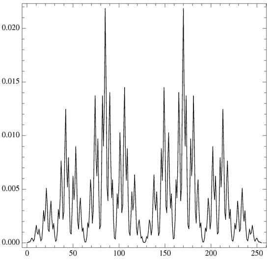
Figure 1. The $2^8$ values for the probability of $q_9\left(s\right)$, from $s=---\dots \equiv 0$ to $s=+++\dots \equiv 255$.

To each string s, we can associate an integer number, its binary representation, through the substitutions $-\to 0$ and $+\to 1$. Therefore, for $m=4$, we have “− − −” = 0, “− − +” = 1, “− + −” = 2, “− + +” = 3, and so on, up to “+ + +” = 7 (see Table 2 and Table 3).

Table 2. $q_m$ values, for different m-embeddings, ordered by the binary representation of the string.

$s=$	0	1	2	3	4	5	6	7	8	9	10	11	12	13	14	15
$6q_3=$	1	2	2	1
$24q_4=$	1	3	5	3	3	5	3	1
$120q_5=$	1	4	9	6	9	16	11	4	4	11	16	9	6	9	4	1

Table 3. ${\mathrm{ED}}_m$ values, for different m-embeddings.

${\mathrm{ED}}_2=$	1
${\mathrm{ED}}_3=$	$\frac{1}{3}+{log}_2\left(3\right)=1.9183$
${\mathrm{ED}}_4=$	$3+\frac{1}{2}{log}_2\left(3\right)-\frac{5}{12}{log}_2\left(5\right)=2.82501$
${\mathrm{ED}}_5=$	$\frac{47}{30}+\frac{3}{10}{log}_2\left(3\right)+{log}_2\left(5\right)-\frac{11}{60}{log}_2\left(11\right)=3.72985$

The recurrence gives some specific $q_m$. To simplify the notations, we can write $a_{+}$, a set of a successive “+”. For example, the second and third rules gives

$$\begin{array}{ccc}& q_{m+1}(a_{+},-)& =q_m\left(a_{+}\right)-q_{m+1}(a_{+},+)=\frac{1}{m!}-\frac{1}{(m+1)!}\hfill \\ & q_{m+1}(a_{+},-)& =q_{m+1}(-,a_{+})=\frac{m}{(m+1)!}\hfill \end{array}$$

(4)

then

$$\begin{array}{ccc}& q_{m+1}(a_{+},-,b_{+})& =q_{a+1}\left(a_{+}\right)q_{b+1}\left(b_{+}\right)-q_{m+1}(a_{+},+,b_{+})=\hfill \\ & q_{m+1}(a_{+},-,b_{+})& =\frac{1}{(m+1)!}\left(C_{a+1}^{m+1}-1\right)\mathrm{with}:b+a+1=m\hfill \end{array}$$

(5)

We can also write

$$\begin{array}{c}\hfill q_{m+1}(a_{+},-,b_{+},-,c_{+})=q_{a+1}\left(a_{+}\right)q_{b+c+2}(b_{+},-,c_{+})-q_{m+1}(a_{+},+,b_{+},-,c_{+})=\\ \hfill a+b+c+2=m\\ \hfill q_{m+1}(a_{+},-,b_{+},-,c_{+})=\frac{1}{(a+1)!}\frac{1}{(m-a)!}\left(C_{b+1}^{m-a}-1\right)-\frac{1}{(m+1)!}\left(C_{m-c}^{m+1}-1\right)=\\ \hfill =\frac{1}{(a+1)!(b+1)!(c+1)!}-\frac{1}{(c+1)!(a+b+2)!}-\frac{1}{(a+1)!(b+c+2)!}+\frac{1}{(a+b+c+3)!}\end{array}$$

(6)

This equation is also valid when $b=0$ and thus for $q_{m+1}(a_{+},-,-,c_{+})$ (with $m=a+c+2$) or for $c=0$. We can continue in this way and determine the general values of $q_{m+1}(a_{+},-,b_{+},-,c_{+},-,d_{+})$ and so on.

In the case, where the data are integers, we can avoid the situation where two successive data are equal ($x_i=x_{i+1}$) by adding a small amount of random noise. For example, we take the first ${10}^4$ decimal of $\pi$ (and we add a small amount of noise $ϵ\in [-0.01,0.01]$), and we have the following (See Table 4 and Table 5):

Table 4. $q_m$ values for $\pi$, for different m-embeddings.

$6q_3=$	0.982	2.01	2.01	0.991
$24q_4=$	0.924	3.00	5.05	3.00	3.00	5.05	3.00	0.960
$120q_5=$	0.756	3.86	9.10	5.92	9.23	16.0	11.0	4.03	3.86	11.1	16.2	9.10
	5.78	9.22	4.03	0.768

Table 5. ${\mathrm{ED}}_m$ values for $\pi$, for different m-embeddings.

${\mathrm{ED}}_2=$	0.999998
${\mathrm{ED}}_3=$	1.91361
${\mathrm{ED}}_4=$	2.81364
${\mathrm{ED}}_5=$	3.71059

Despite the complexity of $q_m\left(s\right)$, the Shannon entropy for a random signal, ${\mathrm{ED}}_m=-{\sum }_s{q}_m\left(s\right){log}_2{q}_m\left(s\right)$, increases linearly with m (see Figure 2): ${\mathrm{ED}}_m=-0.799574+0.905206m$. If the m-tuples are equiprobable, it will lead to $-{log}_2\left(2\right)+m{log}_2\left(2\right)=m-1$.

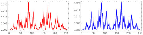
Figure 2. The $2^8$ values for the probability of $q_9\left(s\right)$, for the $\pi$ decimal (blue), and for a random distribution (red).

3. Periodic Signal

We will now see what happens with a period 3 data $X=(x_1,x_2,x_3,x_1,x_2,x_3,\cdots )$. To evaluate $q_m$, we only have 3 types of 2-tuples. For example, for $q_2$, we have $((x_1,x_2)$, $(x_2,x_3)$, and $(x_3,x_1))$. We have only two possible strings, “+” or “−”, so the probabilities must be $q_2(+)=2/3,q_2(-)=1/3$ or $q_2(+)=1/3,q_2(-)=2/3$. For $q_3$, again we have only 3 types of 3-tuples: $((x_1,x_2,x_3)$, $(x_2,x_3,x_1)$, and $(x_3,x_1,x_2))$. We have $2^2$ possible strings $(+,+)$, $(+,-)$, $(-,+)$, and $(-,-)$. The consistency of the inequalities between $x_1$, $x_2$, and $x_3$ reduces the number of possible strings to 3. For example, if $(x_1,x_2,x_3)$ gives $(+,+)$, then $(x_2,x_3,x_1)$ must be $(+,-)$, and $(x_3,x_1,x_2)$ must be $(-,+)$. Due to Period 3, these $\left(\mathtt{x},\mathtt{y}\right)$ values will appear $1/3$ times. To evaluate $q_4$, we have again only 3 types of 4-tuples: $((x_1,x_2,x_3,x_1)$, $(x_2,x_3,x_1,x_2)$, and $(x_3,x_1,x_2,x_3))$, and again these will appear $1/3$ times in the data. This reasoning can be generalized to a signal of period p, $q_p=1/p$; consequently, ${\mathrm{ED}}_p={log}_2\left(p\right)$, and this remains constant for $m\ge p$. Obviously, since we are only using the differences between the $x_i$’s, the periodicity in terms of signs $x_{i+1}-x_i$ may be smaller than the periodicity p of the data, so ${\mathrm{ED}}_p\le {log}_2\left(p\right)$.

4. Chaotic Logistic Map Example

Let us illustrate the use of ED on the well known logistic map [11] $\mathtt{Lo}(x,\lambda )$ driven by the parameter $\lambda$.

$$x_{n+1}=\mathtt{Lo}(x_n,\lambda )=\lambda x_n(1-x_n)$$

(7)

It is obvious that, for a range of values of $\lambda$, where the time series reaches a periodic behavior (any cyclic oscillation between n different values), the ED will remain constant. The evaluation of the ED could thus be used as a new complexity parameter to determine the behavior of the time series (see Figure 3).

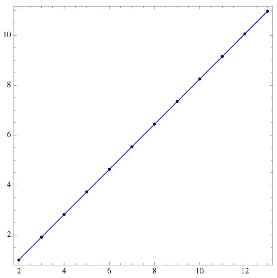
Figure 3. The Shannon entropy of $q_m\left(s\right)$: ${\mathrm{ED}}_m$ increases linearly with m, and the fit $-0.799574+0.905206m$ gives a sum of squared residuals of $1.7\times {10}^{-4}$ and a p-value = $1.57\times {10}^{-12}$ and $1.62\times {10}^{-30}$ on the fit parameter respectively.

For $\lambda =4$, we know that the data are randomly distributed with a probability density given by [12]

$$p_{\mathtt{Lo}}\left(x\right)=\frac{1}{\pi \sqrt{(1-x)x}}$$

(8)

However, the logistic map produces correlations in the data, so we expect a deviation from the uncorrelated random $q_m$.

We can then compute exactly the ED for an m-embedding as well as the KL-divergence from a random signal. For example, for $m=2$, we can determine $q_2^{\mathtt{Lo}}(+)$ and $q_2^{\mathtt{Lo}}(-)$ by solving the inequality $x<\mathtt{Lo}\left(x\right)$ and $x>\mathtt{Lo}\left(x\right)$, respectively, which implies that $0<x<3/4$ and $3/4<x<1$. Then,

$$q_2^{\mathtt{Lo}}(+)={\int }_0^{3/4}dx{p}_{\mathtt{Lo}}\left(x\right)=\frac{2}{3}{q}_2^{\mathtt{Lo}}(-)={\int }_{3/4}^{1}dx{p}_{\mathtt{Lo}}\left(x\right)=\frac{1}{3}$$

(9)

In this case, the logistic map produces a signal that contains twice as many increasing pairs “+” than decreasing pairs “−”. Thus,

$${\mathrm{ED}}_2=-(\frac{2}{3}{log}_2\frac{2}{3}+\frac{1}{3}{log}_2\frac{1}{3})={log}_2\frac{3}{2^{2/3}}\approx 0.918{\mathtt{KL}}_2=\frac{1}{3}{log}_2\frac{32}{27}\approx 0.082$$

(10)

For $m=3$, we can perform the same calculation. We have, respectively,

$$\begin{array}{ccc}\hfill x_1<x_2<x_3& \to & (+,+):0<x<\frac{1}{4}\hfill \\ \hfill x_1<x_3<x_2& \to & (+,-):\frac{1}{4}<x<\frac{1}{8}(5-\sqrt{5})\hfill \\ \hfill x_3<x_1<x_2& \to & (+,-):\frac{1}{8}(5-\sqrt{5})<x<\frac{3}{4}\hfill \\ \hfill x_2<x_1<x_3& \to & (-,+):\frac{3}{4}<x<\frac{1}{8}(5+\sqrt{5})\hfill \\ \hfill x_2<x_3<x_1& \to & (-,+):\frac{1}{8}(5+\sqrt{5})<x<1\hfill \end{array}$$

Graphically we have:

$$\begin{array}{c}\hfill q_3^{\mathtt{Lo}}(++)=\frac{1}{3}{q}_3^{\mathtt{Lo}}(+-)=\frac{1}{3}{q}_3^{\mathtt{Lo}}(-+)=\frac{1}{3}{q}_3^{\mathtt{Lo}}(--)=0\\ \hfill \to {\mathrm{ED}}_3={log}_{2}3\approx 1.58{\mathtt{KL}}_3=\frac{1}{3}\approx 0.33\end{array}$$

(11)

Effectively, the logistic map with $\lambda =4$ forbids the string “$--$” where $x_1>x_2>x_3$. For strings of length 3, we have

$$\begin{array}{c}\hfill q_4^{\mathtt{Lo}}(+++)=q_4^{\mathtt{Lo}}(++-)=q_4^{\mathtt{Lo}}(-++)=q_4^{\mathtt{Lo}}(-+-)=\frac{1}{6}{q}_4^{\mathtt{Lo}}(+-+)=\frac{2}{6}\\ \hfill \to {\mathrm{ED}}_4={log}_2{108}^{\frac{1}{3}}\approx 2.25{\mathtt{KL}}_4={log}_2{\left(\frac{16,384}{1125}\right)}^{1/6}\approx 0.64\end{array}$$

(12)

The probability of difference $q_m\left(s\right)$ for some string length m versus s, the string binary value, where “+”$\to 1$ and “−”$\to 0$, gives us the “spectrum of difference” for the distribution q (see Figure 4 and Figure 5).

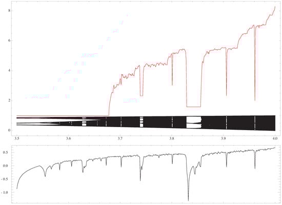
Figure 4. The ${\mathrm{ED}}_{13}$ (strings of length 12) is plotted versus $\lambda$, with the bifurcation diagram, and the value of the Lyapunov exponent, respectively [13]. The constant value appears when the logistic map enters into a periodic regime.

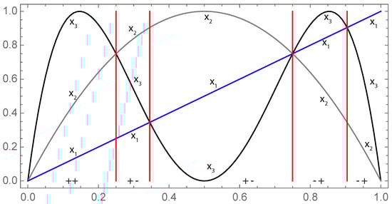
Figure 5. From $x_1$ (blue), the first iteration of the logistic map (gray) gives $x_2$, and the second iteration (black) gives $x_2$. The respective positions of $x_1,x_2,x_3$ allow us to determine $q_3$.

5. KL_m(p|q) Divergences Versus m on Real Data and on Maps

The manner in which the ${\mathtt{KL}}_m\left(p\right|q)$ evolves with m is another parameter of the complexity measure. ${\mathtt{KL}}_m\left(p\right|q)$ measures the loss of information when the random distribution $q_m$ is used to predict the distribution $p_m$. Increasing m introduces more bits of information in the signal, and the behavior versus m shows how the data diverge from a random distribution.

The graphics (see Figure 6) show the behavior of ${\mathtt{KL}}_m$ versus m for two different chaotic maps and for real financial data [14]: the opening value of the nasdaq100, bel20 every day from 2000 to 2013. For maps, the logarithmic map $x_{n+1}=ln\left(a\right|x_n\left|\right)$ and the logistic map are shown (see Figure 6 for the logarithmic map (Figure 7)).

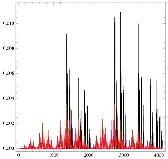
Figure 6. The spectrum of $q_{13}^{\mathtt{Lo}}$ (black) versus the string binary value (from 0 to $2^{12}-1$) for the logistic map at $\lambda =4$ and the one from a random distribution $q_{13}$ (red).

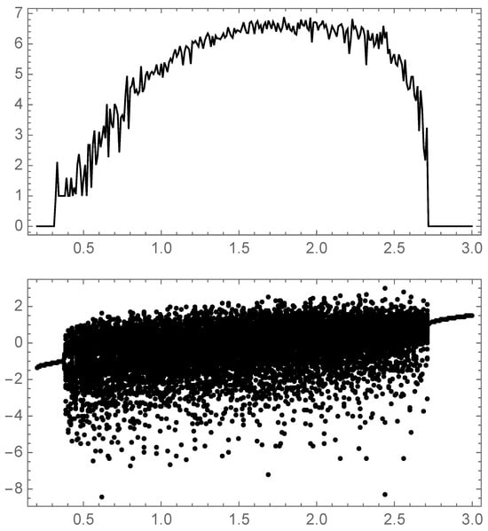
Figure 7. The ${\mathrm{ED}}_{13}$ versus a for the logarithm map $x_{n+1}=ln\left(a\right|x_n\left|\right)$.

For maps, the simulation starts with a random number between 0 and 1 and first iterates 500 times to avoid transients. Starting with these seeds, 720 iterates were kept, and ${\mathtt{KL}}_m$ was computed. It can be seen that the Kullback–Leibler divergence from the logistic map at $\lambda =4$ to the random signal is fitted by a quadratic function of m: ${\mathtt{KL}}_m=-0.4260+0.2326m+0.0095m^2$ (p-value $\approx 2\times {10}^{-7}$ for all parameters), while the logarithmic map behavior is linear in the range $a\in [0.4,2.2]$. Financial data are also quadratic ${\mathtt{KL}}_m\left(\mathrm{nasdaq}\right)=0.1824-0.0973m+0.0178m^2$, ${\mathtt{KL}}_m\left(\mathrm{bel}20\right)=0.1587-0.0886m+0.0182m^2$ with a higher curvature than the logistic map due to the fact that the spectrum of the probability $p_m$ is compatible with a constant distribution (see Figure 6), rendering the prediction of an increase or decrease signal completely random, which is not the case in any true random signal (See Figure 8 and Figure 9).

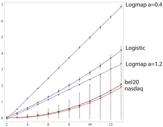
Figure 8. The KL-divergence for the data.

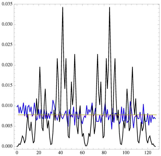
Figure 9. The spectrum of $q_8$ versus the string binary value (from 0 to $2^7-1$) for the bel20 financial data.

6. Conclusions

The simple property of increases or decreases in a signal makes it possible to introduce the entropy of difference ${\mathrm{ED}}_m$ as a new efficient complexity measure for chaotic time series. This new technique is numerically fast and easy to implement. It does not require complex signal processing and could replace the evaluation of the Lyapunov exponent (which is far more time-consuming). For a random signal, we have determined the value of ${\mathrm{ED}}_m$, which is independent of the probability of distribution of this signal. This makes it possible to calculate the “distance” between the analyzed signal and a random signal (independent of its distribution probability). As “distance”, we evaluate the Kullback–Leibler divergence versus the number of data m used to build the difference string. This ${\mathtt{KL}}_m$ shows different behavior for different types of signal and can also be used also to characterize the complexity of a time series. Since the only assumption for a random signal is that it is uncorrelated, this method makes it possible to determine the correlated nature of signals, even in chaotic regimes.

References

- Bandt, C.; Pompe, B. Permutation Entropy: A Natural Complexity Measure for Time Series. Phys. Rev. Lett. 2002, 88, 174102. [Google Scholar] [CrossRef]
- Bian, C.; Qin, C.; Ma, Q.D.Y.; Shen, Q. Modified permutation-entropy analysis of heartbeat dynamics. Phys. Rev. E 2012, 85, 021906. [Google Scholar] [CrossRef]
- Zunino, L.; Pérez, D.G.; Martín, M.T.; Garavaglia, M.; Plastino, A.; Rosso, O.A. Permutation entropy of fractional Brownian motion and fractional Gaussian noise. Phys. Lett. A 2008, 372, 4768. [Google Scholar] [CrossRef]
- Li, X.; Ouyang, G.; Richard, D.A. Predictability analysis of absence seizures with permutation entropy. Epilepsy Res. 2007, 77, 70. [Google Scholar] [CrossRef]
- Li, X.; Cui, S.; Voss, L.J. Using permutation entropy to measure the electroencephalographic effects of sevoflurane. Anesthesiology 2008, 109, 448. [Google Scholar] [CrossRef] [PubMed]
- Frank, B.; Pompe, B.; Schneider, U.; Hoyer, D. Permutation entropy improves fetal behavioural state classification based on heart rate analysis from biomagnetic recordings in near term fetuses. Med. Biol. Eng. Comput. 2006, 44, 179. [Google Scholar] [CrossRef] [PubMed]
- Olofsen, E.; Sleigh, J.W.; Dahan, A. Permutation entropy of the electroencephalogram: A measure of anaesthetic drug effect. Br. J. Anaesth. 2008, 101, 810. [Google Scholar] [CrossRef] [PubMed]
- Rosso, O.A.; Zunino, L.; Perez, D.G.; Figliola, A.; Larrondo, H.A.; Garavaglia, M.; Martin, M.T.; Plastino, A. Extracting features of Gaussian self-similar stochastic processes via the Bandt–Pompe approach. Phys. Rev. E 2007, 76, 061114. [Google Scholar] [CrossRef] [PubMed]
- Kullback, S.; Leibler, R.A. On Information and Sufficiency. Ann. Math. Statist. 1951, 22, 79. [Google Scholar] [CrossRef]
- Roldán, E.; Parrondo, J.M.R. Entropy production and Kullback–Leibler divergence between stationary trajectories of discrete systems. Phys. Rev. E 2012, 85, 031129. [Google Scholar] [CrossRef] [PubMed]
- May, R.M. Simple mathematical models with very complicated dynamics. Nature 1976, 261, 459. [Google Scholar] [CrossRef] [PubMed]
- Jakobson, M. Absolutely continuous invariant measures for one-parameter families of one-dimensional maps. Commun. Math. Phys. 1981, 81, 39–88. [Google Scholar] [CrossRef]
- Ginelli, F.; Poggi, P.; Turchi, A.; Chate, H.; Livi, R.; Politi, A. Characterizing Dynamics with Covariant Lyapunov Vectors. Phys. Rev. Lett. 2007, 99, 130601. [Google Scholar] [CrossRef] [PubMed]
- Available online: http://www.wessa.net/ (accessed on 1 February 2024).
Disclaimer/Publisher’s Note: The statements, opinions and data contained in all publications are solely those of the individual author(s) and contributor(s) and not of MDPI and/or the editor(s). MDPI and/or the editor(s) disclaim responsibility for any injury to people or property resulting from any ideas, methods, instructions or products referred to in the content. |
© 2024 by the authors. Licensee MDPI, Basel, Switzerland. This article is an open access article distributed under the terms and conditions of the Creative Commons Attribution (CC BY) license (https://creativecommons.org/licenses/by/4.0/).