Vector-Valued Shepard Processes: Approximation with Summability

Abstract

In this work, vector-valued continuous functions are approximated uniformly on the unit hypercube by Shepard operators. If $\lambda$ denotes the usual parameter of the Shepard operators and m is the dimension of the hypercube, then our results show that it is possible to obtain a uniform approximation of a continuous vector-valued function by these operators when $\lambda \ge m+1$. By using three-dimensional parametric plots, we illustrate this uniform approximation for some vector-valued functions. Finally, the influence in approximation by regular summability processes is studied, and their motivation is shown.

1. Introduction

The Shepard operators, initially defined by Donald Shepard in 1968 [1], are effectively employed in a wide array of fields, ranging from mathematics to engineering, and from geographical mapping systems to mining, owing to their interpolation capabilities as well as their ability to approximate functions more rapidly. These operators are quite successful not only in scattered data interpolation problems (see [2,3,4,5,6,7,8]) but also in the classical approximation theory (see [9,10,11,12,13,14,15]). Recently in [16,17], we investigated the approximation behavior of the Shepard operators in complex cases. Our main focus in this paper is to use these operators to approximate vector-valued functions on the unit hypercube and further enhance this approach through the utilization of regular summability methods.

Firstly, let us introduce the vector-valued Shepard operators that will be employed throughout this article.

Let $m\in \mathbb{N}$ and $\mathbf{K}$ be the unit hypercube (or, the unit m-dimensional square), i.e.,

$$\mathbf{K}={[0,1]}^m=\left\{\mathbf{x}=(x_1,x_2,\dots ,x_m)\in {\mathbb{R}}^m:x_i\in [0,1],i=1,2,\dots ,m\right\}.$$

Fixed $n\in \mathbb{N}$, examine the set given by

$${\Omega }_n:=\left\{\mathbf{k}=(k_1,k_2,\dots ,k_m)\in {\mathbb{N}}^m:k_i\in \{0,1,\dots ,n\},i=1,2,\dots ,m\right\}$$

and the following sample points of $\mathbf{K}$

$${\mathbf{x}}_{\mathbf{k},n}=\left(\frac{k_1}{n},\frac{k_2}{n},\dots ,\frac{k_m}{n}\right)\mathrm{with}\mathbf{k}\in {\Omega }_n.$$

Then, in total, we have ${(n+1)}^m$ sample points on $\mathbf{K}$. Assume $d\in \mathbb{N}$ and $\mathbf{f}=(f_1,f_2,\dots ,f_d)$ is a vector-valued function on the set $\mathbf{K}$, where each component $f_r$$(r=1,2,\dots ,d)$ is a real-valued function on the set $\mathbf{K}$. Now, if $0<\lambda \in \mathbb{R}$, we examine the following vector-valued Shepard processes:

$${\mathbb{S}}_{n,\lambda }(\mathbf{f};\mathbf{x})=\frac{{\sum }_{\mathbf{k}=\mathbf{0}}^n{\left|\mathbf{x}-{\mathbf{x}}_{\mathbf{k},n}\right|}_m^{-\lambda }\mathbf{f}\left({\mathbf{x}}_{\mathbf{k},n}\right)}{{\sum }_{\mathbf{k}=\mathbf{0}}^n{\left|\mathbf{x}-{\mathbf{x}}_{\mathbf{k},n}\right|}_m^{-\lambda }},$$

(1)

where we write ${\sum }_{\mathbf{k}=\mathbf{0}}^n$ for the multi-index summation ${\sum }_{k_1=0}^n{\sum }_{k_2=0}^n\cdots {\sum }_{k_m=0}^n$. Here, the symbol ${\left|·\right|}_m$ denotes the usual Euclidean norm on the set $\mathbf{K}$. Observe that ${\mathbb{S}}_{n,\lambda }\left(\mathbf{f}\right)$ is an interpolatory process at the sample points ${\mathbf{x}}_{\mathbf{k},n},$ i.e.,

$${\mathbb{S}}_{n,\lambda }(\mathbf{f};{\mathbf{x}}_{\mathbf{k},n})=\mathbf{f}\left({\mathbf{x}}_{\mathbf{k},n}\right)\mathrm{for}\mathbf{k}\in {\Omega }_n.$$

It is easy to verify that ${\mathbb{S}}_{n,\lambda }\left(\mathbf{f}\right)$ may be written with respect to the components of $\mathbf{f}$ as follows:

$${\mathbb{S}}_{n,\lambda }(\mathbf{f};\mathbf{x})=\left({\tilde{\mathbb{S}}}_{n,\lambda }(f_1;\mathbf{x}),{\tilde{\mathbb{S}}}_{n,\lambda }(f_2;\mathbf{x}),\dots ,{\tilde{\mathbb{S}}}_{n,\lambda }(f_d;\mathbf{x})\right),$$

where ${\tilde{\mathbb{S}}}_{n,\lambda }$ is given by

$${\tilde{\mathbb{S}}}_{n,\lambda }(g;\mathbf{x}):=\frac{{\sum }_{\mathbf{k}=\mathbf{0}}^n{\left|\mathbf{x}-{\mathbf{x}}_{\mathbf{k},n}\right|}_m^{-\lambda }g\left({\mathbf{x}}_{\mathbf{k},n}\right)}{{\sum }_{\mathbf{k}=\mathbf{0}}^n{\left|\mathbf{x}-{\mathbf{x}}_{\mathbf{k},n}\right|}_m^{-\lambda }}$$

(2)

for real-valued functions g defined on $\mathbf{K}$. It is clear that ${\tilde{\mathbb{S}}}_{n,\lambda }(g;\mathbf{x})$ becomes real valued.

We structure the present paper based on this terminology as follows: Section 2 examines the approximation characteristics of the vector-valued Shepard operators, employing both classical convergence and regular summability methods. Section 3 demonstrates our main approximation theorem through supporting the auxiliary results. Section 4 gives some significant applications, including the influence in approximating by regular summability processes. The last section is devoted to the concluding remarks.

2. Approximating by Vector-Valued Shepard Operators

Let $C(\mathbf{K},{\mathbb{R}}^d)$ denote the space of all continuous functions from $\mathbf{K}$ into ${\mathbb{R}}^d$. Now, we state an approximation result for the vector-valued Shepard operators given by (1).

Theorem 1.

Let $f\in C(\mathbf{K},{\mathbb{R}}^d)$. If $\lambda \ge m+1$, we obtain

$${\mathbb{S}}_{n,\lambda }\left(\mathbf{f}\right)\rightrightarrows \mathbf{f}on\mathbf{K},$$

(3)

with ⇉ denoting the uniform convergence.

Note that the uniform convergence in (3) can be written explicitly with respect to the components of $\mathbf{f}:$

$$\begin{array}{cc}\hfill {\mathbb{S}}_{n,\lambda }\left(\mathbf{f}\right)\rightrightarrows \mathbf{f}\mathrm{on}\mathbf{K}& \iff \mathrm{for}\mathrm{each}r=1,2,\dots ,d,\underset{n\to \infty }{lim}∥{\tilde{\mathbb{S}}}_{n,\lambda }\left(f_r\right)-f_r∥=0\hfill \\ \hfill & \iff \mathrm{for}\mathrm{each}r=1,2,\dots ,d,\underset{n\to \infty }{lim}\left\{\underset{\mathbf{x}\in \mathbf{K}}{sup}\left|{\tilde{\mathbb{S}}}_{n,\lambda }(f_r;\mathbf{x})-f_r\left(\mathbf{x}\right)\right|\right\}=0.\hfill \end{array}$$

Remark 1.

We should note that Farwig in [8] considered the multidimensional Shepard operators by using n distinct sample points in a compact set A satisfying two conditions of regularity. However, in (1), taking ${(n+1)}^m$ sample points in the unit hypercube $\mathbf{K}$, we consider not only multidimensional but also vector-valued Shepard operators. One can also check that if we take $d=1$ in Theorem 1, then our approximation result is in agreement with Farwig’s theorem in [8]. Indeed, it follows from Theorem 2.3 in [8] (in accordance with our notations, take $q=0$, $r=1/n$, $s=m$, $p=\lambda$) that the order of approximation is $O\left(\right(logn)/n)$ when $\lambda =m+1$ and $O(1/n)$ when $\lambda >m+1$, which coincides with our Theorem 1. Here, we will examine the demonstration of Theorem 1 from a different point of view than Farwig’s method (see Section 3). However, unlike Farwig’s result, we have not yet proved the existence of the approximation when $m\le \lambda <m+1$. We also give some applications that graphically and numerically illustrate the approximation of some vector-valued functions (see Section 4).

We now discuss the effects of the regular summability methods to the approximation in Theorem 1. We first recall some preliminaries on summability. Let A be a matrix $A:=\left[a_{jn}\right]$$\left(j,n\in \mathbb{N}\right)$ and x a sequence $x:=\left\{x_n\right\}$. Then, for the A-transformed sequence of $\left\{x_n\right\}$, we write $Ax:=\left\{{\left(Ax\right)}_j\right\}={\sum }_{n=1}^{\infty }{a}_{jn}{x}_n$, if we obtain convergence for the series, at each j. In such a case, we write A as a summability (matrix) method. If $limAx=L$, with $L\in R,$ for the sequence $x=\left\{x_n\right\},$ this sequence is said to be A-summable (or A-convergent) to L (we write A-lim $x=L$). For a vector-valued functions sequence, this limit can also be considered. Examine the function sequence $\left\{{\mathbf{f}}_n\right\}=\left\{(f_{1,n},f_{2,n},\dots ,f_{d,n})\right\}$. One says $\left\{{\mathbf{f}}_n\right\}$ is (uniformly) A-summable to $\mathbf{f}=(f_{1,n},f_{2,n},\dots ,f_{d,n})$ on $\mathbf{K}$ if

$$\sum _{n=1}^{\infty }{a}_{jn}{\mathbf{f}}_n\rightrightarrows \mathbf{f}\mathrm{on}\mathbf{K}$$

or, equivalently, for each $r=1,2,\dots ,d$,

$$\sum _{n=1}^{\infty }{a}_{jn}{f}_{r,n}\rightrightarrows f_r\mathrm{on}\mathbf{K},$$

which is denoted by ${\mathbf{f}}_n\stackrel{A}{\rightrightarrows }\mathbf{f}$ on $\mathbf{K}.$ We also write that a matrix summability method A is regular when A-lim $x=L$, if $limx=L.$ By using the well-known Silverman–Toeplitz result (see, for instance, [18,19]), one can characterize the regularity of a matrix summability method as follows:

$$A=\left[a_{jn}\right]\mathrm{is}\mathrm{regular}\iff \left\{\begin{array}{c}\underset{n\to \infty }{lim}{a}_{jn}=0\mathrm{for}\mathrm{every}j,\hfill \\ \underset{j\to \infty }{lim}{\displaystyle \sum _{n=1}^{\infty }}{a}_{jn}=1,\hfill \\ \underset{j\in \mathbb{N}}{sup}{\displaystyle \sum _{n=1}^{\infty }}\left|a_{jn}\right|<\infty .\hfill \end{array}\right.$$

(4)

A summability method $A=\left[a_{jn}\right]$ is said to be non-negative if $a_{jn}\ge 0$ for all $j,n\in \mathbb{N}$. We should note that non-negative regular summability processes are successful in approximation theory (cfr. [20,21,22,23,24,25,26]). Now we apply such methods in approximating by vector-valued Shepard operators.

From Theorem 1, we deduce that, for each $f\in C(\mathbf{K},{\mathbb{R}}^d)$ and $\lambda \ge m+1,$

$${\mathbb{S}}_{n,\lambda }\left(\mathbf{f}\right)\rightrightarrows \mathbf{f}\mathrm{on}\mathbf{K}.$$

(5)

Now, for a fixed non-negative regular summability method $A=\left[a_{jn}\right]$, we immediately check that, for every $\lambda \ge m+1$,

$${\mathbb{S}}_{n,\lambda }\left(\mathbf{f}\right)\stackrel{A}{\rightrightarrows }\mathbf{f}\mathrm{on}\mathbf{K},$$

provided that the transformed operator ${\sum }_{n=1}^{\infty }{a}_{jn}{\mathbb{S}}_{n,\lambda }\left(\mathbf{f}\right)$ is well defined for each j. Indeed, we may write from (1), (4) and (5), for each $r=1,2,\dots ,d$,

$$∥\sum _{n=1}^{\infty }{a}_{jn}{\tilde{\mathbb{S}}}_{n,\lambda }\left(f_r\right)-f_r∥\le \sum _{n=1}^{\infty }{a}_{jn}∥{\tilde{\mathbb{S}}}_{n,\lambda }\left(f_r\right)-f_r∥+∥f_r∥\left|\sum _{n=1}^{\infty }{a}_{jn}-1\right|\to 0,\mathrm{as}j\to \infty ,$$

since $A=\left[a_{jn}\right]$ is non-negative and regular. However, the next modifications give a motivation for regular summability methods in approximating processes.

Assume that, for each $n\in \mathbb{N}$, ${\mathbf{u}}_n:\mathbf{K}\to {\mathbb{R}}^d$ and ${\mathbf{v}}_n:\mathbf{K}\to \mathbf{K}$ are vector-valued functions such that

$${\mathbf{u}}_n=\left(u_{1,n},u_{2,n},\dots ,u_{d,n}\right)$$

and

$${\mathbf{v}}_n=\left(v_{1,n},v_{2,n},\dots ,v_{m,n}\right)$$

have bounded components on $\mathbf{K}$. Using the sequences $\left\{{\mathbf{u}}_n\right\}$ and $\left\{{\mathbf{v}}_n\right\}$, we consider the following modifications of vector-valued Shepard operators:

$${\mathbb{S}}_{n,\lambda }^{\ast }(\mathbf{f};\mathbf{x})=\left(u_{1,n}\left(\mathbf{x}\right){\tilde{\mathbb{S}}}_{n,\lambda }\left(f_1;\mathbf{x}\right),\dots ,u_{d,n}\left(\mathbf{x}\right){\tilde{\mathbb{S}}}_{n,\lambda }\left(f_d;\mathbf{x}\right)\right)$$

(6)

and

$${\mathbb{S}}_{n,\lambda }^{\ast \ast }(\mathbf{f};\mathbf{x})=\left({\tilde{\mathbb{S}}}_{n,\lambda }\left(f_1;{\mathbf{v}}_n\left(\mathbf{x}\right)\right),\dots ,{\tilde{\mathbb{S}}}_{n,\lambda }\left(f_d;{\mathbf{v}}_n\left(\mathbf{x}\right)\right)\right)$$

(7)

for $\mathbf{x}\in \mathbf{K}$, if $n\in \mathbb{N}$, $\lambda >0$ and $\mathbf{f}\in C(\mathbf{K},{\mathbb{R}}^d).$ Introducing the vector-valued test functions

$${\mathbf{e}}_0:\mathbf{K}\to {\mathbb{R}}^d,e_0\left(\mathbf{x}\right)=\mathbf{1}=(1,1,\dots ,1)$$

(8)

and

$${\mathbf{e}}_1:\mathbf{K}\to \mathbf{K},e_1\left(\mathbf{x}\right)=\mathbf{x}=(x_1,x_2,\dots ,x_m),$$

(9)

one immediately deduces the following result.

Theorem 2.

Assume $\mathbf{f}\in C(\mathbf{K},{\mathbb{R}}^d)$ and $\lambda \ge m+1,$:

(i)

If ${\mathbf{u}}_n\rightrightarrows {\mathbf{e}}_0$ on $\mathbf{K}$, then it follows that the sequence $\left\{{\mathbb{S}}_{n,\lambda }^{\ast }\left(\mathbf{f}\right)\right\}$ is uniformly convergent to $\mathbf{f}$ on $\mathbf{K}$,

(ii)

If ${\mathbf{v}}_n\rightrightarrows {\mathbf{e}}_1$ on $\mathbf{K}$, then one obtains the sequence $\left\{{\mathbb{S}}_{n,\lambda }^{\ast \ast }\left(\mathbf{f}\right)\right\}$ is uniformly convergent to $\mathbf{f}$ on $\mathbf{K}$.

Proof. 

$\left(i\right)$ Let $\mathbf{f}\in C(\mathbf{K},{\mathbb{R}}^d)$ and $\lambda \ge m+1$ Then, for each $r=1,2,\dots ,d,$ we obtain from (1), (2) and (6) that

$$\left|u_{r,n}\left(\mathbf{x}\right){\tilde{\mathbb{S}}}_{n,\lambda }\left(f_r;\mathbf{x}\right)-f_r\left(\mathbf{x}\right)\right|\le \left|u_{r,n}\left(\mathbf{x}\right)\right|\left|{\tilde{\mathbb{S}}}_{n,\lambda }\left(f_r;\mathbf{x}\right)-f_r\left(\mathbf{x}\right)\right|+\left|f_r\left(\mathbf{x}\right)\right|\left|u_{r,n}\left(\mathbf{x}\right)-1\right|$$

holds for every $x\in \mathbf{K}$ and $n\in \mathbb{N}$. Since each $\left\{u_{r,n}\right\}$ is bounded and uniformly convergent to 1 on $\mathbf{K}$, the proof follows from Theorem 1 at once.

$\left(ii\right)$ By using a similar idea, for each $r=1,2,\dots ,d$, from (7)

$$\left|{\tilde{\mathbb{S}}}_{n,\lambda }\left(f_r;{\mathbf{v}}_n\left(\mathbf{x}\right)\right)-f_r\left(\mathbf{x}\right)\right|\le \left|{\tilde{\mathbb{S}}}_{n,\lambda }\left(f_r;{\mathbf{v}}_n\left(\mathbf{x}\right)\right)-f_r\left({\mathbf{v}}_n\left(\mathbf{x}\right)\right)\right|+\left|f_r\left({\mathbf{v}}_n\left(\mathbf{x}\right)\right)-f_r\left(\mathbf{x}\right)\right|.$$

Then, we observe that

$$\left|{\tilde{\mathbb{S}}}_{n,\lambda }\left(f_r;{\mathbf{v}}_n\left(\mathbf{x}\right)\right)-f_r\left(\mathbf{x}\right)\right|\le 2\omega \left(f_r,{\delta }_n\right)+\left|f_r\left({\mathbf{v}}_n\left(\mathbf{x}\right)\right)-f_r\left(\mathbf{x}\right)\right|,$$

where

$${\delta }_n:=\left\{\begin{array}{cc}O\left(\frac{1}{n}\right),\hfill & \mathrm{if}\lambda >m+1\hfill \\ O\left(\frac{logn}{n}\right),\hfill & \mathrm{if}\lambda =m+1\hfill \end{array}\right.$$

(10)

(see the proof of Theorem 1 in Section 3). Here, as usual, $\omega \left(·,\delta \right),$$\delta >0,$ denotes the usual modulus of continuity defined by

$$\omega \left(g,\delta \right)=\underset{{\left|\mathbf{x}-\mathbf{y}\right|}_m\le \delta }{sup}\left|g\left(\mathbf{x}\right)-g\left(\mathbf{y}\right)\right|$$

if g is any real-valued bounded function on $\mathbf{K}$. Since each $f_r$ is uniformly continuous on $\mathbf{K}$ and ${\mathbf{v}}_n\rightrightarrows {\mathbf{e}}_1$ on $\mathbf{K}$, the proof is completed. □

Then, the following natural problem arises:

• Can we preserve the approximation in Theorem 2 at “some sense” when ${\mathbf{u}}_n\rightrightarrows {\mathbf{e}}_0$ or ${\mathbf{v}}_n\rightrightarrows {\mathbf{e}}_1$ fails on $\mathbf{K}$ (in the usual sense)?

The next result partially gives an affirmative answer to this problem by using non-negative regular summability methods.

Theorem 3.

Assume $A=\left[a_{jn}\right]$ to be a non-negative regular matrix method. Let ${\mathbf{u}}_n\stackrel{A}{\rightrightarrows }{\mathbf{e}}_0$ on $\mathbf{K}$. If $\mathbf{f}\in C\left(\mathbf{K},{\mathbb{R}}^d\right)$, for $\lambda \ge m+1,$ then the sequence $\left\{{\mathbb{S}}_{n,\lambda }^{\ast }\left(\mathbf{f}\right)\right\}$ is uniformly A-summable to $\mathbf{f}$ on $\mathbf{K}$.

Proof. 

Assume $\mathbf{f}\in C\left(\mathbf{K},{\mathbb{R}}^d\right),$$\mathbf{x}\in \mathbf{K}$, for $n\in \mathbb{N}$ and $\lambda \ge m+1$. Then, for each $r=1,2,\dots ,d,$

$$\begin{array}{ccc}& & \left|\sum _{n=1}^{\infty }{a}_{jn}\left\{u_{r,n}\left(\mathbf{x}\right){\tilde{\mathbb{S}}}_{n,\lambda }(f_r;\mathbf{x})\right\}-f_r\left(\mathbf{x}\right)\right|\hfill \\ & \le & \sum _{n=1}^{\infty }{a}_{jn}{u}_{r,n}\left(\mathbf{x}\right)\left|{\tilde{\mathbb{S}}}_{n,\lambda }(f_r;\mathbf{x})-f_r\left(\mathbf{x}\right)\right|+\left|f_r\left(\mathbf{x}\right)\right|\left|\sum _{n=1}^{\infty }{a}_{jn}{u}_{r,n}-1\right|\hfill \\ & \le & 2M_r\sum _{n=1}^{\infty }{a}_{jn}\omega \left(f_r,{\delta }_n\right)+∥f_r∥\left|\sum _{n=1}^{\infty }{a}_{jn}{u}_{r,n}-1\right|,\hfill \end{array}$$

with ${\delta }_n$ given (10) and $M_r$, a positive constant, such that $\left|u_{r,n}\left(\mathbf{x}\right)\right|\le M_r$. Since $A=\left[a_{jn}\right]$ is regular, the r.h.s. of the last inequality vanishes as $j\to \infty$; consequently, ${\mathbb{S}}_{n,\lambda }^{\ast }\left(\mathbf{f}\right)\stackrel{A}{\rightrightarrows }\mathbf{f}$ on $\mathbf{K}$. □

However, we understand from the discussion in Section 4.3 that the convergence ${\mathbf{v}}_n\stackrel{A}{\rightrightarrows }{\mathbf{e}}_1$ on $\mathbf{K}$ is not sufficient for the A-summability. In such a case, we need strong summability. If $\left\{{\mathbf{f}}_n\right\}$ is a vector-valued functions sequence from $\mathbf{K}$ into ${\mathbb{R}}^d$, then we write $\left\{{\mathbf{f}}_n\right\}=\left\{(f_{1,n},\dots ,f_{d,n})\right\}$ is strongly (uniform) A-summable to $\mathbf{f}=(f_1,\dots ,f_d)$ on $\mathbf{K}$ if

$$\underset{j\to \infty }{lim}\sum _{n=1}^{\infty }{a}_{jn}|f_{r,n}\left(\mathbf{x}\right)-f_r\left(\mathbf{x}\right)|=0,\mathrm{uniformly}\mathrm{in}\mathbf{x}\in \mathbf{K}$$

holds for each $r=1,2,\dots ,d$. We denote this convergence by ${\mathbf{f}}_n\stackrel{\left|A\right|}{\rightrightarrows }\mathbf{f}$ on $\mathbf{K}$. The above definition can be easily modified when the range of ${\mathbf{f}}_n$ is $\mathbf{K}\subset {\mathbb{R}}^m$. We also observe the following facts on $\mathbf{K}$:

$$\begin{array}{ccc}& & \left\{{\mathbf{f}}_n\right\}\mathrm{is}\mathrm{uniformly}\mathrm{convergent}\mathrm{to}\mathbf{f}\hfill \\ & \Rightarrow & \left\{{\mathbf{f}}_n\right\}\mathrm{is}\mathrm{strongly}\left(\mathrm{uniform}\right)A-\mathrm{summable}\mathrm{to}\mathbf{f}\hfill \\ & \Rightarrow & \left\{{\mathbf{f}}_n\right\}\mathrm{is}\left(\mathrm{uniform}\right)A-\mathrm{summable}\mathrm{to}\mathbf{f},\hfill \end{array}$$

where ${\mathbf{f}}_n$ and $\mathbf{f}$ are vector-valued functions whose components are bounded on $\mathbf{K}$. But it is easily verified that the converse result is not always true. Then we obtain the next statement.

Theorem 4.

Assume $A=\left[a_{jn}\right]$ to be a non-negative regular matrix method. If ${\mathbf{v}}_n\stackrel{\left|A\right|}{\rightrightarrows }{\mathbf{e}}_1$ on $\mathbf{K},$ then, if $\mathbf{f}\in C\left(\mathbf{K},{\mathbb{R}}^d\right),$$\lambda \ge m+1,$${\mathbb{S}}_{n,\lambda }^{\ast \ast }\left(\mathbf{f}\right)\stackrel{\left|A\right|}{\rightrightarrows }\mathbf{f}$, which also implies that the sequence $\left\{{\mathbb{S}}_{n,\lambda }^{\ast \ast }\left(\mathbf{f}\right)\right\}$ is uniformly A-summable to $\mathbf{f}$ on $\mathbf{K}$.

Proof. 

Assume $\mathbf{f}\in C\left(\mathbf{K},{\mathbb{R}}^d\right)$. The uniform continuity of $f_r$$\left(r=1,2,\dots ,d\right)$ on $\mathbf{K}$ implies that each component function $f_r$ verifies the following (see [27]): $\forall \epsilon >0,$ one can find a constant $M_{\epsilon }>0$ s.t.

$$\left|f_r\left(\mathbf{y}\right)-f_r\left(\mathbf{x}\right)\right|\le M_{\epsilon }{\left|\mathbf{y}-\mathbf{x}\right|}_m+\epsilon$$

(11)

holds true for each $\mathbf{x},\mathbf{y}\in \mathbf{K}$. Hence, from (6), (10) and (11), we deduce that for each $r=1,2,\dots ,d$,

$$\begin{array}{ccc}\hfill \sum _{n=1}^{\infty }{a}_{jn}\left|{\tilde{\mathbb{S}}}_{n,\lambda }\left(f_r;{\mathbf{v}}_n\left(\mathbf{x}\right)\right)-f_r\left(\mathbf{x}\right)\right|& \le & 2\sum _{n=1}^{\infty }{a}_{jn}\omega \left(f_r,{\delta }_n\right)\hfill \\ & & +\sum _{n=1}^{\infty }{a}_{jn}\left\{M_{\epsilon }{\left|{\mathbf{v}}_n\left(\mathbf{x}\right)-\mathbf{x}\right|}_m+\epsilon \right\},\hfill \end{array}$$

which implies

$$\begin{array}{ccc}\hfill \sum _{n=1}^{\infty }{a}_{jn}\left|{\tilde{\mathbb{S}}}_{n,\lambda }\left(f_r;{\mathbf{v}}_n\left(\mathbf{x}\right)\right)-f_r\left(\mathbf{x}\right)\right|& \le & 2\sum _{n=1}^{\infty }{a}_{jn}\omega \left(f_r,{\delta }_n\right)+M_{\epsilon }\sum _{i=1}^m\sum _{n=1}^{\infty }{a}_{jn}\left|v_{i,n}\left(\mathbf{x}\right)-x_i\right|\hfill \\ & & +\epsilon \sum _{n=1}^{\infty }{a}_{jn}.\hfill \end{array}$$

If $j\to \infty$, since A is regular, we obtain that the r.h.s. of the last inequality vanishes for any $r=1,2,\dots ,d$. This mean that the sequence $\left\{{\mathbb{S}}_{n,\lambda }^{\ast \ast }\left(\mathbf{f}\right)\right\}$ is strongly (uniform) A-summable to $\mathbf{f}$ on $\mathbf{K}$. □

3. Auxiliary Results and Demonstration of Theorem 1

To the aim of demonstrating Theorem 1, the next lemmas are needed.

Lemma 1.

Let $n\in \mathbb{N}$ and $\mathbf{x}\in \mathbf{K}$ such that $\mathbf{x}\ne {\mathbf{x}}_{\mathbf{k},n}$. Then, for each $\lambda >0,$

$${\left(\sum _{\mathbf{k}=\mathbf{0}}^n{\left|\mathbf{x}-{\mathbf{x}}_{\mathbf{k},n}\right|}_m^{-\lambda }\right)}^{-1}=O\left(n^{-\lambda }\right)$$

holds.

Proof. 

Define the multi-index ${\mathbf{k}}^{\ast }=(k_1^{\ast },k_2^{\ast },\dots ,k_m^{\ast })\in {\Omega }_n$ by

$${\left|\mathbf{x}-{\mathbf{x}}_{{\mathbf{k}}^{\ast },n}\right|}_m=\underset{\mathbf{k}\in {\Omega }_n}{min}{\left|\mathbf{x}-{\mathbf{x}}_{\mathbf{k},n}\right|}_m.$$

(12)

Then, we observe that

$${\left|\mathbf{x}-{\mathbf{x}}_{{\mathbf{k}}^{\ast },n}\right|}_m^{\lambda }=O\left(n^{-\lambda }\right).$$

Using this and by the inequality

$${\left(\sum _{\mathbf{k}=\mathbf{0}}^n{\left|\mathbf{x}-{\mathbf{x}}_{\mathbf{k},n}\right|}_m^{-\lambda }\right)}^{-1}\le {\left|\mathbf{x}-{\mathbf{x}}_{{\mathbf{k}}^{\ast },n}\right|}_m^{\lambda },$$

the assertion follows. □

Lemma 2.

Let $m\in \mathbb{N}$ and $n\ge 2$ be given. Then, for every $j=1,2,\dots ,m$ and $\lambda \ge m+1,$ we have

$$\sum _{k_1,k_2,\cdots ,k_j=2}^n\frac{1}{{\left(k_1^2+k_2^2+\dots +k_j^2\right)}^{(\lambda -1)/2}}=\left\{\begin{array}{cc}O\left(1\right),\hfill & if\lambda >m+1\hfill \\ O(logn),\hfill & if\lambda =m+1.\hfill \end{array}\right.$$

Proof. 

If $m=1$ or $m=2$, the proof is clear. Let $m\ge 3$. Then, the case of $j=1$ is also clear. Assume now that

$$j\in \{2,3,\dots ,m-1\}.$$

Then, we obtain

$$\begin{array}{ccc}& & \sum _{k_1,k_2,\dots ,k_j=2}^n\frac{1}{{\left(k_1^2+k_2^2+\cdots +k_j^2\right)}^{(\lambda -1)/2}}\hfill \\ & \le & \underset{j\mathrm{times}}{\underbrace{{\int }_1^n{\int }_1^n\cdots {\int }_1^n}}\frac{d{x}_{1}d{x}_2\cdots d{x}_j}{{\left(x_1^2+x_2^2+\cdots +x_j^2\right)}^{(\lambda -1)/2}}\hfill \\ & \le & {\int }_1^{\sqrt{j}n}{\int }_0^{2\pi }\underset{(j-2)\mathrm{times}}{\underbrace{{\int }_0^{\pi }{\int }_0^{\pi }\cdots {\int }_0^{\pi }}}\frac{r^{j-1}{sin}^{j-2}{\theta }_1{sin}^{j-3}{\theta }_2\cdots sin{\theta }_{j-2}}{r^{\lambda -1}}d{\theta }_{1}d{\theta }_2\cdots d{\theta }_{j-1}dr\hfill \\ & \le & {\int }_1^{\sqrt{j}n}{\int }_0^{2\pi }\underset{(j-2)\mathrm{times}}{\underbrace{{\int }_0^{\pi }{\int }_0^{\pi }\cdots {\int }_0^{\pi }}}\frac{1}{r^{\lambda -j}}d{\theta }_{1}d{\theta }_2\cdots d{\theta }_{j-1}dr\hfill \\ & =& O\left(1\right),\hfill \end{array}$$

since $\lambda \ge m+1$. Finally, assume that $j=m$. In this case, using a similar idea, we may write that

$$\begin{array}{ccc}& & \sum _{k_1,k_2,\dots ,k_m=2}^n\frac{1}{{\left(k_1^2+k_2^2+\cdots +k_m^2\right)}^{(\lambda -1)/2}}\hfill \\ & \le & {\int }_1^{\sqrt{m}n}{\int }_0^{2\pi }\underset{(m-2)\mathrm{times}}{\underbrace{{\int }_0^{\pi }{\int }_0^{\pi }\cdots {\int }_0^{\pi }}}\frac{1}{r^{\lambda -m}}d{\theta }_{1}d{\theta }_2\cdots d{\theta }_{m-1}dr\hfill \\ & =& \left\{\begin{array}{cc}O\left(1\right),\hfill & \mathrm{if}\lambda >m+1\hfill \\ O(logn),\hfill & \mathrm{if}\lambda =m+1,\hfill \end{array}\right.\hfill \end{array}$$

as stated. □

We can see that Lemma 2 is also valid if all summations start from 1, which means, for every $j=1,2,\dots ,m,$ if $\lambda \ge m+1,$

$$\sum _{k_1,k_2,\dots ,k_j=1}^n\frac{1}{{\left(k_1^2+k_2^2+\cdots +k_j^2\right)}^{(\lambda -1)/2}}=\left\{\begin{array}{cc}O\left(1\right),\hfill & \mathrm{if}\lambda >m+1\hfill \\ O(logn),\hfill & \mathrm{if}\lambda =m+1\hfill \end{array}\right.$$

(13)

holds. Indeed, observe that

$$\begin{array}{ccc}& & \sum _{k_1,k_2,\dots ,k_j=1}^n\frac{1}{{\left(k_1^2+k_2^2+\cdots +k_j^2\right)}^{(\lambda -1)/2}}\hfill \\ & =& \frac{1}{j^{(\lambda -1)/2}}+\left(\genfrac{}{}{0pt}{}{j}{1}\right)\sum _{k_1=2}^n\frac{1}{{\left(k_1^2+j-1\right)}^{(\lambda -1)/2}}\hfill \\ & & +\left(\genfrac{}{}{0pt}{}{j}{2}\right)\sum _{k_1,k_2=2}^n\frac{1}{{\left(k_1^2+k_2^2+j-2\right)}^{(\lambda -1)/2}}\hfill \\ & & +\cdots \hfill \\ & & +\left(\genfrac{}{}{0pt}{}{j}{j-1}\right)\sum _{k_1,k_2,\dots ,k_{j-1}=2}^n\frac{1}{{\left(k_1^2+\cdots +k_{j-1}^2+1\right)}^{(\lambda -1)/2}}\hfill \\ & & +\left(\genfrac{}{}{0pt}{}{j}{j}\right)\sum _{k_1,k_2,\dots ,k_j=2}^n\frac{1}{{\left(k_1^2+\cdots +k_j^2\right)}^{(\lambda -1)/2}}\hfill \\ & \le & \frac{1}{j^{(\lambda -1)/2}}+\sum _{t=1}^j\left(\genfrac{}{}{0pt}{}{j}{t}\right)\sum _{k_1,k_2,\dots ,k_t=2}^n\frac{1}{{\left(k_1^2+\cdots +k_t^2\right)}^{(\lambda -1)/2}},\hfill \end{array}$$

which implies (13).

Then, for any fixed $\mathbf{x}\in \mathbf{K}$, consider the real-valued function ${\phi }_{\mathbf{x}}$ on the set $\mathbf{K}$ by

$${\phi }_{\mathbf{x}}\left(\mathbf{y}\right):={\left|\mathbf{y}-\mathbf{x}\right|}_m,\mathbf{y}\in \mathbf{K}.$$

The following lemma will be useful.

Lemma 3.

For every $\lambda \ge m+1$,

$${\tilde{\mathbb{S}}}_{n,\lambda }\left({\phi }_{\mathbf{x}};\mathbf{x}\right)\rightrightarrows 0on\mathbf{K},$$

where ${\tilde{\mathbb{S}}}_{n,\lambda }$ is given by (2).

Proof. 

It follows from (2) that

$${\tilde{\mathbb{S}}}_{n,\lambda }\left({\phi }_{\mathbf{x}};\mathbf{x}\right)=\frac{{\displaystyle \sum _{\mathbf{k}=\mathbf{0}}^n}{\left|\mathbf{x}-{\mathbf{x}}_{\mathbf{k},n}\right|}_m^{1-\lambda }}{{\displaystyle \sum _{\mathbf{k}=\mathbf{0}}^n}{\left|\mathbf{x}-{\mathbf{x}}_{\mathbf{k},n}\right|}_m^{-\lambda }}.$$

Using the multi-index ${\mathbf{k}}^{\ast }=(k_1^{\ast },k_2^{\ast },\dots ,k_m^{\ast })\in {\Omega }_n$ given by (12), we obtain from Lemma 1 that

$${\tilde{\mathbb{S}}}_{n,\lambda }\left({\phi }_{\mathbf{x}};\mathbf{x}\right)\le {\left|\mathbf{x}-{\mathbf{x}}_{{\mathbf{k}}^{\ast },n}\right|}_m+O\left(n^{-\lambda }\right)\sum _{\mathbf{k}\in {\Omega }_n\setminus \left\{{\mathbf{k}}^{\ast }\right\}}{\left|\mathbf{x}-{\mathbf{x}}_{\mathbf{k},n}\right|}_m^{1-\lambda }.$$

(14)

Observe that the multi-index set ${\Omega }_n\setminus \left\{{\mathbf{k}}^{\ast }\right\}$ contains ${(n+1)}^m-1$ elements. Now, for $i_1,i_2,\dots ,i_m\in \{1,2,\dots ,m\}$, define the following (disjoint) multi-index subsets of ${\Omega }_n$:

$$\left.\begin{array}{c}{\Omega }_n\left(i_1\right)=\left\{\mathbf{k}\in {\Omega }_n:k_{i_1}^{\ast }\ne k_{i_1},k_j^{\ast }=k_j\mathrm{for}j\ne i_1\right\}\hfill \\ {\Omega }_n(i_1,i_2)=\left\{\mathbf{k}\in {\Omega }_n:k_{i_1}^{\ast }\ne k_{i_1},k_{i_2}^{\ast }\ne k_{i_2},k_j^{\ast }=k_j\mathrm{for}j\ne i_1,i_2\right\}\hfill \\ ⋮\hfill \\ {\Omega }_n(i_1,i_2,\dots ,i_{m-1})=\left\{\mathbf{k}\in {\Omega }_n:k_{i_1}^{\ast }\ne k_{i_1},k_{i_2}^{\ast }\ne k_{i_2},\dots ,k_{i_{m-1}}^{\ast }\ne k_{i_{m-1}}^{\ast },k_{i_m}^{\ast }=k_{i_m}\right\}\hfill \\ {\Omega }_n(i_1,i_2,\dots ,i_{m-1},i_m)=\left\{\mathbf{k}\in {\Omega }_n:k_{i_1}^{\ast }\ne k_{i_1},k_{i_2}^{\ast }\ne k_{i_2},\dots ,k_{i_{m-1}}^{\ast }\ne k_{i_{m-1}}^{\ast },k_{i_m}^{\ast }\ne k_{i_m}\right\}.\hfill \end{array}\right\}$$

Since $i_1,i_2,\dots ,i_m\in \{1,2,\dots ,m\},$ we have in total

$$\left.\begin{array}{c}\left(\genfrac{}{}{0pt}{}{m}{1}\right)\mathrm{sets}\mathrm{of}\mathrm{form}{\Omega }_n\left(i_1\right)\hfill \\ \\ \left(\genfrac{}{}{0pt}{}{m}{2}\right)\mathrm{sets}\mathrm{of}\mathrm{form}{\Omega }_n(i_1,i_2)\mathrm{with}{i}_1<i_2\hfill \\ ⋮\hfill \\ \left(\genfrac{}{}{0pt}{}{m}{m-1}\right)\mathrm{sets}\mathrm{of}\mathrm{form}{\Omega }_n(i_1,i_2,\cdots ,i_{m-1})\mathrm{with}{i}_1<i_2<\dots <i_{m-1}\hfill \\ \\ \left(\genfrac{}{}{0pt}{}{m}{m}\right)\mathrm{sets}\mathrm{of}\mathrm{form}{\Omega }_n(i_1,i_2,\cdots ,i_{m-1},i_m)\mathrm{with}{i}_1<i_2<\dots <i_m.\hfill \end{array}\right\}$$

Also, for each set of such forms,

$$\left.\begin{array}{c}{\Omega }_n\left(i_1\right)\mathrm{contains}n\mathrm{elements}\hfill \\ \\ {\Omega }_n(i_1,i_2)\mathrm{contains}{n}^2\mathrm{elements}\hfill \\ ⋮\hfill \\ {\Omega }_n(i_1,i_2,\dots ,i_{m-1})\mathrm{contains}{n}^{m-1}\mathrm{elements}\hfill \\ \\ {\Omega }_n(i_1,i_2,\dots ,i_{m-1},i_m)\mathrm{contains}{n}^m\mathrm{elements}.\hfill \end{array}\right\}$$

So, all such sets contain ${(n+1)}^m-1$ elements. We can consider the set ${\Omega }_n\setminus \left\{{\mathbf{k}}^{\ast }\right\}$ as the union of all disjoint sets having the above forms, that is,

$$\begin{array}{cc}\hfill {\Omega }_n\setminus \left\{{\mathbf{k}}^{\ast }\right\}=& \left(\bigcup _{i_1=1}^m{\Omega }_n\left(i_1\right)\right)\cup \left(\bigcup _{\begin{array}{c}{i}_1,i_2=1\\ \left(i_1<i_2\right)\end{array}}^m{\Omega }_n(i_1,i_2)\right)\hfill \\ \hfill & \cup \cdots \cup \left(\bigcup _{\begin{array}{c}{i}_1,i_2,\dots ,i_m=1\\ \left(i_1<i_2<\cdots <i_m\right)\end{array}}{\Omega }_n(i_1,i_2,\dots ,i_m)\right).\hfill \end{array}$$

Then, we may write from (14) that

$$\begin{array}{cc}\hfill {\tilde{\mathbb{S}}}_{n,\lambda }\left({\phi }_{\mathbf{x}};\mathbf{x}\right)\le & {\left|\mathbf{x}-{\mathbf{x}}_{{\mathbf{k}}^{\ast },n}\right|}_m+O\left(n^{-\lambda }\right)\sum _{i_1=1}^m\sum _{\mathbf{k}\in {\Omega }_n\left(i_1\right)}{\left|x_{i_1}-\frac{k_{i_1}}{n}\right|}^{1-\lambda }\hfill \\ \hfill & +O\left(n^{-\lambda }\right)\sum _{\begin{array}{c}{i}_1,i_2=1\\ \left(i_1<i_2\right)\end{array}}^m\sum _{\mathbf{k}\in {\Omega }_n(i_1,i_2)}{\left({\left(x_{i_1}-\frac{k_{i_1}}{n}\right)}^2+{\left(x_{i_2}-\frac{k_{i_2}}{n}\right)}^2\right)}^{(1-\lambda )/2}\hfill \\ \hfill & +\cdots \hfill \\ \hfill & +O\left(n^{-\lambda }\right)\sum _{\begin{array}{c}{i}_1,i_2,\dots ,i_m=1\\ \left(i_1<i_2<\cdots <i_m\right)\end{array}}^m\sum _{\mathbf{k}\in {\Omega }_n(i_1,i_2,\dots ,i_m)}{\left|\mathbf{x}-{\mathbf{x}}_{\mathbf{k},n}\right|}_m^{1-\lambda }.\hfill \end{array}$$

Now we bound the summations on the r.h.s. of the last inequality. We see that

$$\begin{array}{cc}\hfill \sum _{\mathbf{k}\in {\Omega }_n\left(i_1\right)}{\left|x_{i_1}-\frac{k_{i_1}}{n}\right|}^{1-\lambda }& \le \sum _{\mathbf{k}\in {\Omega }_n\left(i_1\right)}{\left(\frac{\left|k_{i_1}-k_{i_1}^{\ast }\right|}{n}-\frac{1}{2n}\right)}^{1-\lambda }\hfill \\ \hfill & =O\left(\frac{1}{n^{1-\lambda }}\right)\sum _{k_1=1}^n\frac{1}{k_1^{\lambda -1}}=O\left(\frac{1}{n^{1-\lambda }}\right).\hfill \end{array}$$

We also obtain

$$\begin{array}{cc}\hfill & \sum _{\mathbf{k}\in {\Omega }_n(i_1,i_2)}{\left({\left(x_{i_1}-\frac{k_{i_1}}{n}\right)}^2+{\left(x_{i_2}-\frac{k_{i_2}}{n}\right)}^2\right)}^{(1-\lambda )/2}\hfill \\ \hfill & \le \sum _{\mathbf{k}\in {\Omega }_n(i_1,i_2)}{\left({\left(\frac{\left|k_{i_1}-k_{i_1}^{\ast }\right|}{n}-\frac{1}{2n}\right)}^2+{\left(\frac{\left|k_{i_2}-k_{i_2}^{\ast }\right|}{n}-\frac{1}{2n}\right)}^2\right)}^{(1-\lambda )/2}\hfill \\ \hfill & \le O\left(\frac{1}{n^{1-\lambda }}\right)\sum _{k_1,k_2=1}^n\frac{1}{{\left(k_1^2+k_2^2\right)}^{(\lambda -1)/2}}.\hfill \end{array}$$

Working similarly, we obtain

$$\sum _{\mathbf{k}\in {\Omega }_n(i_1,i_2,\dots ,i_m)}{\left|\mathbf{x}-{\mathbf{x}}_{\mathbf{k},n}\right|}_m^{1-\lambda }=O\left(\frac{1}{n^{1-\lambda }}\right)\sum _{k_1,k_2,\dots ,k_m=1}^n\frac{1}{{\left(k_1^2+k_2^2+\cdots +k_m^2\right)}^{(\lambda -1)/2}}.$$

Hence, we may write from (14)

$${\tilde{\mathbb{S}}}_{n,\lambda }\left({\phi }_{\mathbf{x}};\mathbf{x}\right)=O\left({\displaystyle \frac{1}{n}}\right)+O\left({\displaystyle \frac{1}{n}}\right)\sum _{j=2}^m\left(\genfrac{}{}{0pt}{}{m}{j}\right)\sum _{k_1,k_2,\dots ,k_j=1}^n{\displaystyle \frac{1}{{\left(k_1^2+\cdots +k_j^2\right)}^{(\lambda -1)/2}}}.$$

(15)

Therefore, using the fact that (13) (see also Lemma 2), we obtain from (15) that

$${\tilde{\mathbb{S}}}_{n,\lambda }\left({\phi }_{\mathbf{x}};\mathbf{x}\right)=\left\{\begin{array}{cc}O\left(\frac{1}{n}\right),\hfill & \mathrm{if}\lambda >m+1\hfill \\ O\left(\frac{logn}{n}\right),\hfill & \mathrm{if}\lambda =m+1\hfill \end{array}\right.$$

(16)

holds true for each $n\ge 2.$ Now if $n\to \infty$ on both sides in (16), the proof is completed. □

Now we can prove Theorem 1.

Proof of Theorem 1.

Let $\mathbf{x}\in \mathbf{K}$ and $\mathbf{f}=(f_1,f_2,\dots ,f_d)\in C(\mathbf{K},{\mathbb{R}}^d)$ be fixed. Then, for each $r=1,2,\dots ,d,$ we deduce from (2) that

$$\begin{array}{cc}\hfill \left|{\tilde{\mathbb{S}}}_{n,\lambda }\left(f_r;\mathbf{x}\right)-f_r\left(\mathbf{x}\right)\right|=& \left|\frac{{\sum }_{\mathbf{k}=\mathbf{0}}^n{\left|\mathbf{x}-{\mathbf{x}}_{\mathbf{k},n}\right|}_m^{-\lambda }{f}_r\left({\mathbf{x}}_{\mathbf{k},n}\right)}{{\sum }_{\mathbf{k}=\mathbf{0}}^n{\left|\mathbf{x}-{\mathbf{x}}_{\mathbf{k},n}\right|}_m^{-\lambda }}-f_r\left(\mathbf{x}\right)\right|\hfill \\ \hfill \le & \frac{{\sum }_{\mathbf{k}=\mathbf{0}}^n{\left|\mathbf{x}-{\mathbf{x}}_{\mathbf{k},n}\right|}_m^{-\lambda }\left|f_r\left({\mathbf{x}}_{\mathbf{k},n}\right)-f_r\left(\mathbf{x}\right)\right|}{{\sum }_{\mathbf{k}=\mathbf{0}}^n{\left|\mathbf{x}-{\mathbf{x}}_{\mathbf{k},n}\right|}_m^{-\lambda }}\hfill \\ \hfill \le & \frac{{\sum }_{\mathbf{k}=\mathbf{0}}^n{\left|\mathbf{x}-{\mathbf{x}}_{\mathbf{k},n}\right|}_m^{-\lambda }\omega \left(f_r,{\left|\mathbf{x}-{\mathbf{x}}_{\mathbf{k},n}\right|}_m\right)}{{\sum }_{\mathbf{k}=\mathbf{0}}^n{\left|\mathbf{x}-{\mathbf{x}}_{\mathbf{k},n}\right|}_m^{-\lambda }}.\hfill \end{array}$$

Hence, for any $\delta >0,$

$$\begin{array}{cc}\hfill \left|{\tilde{\mathbb{S}}}_{n,\lambda }\left(f_r;\mathbf{x}\right)-f_r\left(\mathbf{x}\right)\right|& \le \omega \left(f_r,\delta \right)\frac{{\sum }_{\mathbf{k}=\mathbf{0}}^n{\left|\mathbf{x}-{\mathbf{x}}_{\mathbf{k},n}\right|}_m^{-\lambda }\left(1+\frac{{\left|\mathbf{x}-{\mathbf{x}}_{\mathbf{k},n}\right|}_m}{\delta }\right)}{{\sum }_{\mathbf{k}=\mathbf{0}}^n{\left|\mathbf{x}-{\mathbf{x}}_{\mathbf{k},n}\right|}_m^{-\lambda }}\hfill \\ \hfill & =\omega \left(f_r,\delta \right)\left(1+\frac{1}{\delta }{\tilde{\mathbb{S}}}_{n,\lambda }\left({\phi }_{\mathbf{x}};\mathbf{x}\right)\right)\hfill \end{array}$$

holds for each $r=1,2,\dots ,d.$ Now taking the supremum over $\mathbf{x}\in \mathbf{K},$ we obtain that

$$\underset{\mathbf{x}\in \mathbf{K}}{sup}{\left|{\tilde{\mathbb{S}}}_{n,\lambda }\left(f_r;\mathbf{x}\right)-f_r\left(\mathbf{x}\right)\right|}_d\le \omega \left(f_r,\delta \right)\left(1+\frac{1}{\delta }\underset{\mathbf{x}\in \mathbf{K}}{sup}{\tilde{\mathbb{S}}}_{n,\lambda }\left({\phi }_{\mathbf{x}};\mathbf{x}\right)\right)$$

for any $\delta >0$ and each $r=1,2,\dots ,d.$ Letting $\delta ={\delta }_n:=\underset{\mathbf{x}\in \mathbf{K}}{sup}{\tilde{\mathbb{S}}}_{n,\lambda }\left({\phi }_{\mathbf{x}};\mathbf{x}\right)$ given by (10), we observe that

$$∥{\tilde{\mathbb{S}}}_{n,\lambda }\left(f_r\right)-f_r∥\le 2\omega \left(f_r,{\delta }_n\right)$$

(17)

for each $r=1,2,\dots ,d.$ Then, taking the limit as $n\to \infty$ in (17), the proof follows from Lemma 3 and the modulus of the continuity’s properties. □

4. Applications and Special Cases

In this section, we first apply Theorem 1. Secondly, we compute the corresponding approximation errors. Then, to point out the influence of regular summability methods in approximation, we consider a modification of vector-valued Shepard operators.

4.1. An Application of Theorem 1

As a first application, take $d=3$ and $m=2.$ Now, consider the functions $\mathbf{f}$ and $\mathbf{g}$ on $\mathbf{K}=[0,1]\times [0,1]$ given by

$$\begin{array}{cc}\hfill \mathbf{f}\left(\mathbf{x}\right)& =\left(f_1\left(\mathbf{x}\right),f_2\left(\mathbf{x}\right),f_3\left(\mathbf{x}\right)\right),\hfill \\ \hfill \mathbf{g}\left(\mathbf{x}\right)& =\left(g_1\left(\mathbf{x}\right),g_2\left(\mathbf{x}\right),g_3\left(\mathbf{x}\right)\right),\hfill \end{array}$$

where, for $\mathbf{x}=\left(x,y\right)\in \mathbf{K}$,

$$\left.\begin{array}{c}{f}_1\left(\mathbf{x}\right)=4+\left(3+cos\left(2\pi y\right)\right)sin\left(2\pi x\right)\hfill \\ f_2\left(\mathbf{x}\right)=4+\left(3+cos\left(2\pi y\right)\right)cos\left(2\pi x\right)\hfill \\ f_3\left(\mathbf{x}\right)=4+sin\left(2\pi y\right)\hfill \end{array}\right\}$$

(18)

and

$$\left.\begin{array}{c}{g}_1\left(\mathbf{x}\right)=8+\left(3+cos\left(2\pi y\right)\right)cos\left(2\pi x\right)\hfill \\ g_2\left(\mathbf{x}\right)=3+sin\left(2\pi y\right)\hfill \\ g_3\left(\mathbf{x}\right)=4+\left(3+cos\left(2\pi y\right)\right)sin\left(2\pi x\right).\hfill \end{array}\right\}$$

(19)

Then, by Theorem 1, we have, if $\lambda \ge 3,$

$${\mathbb{S}}_{n,\lambda }\left(\mathbf{f}\right)\rightrightarrows \mathbf{f}\mathrm{on}\mathbf{K}$$

(20)

and

$${\mathbb{S}}_{n,\lambda }\left(\mathbf{g}\right)\rightrightarrows \mathbf{g}\mathrm{on}\mathbf{K}.$$

(21)

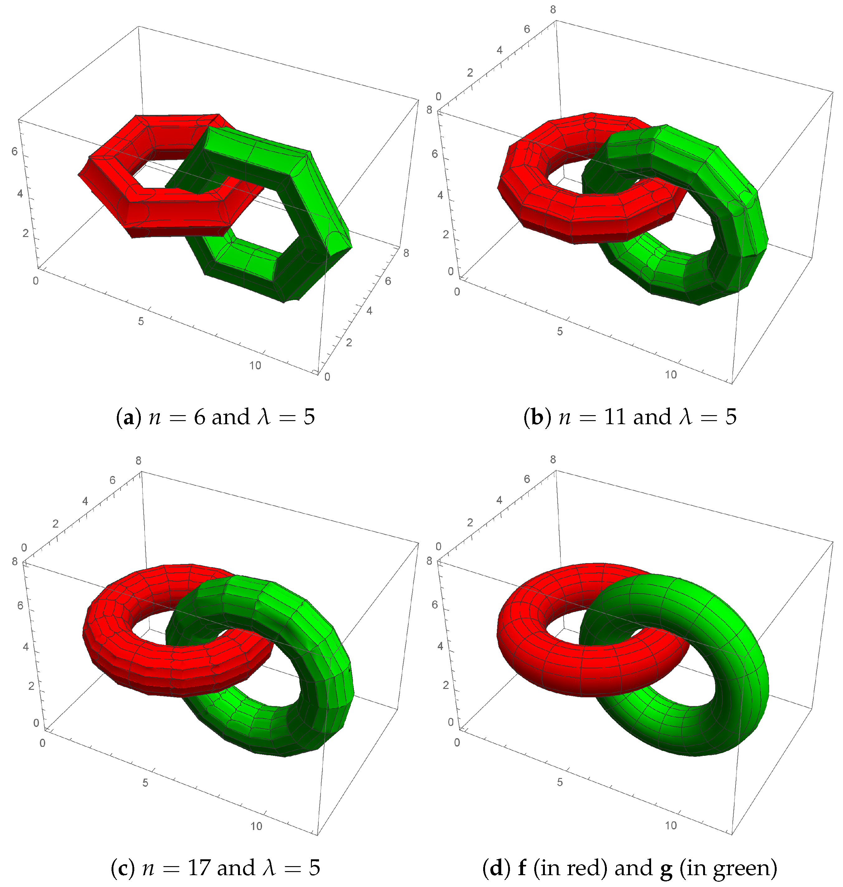
If we consider $\mathbf{f}$ and $\mathbf{g}$ as three-dimensional surfaces parametrized by x and $y,$ we can produce their three-dimensional parametric plots by using the Mathematica program. Similarly, we can also produce the corresponding approximations in (20) and (21) by vector-valued Shepard operators. Such parametric plots are shown in Figure 1 for the values $n=6,11,17$ and $\lambda =5.$

4.2. Approximation Errors in Theorem 1

To numerically support the above application, we now compute the componentwise errors as follows. If $\lambda =5$, examine the corresponding pointwise errors $e_j^{\left[r\right]}$ given by

$$e_j^{\left[r\right]}:=\left|\left({\tilde{\mathbb{S}}}_{n,5}\left(f_r\right)\right)-\left(f_r\right)\right|,r=1,2,3,$$

at the $n_e=30\times 30$ points of a regular mesh of $\mathbf{K}$ for $n=20,50,80$. Here, we consider the function $\mathbf{f}=(f_1,f_2,f_3)$ defined by (18). Observe that, for each $r=1,2,3$, $e_j^{\left[r\right]}$ represents the componentwise approximation errors at the $n_e=30\times 30$ points. In

Table 1. Approximation errors in the first component.

n	${\mathit{e}}_{\mathbf{max}}^{\left[1\right]}$	${\mathit{e}}_{\mathbf{mean}}^{\left[1\right]}$	${\mathit{e}}_{\mathbf{MS}}^{\left[1\right]}$
20	0.35358	0.10099	0.13239
50	0.12529	0.04051	0.04970
80	0.08197	0.02478	0.03056

,

Table 2. Approximation errors in the second component.

n	${\mathit{e}}_{\mathbf{max}}^{\left[2\right]}$	${\mathit{e}}_{\mathbf{mean}}^{\left[2\right]}$	${\mathit{e}}_{\mathbf{MS}}^{\left[2\right]}$
20	0.24870	0.09654	0.11228
50	0.13200	0.03767	0.04773
80	0.08747	0.02391	0.03031

and

Table 3. Approximation errors in the third component.

n	${\mathit{e}}_{\mathbf{max}}^{\left[3\right]}$	${\mathit{e}}_{\mathbf{mean}}^{\left[3\right]}$	${\mathit{e}}_{\mathbf{MS}}^{\left[3\right]}$
20	0.09299	0.03291	0.04278
50	0.03544	0.01313	0.01598
80	0.02172	0.00799	0.00980

, we evaluate the (componentwise) maximum $e_{max}^{\left[r\right]}$, mean $e_{mean}^{\left[r\right]}$ and mean squared $e_{MS}^{\left[r\right]}$ errors defined respectively by

$$e_{max}^{\left[r\right]}:=\underset{1\le j\le n_e}{max}{e}_j^{\left[r\right]},e_{mean}^{\left[r\right]}:=\frac{1}{n_e}\sum _{j=1}^{n_e}{e}_j^{\left[r\right]}\mathrm{and}{e}_{MS}^{\left[r\right]}:=\sqrt{\frac{1}{n_e}\sum _{j=1}^{n_e}{\left(e_j^{\left[r\right]}\right)}^2}$$

for $r=1,2,3$ and $n=20,50,80$ (see [6] for such pointwise errors).

4.3. Effects of Regular Summability Methods

In this subsection, we give some applications of Theorems 3 and 4.

Firstly, in the modification (6), by using the test function ${\mathbf{e}}_0$ in (8), define the vector-valued functions ${\mathbf{u}}_n:\mathbf{K}\to {\mathbb{R}}^d$ by

$${\mathbf{u}}_n\left(\mathbf{x}\right):=\left\{\begin{array}{cc}2{\mathbf{e}}_0\left(\mathbf{x}\right),\hfill & \mathrm{for}n\mathrm{even}\hfill \\ \mathbf{0},\hfill & \mathrm{for}n\mathrm{odd}\hfill \end{array}\right.$$

and also examine the Cesàro method $C_1=\left[c_{jn}\right]$ given by

$$c_{jn}=\left\{\begin{array}{cc}\frac{1}{j},\hfill & \mathrm{if}n=1,2,\dots ,j\hfill \\ 0,\hfill & \mathrm{otherwise}.\hfill \end{array}\right.$$

Consequently, we easily observe that ${\mathbf{u}}_n\stackrel{C_1}{\rightrightarrows }{\mathbf{e}}_0$ on $\mathbf{K}$. Furthermore, for each $\mathbf{f}\in C\left(\mathbf{K},{\mathbb{R}}^d\right)$, if $r=1,2,\dots ,d$, we obtain

$$\begin{array}{cc}\hfill \sum _{n=1}^{\infty }{c}_{jn}{u}_{r,n}{\tilde{\mathbb{S}}}_{n,\lambda }\left(f_r\right)=& \frac{1}{j}\sum _{n=1}^j{u}_{r,n}{\tilde{\mathbb{S}}}_{n,\lambda }\left(f_r\right)\hfill \\ \hfill =& \frac{2}{j}\sum _{n=1}^{[j/2]}{\tilde{\mathbb{S}}}_{2n,\lambda }\left(f_r\right),\hfill \end{array}$$

where $[·]$ denotes the floor function. Then, from the regularity and Theorem 1, the r.h.s. of the last inequality converges to $f_r$ (for each $r=1,2,\dots ,d$) as $j\to \infty$; hence, ${\mathbb{S}}_{n,\lambda }^{\ast }\left(\mathbf{f}\right)\stackrel{C_1}{\rightrightarrows }\mathbf{f}$ on $\mathbf{K}$.

Secondly, in the modification (7) by using the test function ${\mathbf{e}}_1$ in (9), we consider the following function sequences:

$${\mathbf{v}}_n^{\prime }\left(\mathbf{x}\right):=\left\{\begin{array}{cc}2{\mathbf{e}}_1\left(\mathbf{x}\right),\hfill & \mathrm{for}\mathbf{x}\in {[0,\frac{1}{2}]}^m\mathrm{and}n\mathrm{even}\hfill \\ \mathbf{0},\hfill & \mathrm{for}\mathbf{x}\in {[0,\frac{1}{2}]}^m\mathrm{and}n\mathrm{odd}\hfill \\ {\mathbf{e}}_1\left(\mathbf{x}\right),\hfill & \mathrm{otherwise}\hfill \end{array}\right.$$

and

$${\mathbf{v}}_n^{\prime \prime }\left(\mathbf{x}\right):=\left\{\begin{array}{cc}\mathbf{0},\hfill & \mathrm{for}n=k^2\left(k=1,2,\dots \right)\hfill \\ {\mathbf{e}}_1\left(\mathbf{x}\right),\hfill & \mathrm{otherwise}.\hfill \end{array}\right.$$

Using again the Cesàro method, we obtain ${\mathbf{v}}_n^{\prime }\stackrel{C_1}{\rightrightarrows }{\mathbf{e}}_1$ on $\mathbf{K}$ and ${\mathbf{v}}_n^{\prime \prime }\stackrel{\left|C_1\right|}{\rightrightarrows }{\mathbf{e}}_1$ on $\mathbf{K}$. Indeed, for the sequence $\left\{{\mathbf{v}}_n^{\prime }\right\},$ if $\mathbf{x}\notin {[0,\frac{1}{2}]}^m$, it is clear; and also if $\mathbf{x}\in {[0,\frac{1}{2}]}^m$, then

$$\sum _{n=1}^{\infty }{c}_{jn}{\mathbf{v}}_n^{\prime }\left(\mathbf{x}\right)=\frac{\left[j/2\right]2\mathbf{x}}{j}\rightrightarrows {\mathbf{e}}_1\left(\mathbf{x}\right)=\mathbf{x}.$$

On the other hand, for the sequence $\left\{{\mathbf{v}}_n^{\prime \prime }\right\}$, we immediately see that, for every $\mathbf{x}\in \mathbf{K}$,

$$\sum _{n=1}^{\infty }{c}_{jn}\left|v_{r,n}^{\prime \prime }\left(\mathbf{x}\right)-x_r\right|=\frac{1}{j}\sum _{n=1(n=k^2)}^j{x}_r\le \frac{1}{\sqrt{j}}\to 0\mathrm{as}j\to \infty ,$$

which gives ${\mathbf{v}}_n^{\prime \prime }\stackrel{\left|C_1\right|}{\rightrightarrows }{\mathbf{e}}_1$ on $\mathbf{K}$.

Now, in (7), we take the sequences $\left\{{\mathbf{v}}_n^{\prime }\right\}$ and $\left\{{\mathbf{v}}_n^{\prime \prime }\right\}$ instead of $\left\{{\mathbf{v}}_n\right\}$, respectively.

If ${\mathbb{S}}_{n,\lambda }^{\ast \ast }$ is constructed with the sequence $\left\{{\mathbf{v}}_n^{\prime }\right\}$, then we observe that the approximation ${\mathbb{S}}_{n,\lambda }^{\ast \ast }\left(\mathbf{f}\right)$$\stackrel{C_1}{\rightrightarrows }\mathbf{f}$ on $\mathbf{K}$ does not hold for some $\mathbf{f}\in C\left(\mathbf{K},{\mathbb{R}}^d\right)$. For example, considering the function ${\mathbf{e}}_2\left(\mathbf{x}\right)=\left(x_1^2,x_2^2,\dots ,x_d^2\right),$ we obtain, for each $\mathbf{x}\in {[0,\frac{1}{2}]}^m$, that

$$\begin{array}{cc}\hfill \sum _{n=1}^{\infty }{c}_{jn}{\mathbb{S}}_{n,\lambda }^{\ast \ast }({\mathbf{e}}_2;\mathbf{x})=& \frac{1}{j}\sum _{n=1}^j{\mathbb{S}}_{n,\lambda }({\mathbf{e}}_2;{\mathbf{v}}_n\left(\mathbf{x}\right))\hfill \\ \hfill =& \frac{1}{j}\sum _{n=1}^{[j/2]}{\mathbb{S}}_{2n,\lambda }({\mathbf{e}}_2;2\mathbf{x})\hfill \\ \hfill \to & \frac{{\mathbf{e}}_2\left(2\mathbf{x}\right)}{2}\mathrm{as}j\to \infty .\hfill \end{array}$$

Since $\frac{{\mathbf{e}}_2\left(2\mathbf{x}\right)}{2}=\left(2x_1^2,2x_2^2,\dots ,2x_d^2\right)\ne {\mathbf{e}}_2\left(\mathbf{x}\right)$ for $\mathbf{x}\in {[0,\frac{1}{2}]}^m$, one can see that ${\mathbb{S}}_{n,\lambda }^{\ast \ast }({\mathbf{e}}_2;\mathbf{x})\stackrel{C_1}{\nrightarrow }{\mathbf{e}}_2\left(\mathbf{x}\right)$ for each $\mathbf{x}\in {[0,\frac{1}{2}]}^m$.

If ${\mathbb{S}}_{n,\lambda }^{\ast \ast }$ is constructed with the sequence $\left\{{\mathbf{v}}_n^{\prime \prime }\right\}$, then for each $\mathbf{f}\in C\left(\mathbf{K},{\mathbb{R}}^d\right),$ if $\mathbf{x}\in \mathbf{K}$,

$$\begin{array}{cc}\hfill \sum _{n=1}^{\infty }{c}_{jn}\left|{\tilde{\mathbb{S}}}_{n,\lambda }(f_r;{\mathbf{v}}_n^{\prime \prime }\left(\mathbf{x}\right))-f_r\left(\mathbf{x}\right)\right|=& \frac{1}{j}\sum _{n=1(n=k^2)}^j\left|f_r\left(\mathbf{x}\right)\right|+\frac{1}{j}\sum _{n=1(n\ne k^2)}^j\left|{\tilde{\mathbb{S}}}_{n,\lambda }(f_r;\mathbf{x})-f_r\left(\mathbf{x}\right)\right|\hfill \\ \hfill \le & \frac{\left|f_r\left(\mathbf{x}\right)\right|}{\sqrt{j}}+\frac{1}{j}\sum _{n=1}^j\left|{\tilde{\mathbb{S}}}_{n,\lambda }(f_r;\mathbf{x})-f_r\left(\mathbf{x}\right)\right|\hfill \end{array}$$

holds for each $r=1,2,\dots ,d$. Then, from the regularity of $C_1$ and Theorem 1, the r.h.s. of the above inequality uniformly vanishes as $j\to \infty$. Hence, the sequence $\left\{{\mathbb{S}}_{n,\lambda }^{\ast \ast }\left(\mathbf{f}\right)\right\}$ is strongly (uniform) $C_1$-summable to $\mathbf{f}$ on $\mathbf{K}$ for each $\mathbf{f}\in C\left(\mathbf{K},{\mathbb{R}}^d\right)$.

5. Concluding Remarks

In this paper, we established the methodology of approximating continuous vector-valued functions on the unit hypercube using Shepard operators. In order to compute the approximation error, we employed some known error metrics, including maximum error, mean error, and mean squared error. Furthermore, we demonstrated both the theoretical and practical improvements of this approximation by using some techniques from regular summability methods.

In future work, we plan to consider novel vector-valued Shepard processes for approximating functions not necessarily continuous (i.e., integrable functions), the famous Kantorovich operators, interesting in applications for image processing and sampling theory (see [28,29,30]).

References

- Shepard, D. A two-dimensional interpolation function for irregularly-spaced data. In Proceedings of the 23rd ACM National Conference, New York, NY, USA, 27–29 August 1968; ACM: New York, NY, USA, 1968; pp. 517–524. [Google Scholar]
- Barnhill, R.; Dube, R.; Little, F. Properties of Shepard’s surfaces. Rocky Mt. J. Math. 1983, 13, 365–382. [Google Scholar] [CrossRef]
- Barnhill, R.; Ou, H. Surfaces defined on surfaces. Comput. Aided Geom. Des. 1990, 7, 323–336. [Google Scholar] [CrossRef]
- Cavoretto, R.; De Rossi, A.; Dell’Accio, F.; Di Tommaso, F. A 3D efficient procedure for Shepard interpolants on tetrahedra. In Numerical Computations: Theory and Algorithms; Sergeyev, Y.D., Kvasov, D.E., Eds.; Springer International Publishing: Cham, Switzerland, 2020; pp. 27–34. [Google Scholar] [CrossRef]
- Cavoretto, R.; De Rossi, A.; Dell’Accio, F.; Di Tommaso, F. An efficient trivariate algorithm for tetrahedral Shepard interpolation. J. Sci. Comput. 2020, 82, 57. [Google Scholar] [CrossRef]
- Dell’Accio, F.; Di Tommaso, F.; Hormann, K. On the approximation order of triangular Shepard interpolation. IMA J. Numer. Anal. 2016, 36, 359–379. [Google Scholar] [CrossRef]
- Dell’Accio, F.; Di Tommaso, F.; Nouisser, O.; Siar, N. Rational Hermite interpolation on six-tuples and scattered data. Appl. Math. Comput. 2020, 386, 125452. [Google Scholar] [CrossRef]
- Farwig, R. Rate of convergence of Shepard’s global interpolation formula. Math. Comput. 1986, 46, 577–590. [Google Scholar] [CrossRef]
- Criscuolo, G.; Mastroianni, G. Estimates of the Shepard interpolatory procedure. Acta Math. Hung. 1993, 61, 79–91. [Google Scholar] [CrossRef]
- Della Vecchia, B. Direct and converse results by rational operators. Constr. Approx. 1996, 12, 271. [Google Scholar] [CrossRef]
- Della Vecchia, B.; Mastroianni, G. Pointwise simultaneous approximation by rational operators. J. Approx. Theory 1991, 65, 140–150. [Google Scholar] [CrossRef]
- Szabados, J. Direct and converse approximation theorems for the Shepard operator. Approx. Theory Its Appl. 1991, 7, 63–76. [Google Scholar] [CrossRef]
- Yu, D. On weighted approximation by rational operators for functions with singularities. Acta Math. Hung. 2012, 136, 56–75. [Google Scholar] [CrossRef]
- Yu, D.; Zhou, S. Approximation by rational operators in Lp spaces. Math. Nachrichten 2009, 282, 1600–1618. [Google Scholar] [CrossRef]
- Zhou, X. The saturation class of Shepard operators. Acta Math. Hung. 1998, 80, 293–310. [Google Scholar] [CrossRef]
- Duman, O.; Della Vecchia, B. Complex Shepard operators and their summability. Results Math. 2021, 76, 214. [Google Scholar] [CrossRef]
- Duman, O.; Della Vecchia, B. Approximation to integrable functions by modified complex Shepard operators. J. Math. Anal. Appl. 2022, 512, 126161. [Google Scholar] [CrossRef]
- Boos, J.; Cass, P. Classical and Modern Methods in Summability; Oxford Mathematical Monographs, Oxford University Press: Oxford, UK, 2000; p. 600. [Google Scholar]
- Hardy, G.H. Divergent Series; Clarendon Press: Oxford, UK, 1949. [Google Scholar]
- Atlihan, Ö.G.; Orhan, C. Matrix summability and positive linear operators. Positivity 2007, 11, 387–398. [Google Scholar] [CrossRef]
- Atlihan, Ö.G.; Orhan, C. Summation process of positive linear operators. Comput. Math. Appl. 2008, 56, 1188–1195. [Google Scholar] [CrossRef]
- Gökçer, T.Y.; Duman, O. Regular summability methods in the approximation by max-min operators. Fuzzy Sets Syst. 2021, 426, 106–120. [Google Scholar] [CrossRef]
- King, J.P.; Swetits, J.J. Positive linear operators and summability. J. Aust. Math. Soc. 1970, 11, 281–290. [Google Scholar] [CrossRef]
- Mohapatra, R.N. Quantitative results on almost convergence of a sequence of positive linear operators. J. Approx. Theory 1977, 20, 239–250. [Google Scholar] [CrossRef]
- Nishishiraho, T. Convergence rates of summation processes of convolution type operators. J. Nonlinear Convex Anal. 2010, 11, 137–156. [Google Scholar]
- Swetits, J. On summability and positive linear operators. J. Approx. Theory 1979, 25, 186–188. [Google Scholar] [CrossRef]
- Vanderbei, R.J. Uniform Continuity Is Almost Lipschitz Continuity; Statistics and Operations Research Series SOR-91 11; Princeton University: Princeton, NJ, USA, 1991. [Google Scholar]
- Coroianu, L.; Costarelli, D.; Gal, S.G.; Vinti, G. Approximation by multivariate max-product Kantorovich-type operators and learning rates of least-squares regularized regression. Commun. Pure Appl. Anal. 2020, 19, 4213–4225. [Google Scholar] [CrossRef]
- Costarelli, D.; Vinti, G. Approximation by max-product neural network operators of Kantorovich type. Results Math. 2016, 69, 505–519. [Google Scholar] [CrossRef]
- Costarelli, D.; Vinti, G. An inverse result of approximation by sampling Kantorovich series. Proc. Edinb. Math. Soc. 2019, 62, 265–280. [Google Scholar] [CrossRef]
Figure 1.
Parametric plots of (in red) and (in green) for the values and , where and are functions given, respectively, by (18) and (19).