Article

Automatic Sleep Staging Based on Single-Channel EEG Signal Using Null Space Pursuit Decomposition Algorithm

1
School of Science, North China University of Technology, Beijing 100144, China
2
School of Science, China Pharmaceutical University, Nanjing 210009, China
*
Author to whom correspondence should be addressed.
Axioms 2023, 12(1), 30; https://doi.org/10.3390/axioms12010030
Submission received: 27 November 2022 / Revised: 19 December 2022 / Accepted: 20 December 2022 / Published: 27 December 2022

Abstract

:
Sleep quality is related to people’s physical and mental health, so an accurate assessment of sleep quality is key to recognizing sleep disorders and taking effective interventions. To address the shortcomings of traditional manual and automatic staging methods, such as being time-consuming and having low classification accuracy, an automatic sleep staging method based on the null space pursuit (NSP) decomposition algorithm of single-channel electroencephalographic (EEG) signals is proposed, which provides a new way for EEG signal decomposition and automatic identification of sleep stages. First, the single-channel EEG signal data from the Sleep-EDF database, DREAMS Subject database, and Sleep Heart Health Study database (SHHS), available on PhysioNet, were preprocessed, respectively. Second, the preprocessed single-channel EEG signals were decomposed by the NSP algorithm. Third, we extracted nine features in the time domain of the nonlinear dynamics and statistics from the original EEG signal and the six simple signals that were decomposed. Finally, the extreme gradient boosting (XGBOOST) algorithm was used to construct a classification model to classify and identify the 63 extracted EEG signal features for automatic sleep staging. The experimental results showed that, on the Sleep-EDF database, the accuracy of four and five categories were 93.59% and 92.89%, respectively; on the DREAMS Subject database, the accuracy rates of four and five categories were 91.32% and 90.01%, respectively; on the SHHS database, the accuracy rates of four and five categories were 90.25% and 88.37%, respectively. The experimental results show that the automatic sleep staging model proposed in this work has high classification accuracy and efficiency, as well as strong applicability and robustness.

1. Introduction

Sleep is one of the criteria for evaluating the quality of human life and physical health, and we spend one-third of our lives sleeping. Sleep disorders (insomnia, circadian rhythm disturbances, somnolence, and obstructive sleep apnea) are harmful factors that contribute to daytime sleepiness and nighttime insomnia, cognitive and mood disorders, accelerated skin aging, and increased mortality in humans [1]. Therefore, accurate assessment of sleep quality is key to recognizing sleep disorders and implementing effective interventions.
To date, the assessment of sleep quality has been based on the analysis of electroencephalographic (EEG) signals, which are highly stochastic, non-smooth, and nonlinear signals with a frequency range of 0.5 to 50 Hz. The voltage of EEG signals is only about 50 µv. Currently, the first step in the diagnosis of sleep disorders is the staging of the patient’s sleep [2,3], also known as a sleep score. In 2007, the American Academy of Sleep Medicine (AASM) classified the sleep stages as waking (W), non-rapid eye movement (N1, N2, N3), and rapid eye movement (R) [4,5,6,7], where N1, N2, and N3 represent the three stages of non-REM sleep from light to deep sleep, respectively. In order to obtain a polysomnogram (PSG), it is necessary to collect and record relevant signals from the volunteer throughout the sleep time, which include: EEG, electrocardiogram (ECG), electrooculogram (EOG), electromyogram (EMG), respiratory signals, etc. Under the AASM rules, sleep stage labeling (W, N1, N2, N3, R) is performed by sleep specialists every 30 s of the data [8,9,10]. In addition, the traditional manual sleep scoring operation is complex and time-consuming, and the reliability among raters is also a well-known problem. The EEG signals of Stages N1 and W are very similar, as well as Stages R and N3, especially under pathological sleep conditions. Relevant research shows that the average number of errors in scoring by sleep specialists is 13 epochs/PSG [1,9,10].
In order to solve the above problems, many researchers have devoted themselves to developing automatic sleep scoring models in recent years. In 2014, Zhu et al. used features such as the graphic domain of EEG signals to perform 4- and 5-class sleep staging of EEG on the Sleep-EDF database [11], with an accuracy of 89.3% and 88.9%, respectively. In 2017, Hassan et al. used the wavelet transform to decompose the EEG into multiple sub-bands [12], extracted four statistical features of the sub-bands, and used a bootstrap aggregation model (bagging) to classify the EEG in the Sleep-EDF database and the Dreams Subjects database for Class 4 and Class 5 sleep staging, with accuracies of 94.36% and 93.69% and 83.78% and 78.95%, respectively. In 2020, Liu et al. used the ensemble empirical model algorithm (EEMD) to decompose the EEG and extract features of the time domain, statistics, and nonlinear dynamics [13] and used the gradient boosting algorithm to classify the Sleep-EDF database, DREAMS Subjects database, and Sleep Heart Health Study (SHHS) database for 4 and 5 categories of sleep staging of the EEG with accuracies of 93.1% and 91.9%, 86.4% and 83.4%, and 87.5% and 85.8%, respectively.
In 2010, S. L. Peng and W. L. Hwang proposed an adaptive signal decomposition method based on null space pursuit (NSP) [14], which can decompose a nonlinear, non-smooth signal into the sum of a number of simple signals and a residual term, where the simple signals belong to the null space of a second-order differential operator, which makes each simple signal have some physical significance.
In this work, the preprocessed EEG signals from the Sleep-EDF database, DREAMS Subjects database, and SHHS database were firstly decomposed by the NSP algorithm. Secondly, 63 features of the statistics, time domain, and nonlinear dynamics were extracted from the original EEG and, then, decomposed into six simple signals. Finally, an extreme gradient boosting (XGBOOST) algorithm was used to construct the classification model. The experimental results showed that, on the Sleep-EDF database, the accuracy of four and five categories were 93.59% and 92.89%, respectively; on the DREAMS Subject database, the accuracy rates of four and five categories were 91.32% and 90.01%, respectively; on the SHHS database, the accuracy rates of four and five categories were 90.25% and 88.37%, respectively. The automatic sleep staging model proposed in this work not only solves the problems of the time-consuming and subjective factors of manual sleep staging, but also has strong robustness and better classification accuracy, so it has a good application prospect. The workflow of this paper is shown in Figure 1. The main contributions of this paper are as follows:
(1)
An automatic sleep scoring method based on single-channel EEG is proposed.
(2)
A new signal processing technique, NSP decomposition, is used for sleep staging.
(3)
The effectiveness of this method is verified by statistical analysis and graphical analysis.
(4)
Compared with the existing schemes, the performance of this scheme is promising.
(5)
The automation of the classification method avoids the manual time-consuming nature and subjectivity of scoring.

2. Materials and Methods

2.1. Datasets and Data Preprocessing

In this study, the data came from the public data platform PhysioNet and GitHub [15,16,17]. The study protocol of the used datasets was approved by the institutional review board of each participating center, and each participant signed an informed consent form. All methods were carried out in accordance with relevant guidelines and regulations. The current study only analyzed de-identified data from those databases and did not involve a research protocol requiring approval by the relevant institutional review board or ethics committee.
In this work, in order to study the model of automatic sleep staging, we need a large number of EEG signals with known sleep stages. The Sleep-EDF and DREAMS databases are totally free and open. Based on these two open databases, many researchers have made many good research achievements and contributions, which can be used to compare with the results in this work. The SHHS database is not open to the public, but it has great clinical medical value. However, other EEG databases either do have the sleep stage tag, but are not open to the public or do not have the sleep stage tag. The Sleep-EDF database was collected from four male and four female healthy subjects, aged 21–35 years, without any medication and recorded horizontal eye movements, Fpz-Cz leads, and Pz-Oz leads of scalp EEG signals at a sampling frequency of 100 Hz. The sleep classification accuracy of the Pz-Oz lead EEG signal is higher than that of the other leads in the Sleep-EDF database for automatic sleep staging experiments [12,13]. Therefore, we used the Pz-Oz lead EEG signal in the Sleep-EDF database. The DREAMS Subjects database was provided by the sleep laboratory of the Andr Vsale Hospital in Belgium, which recruited healthy adults without any medication, 4 males and 16 females, aged 21 to 48 years, with a sampling frequency of 200 Hz and recorded EEG signals from three leads, Cz-A1, Fp1-A1, and O1-A1. In this work, we used the EEG signal of lead Cz-A1, which has been the most frequently used in previous studies of sleep staging [12,13,18,19]. The SHHS database was collected from 5793 healthy subjects, aged 45 to 70 years, with a sampling frequency of 125 Hz, and the EEG signals of leads C4-A1 and C3-A2 were collected. The EEG signal from the C4-A1 leads were visually “clearer” (lower waveform frequency for the same period of time) than those from the C3-A2 leads [20,21]. Therefore, this paper analyzed the C4-A1 channel EEG signals of 111 subjects (20 males and 91 females) from the SHHS database. Table 1 provides a more intuitive description of the characteristics associated with the three databases.
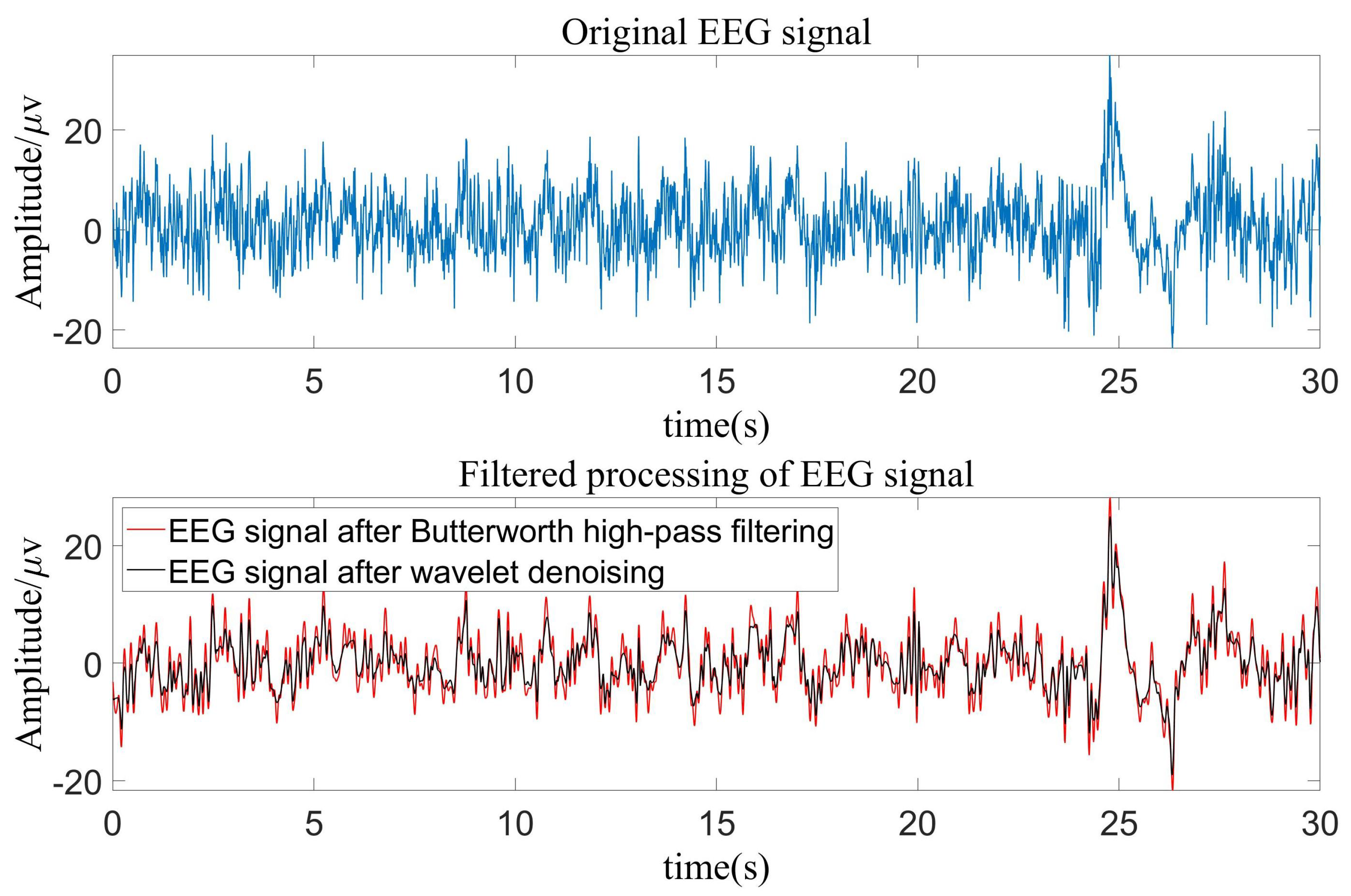
In our research databases, experts gave sleep labels to the EEG signals every 30 s [3]. Therefore, we filtered the original EEG signal every 30 s with a 4th-order Butterworth band-pass filter, which allows only the 0.5 to 50 Hz signal components to pass through. Since wavelet analysis has better denoising performance in the time–frequency domain, the Butterworth band-pass filtered signal was denoised by the wavelet transform in this work. The experiments showed that the results were better when using a db4 wavelet basis and a decomposition layer of 6 [22,23]. Figure 2 shows the results of preprocessing the original 30 s EEG signal.

2.2. Methods

2.2.1. NSP Algorithms

NSP is a fully data-driven adaptive signal decomposition method proposed by S. L. Peng and W. L. Hwang in 2010 [14], which does not require a priori judgment on data features. The algorithm can decompose the input signal S into some simple signals and a residual signal, as shown in Equation (1):
S = j = 1 N U j + R
where R is the residual signal, U j is the simple signal decomposed and satisfying T s ( U j ) = 0 , and α ( t ) is the quadratic of the instantaneous frequency, where T s ( f ( t ) ) = d 2 f ( t ) d t 2 + α ( t ) f ( t ) .
The decomposed signal is obtained by optimizing Equation (2).
min α ( t ) , R , λ 1 , γ , λ 2 T s S R 2 + λ 1 R 2 + γ S R 2 + λ 2 D α ( t ) 2
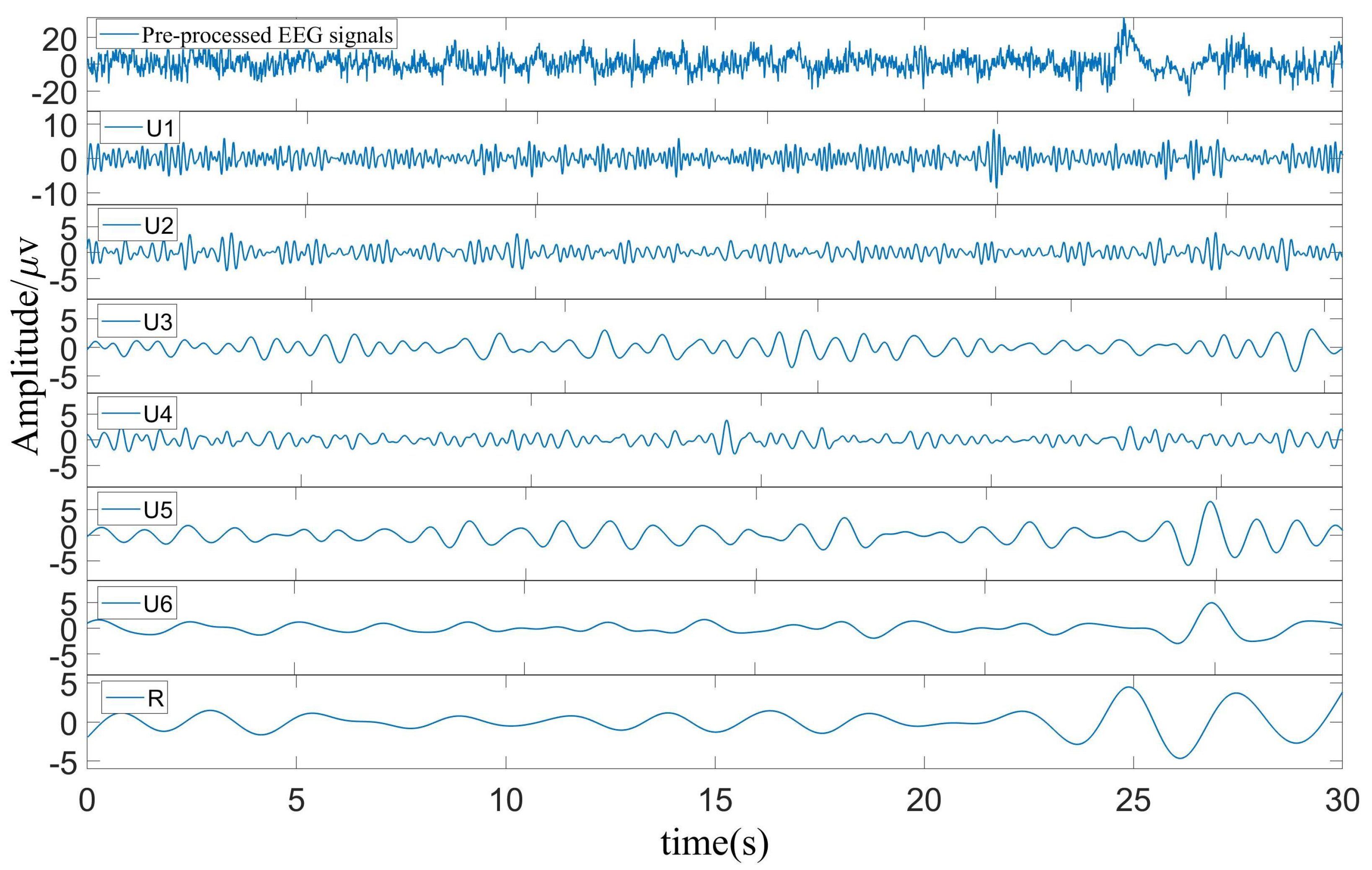
where λ 1 and γ are estimated adaptively by the NSP algorithm, the size of γ determines the total amount of U j residuals in the null space of the operator U j , λ 2 is a constant, and D is a second-order difference operator. Figure 3 shows the results of the decomposition of the preprocessed 30 s EEG signal from the deep sleep stage of one subject in the Sleep-EDF database using the NSP algorithm.

2.2.2. Feature Extraction

In this work, we extracted features from the original EEG signals and the six simple signals decomposed by the NSP algorithm, respectively. The features included: mean (ME), skewness (SK), kurtosis (KU), zero-crossing rate (ZCR), permutation entropy (PE), sample entropy (SE), flexibility (HA), complexity (HC), and mobility (HM). Set S(n) (n = 1, 2, 3, …, M) as a time series, and the mathematical definitions of the above 9 characteristics are given in Table 2.
B m ( r ) and A m + 1 ( r ) are defined as the number of vector pairs in the m- and m + 1 -dimensional reconstruction vectors, whose distances do not exceed the predetermined parameter r, respectively. In this work r was set to 0.15-times the standard deviation, and m was set to 2. In this work r, P was set to 4, so that the full permutation of P is 24, which means L = 24. S ( n ) denotes the difference of S ( n + 1 ) ( n = 1 , 2 , M 1 ) , and S ( n ) ( n = 1 , 2 , M 1 ) . S ¯ is the mean of S ( n ) . ME is the average of S ( n ) . Similarly, S ( n ) is the difference of S ( n + 1 ) and S ( n ) , and S ¯ is the average of S ( n ) . HA is actually the variance of the input signal. HM represents the dominant frequency. HC is the signal bandwidth. Thus, the Hjorth parameter reflects both the time and the frequency domain characteristics of the input signal S ( n ) [28,29]. φ r < 0 is the indicator function.
φ r < 0 ( s ) = 1 , s < 0 , 0 , s 0 .

2.2.3. Classification Algorithms

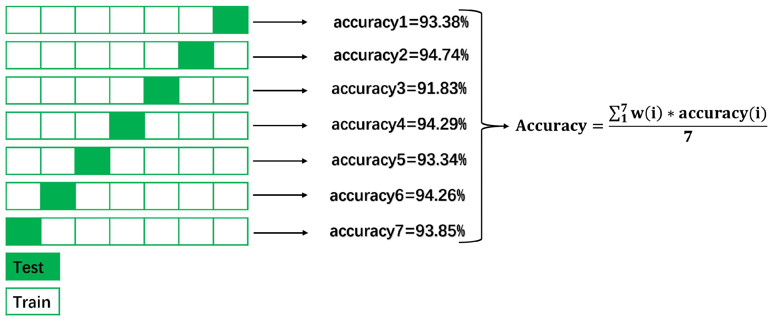
In this work, the sleep stages were divided into 5 categories (W, N1, N2, N3, R) and 4 categories (N1 and N2 were combined into LS). We extracted nine features from the original EEG signals and six simple signals decomposed by the NSP algorithm, respectively. We combined these features into a vector with a dimension of 63 and imported these feature vectors into the XGBOOST classification model for seven-fold cross-validation training and testing. In this work, we divided the dataset into seven parts. One part was used as the verification set or test for each rotation, and the other six parts were used as the training set. The model performance was finally obtained through the weighted average of seven models. The weight of each model depends on the scoring probability.
In 2016, Chen Tianqi et al. proposed the XGBOOST integrated learning algorithm [30], which is an improvement of the gradient boosting tree algorithm (GBDT) [31], which combines several models with lower accuracy into a single high-precision tree model. XGBOOST improves the solution of the loss function in GBDT by performing a second-order Taylor expansion of the loss function and finding the optimal solution after adding a regular term to the loss function. The algorithm has been widely used by data scientists in recent years and has yielded good results in data mining and other areas.

2.2.4. Model Evaluation

The performance of the XGBOOST classifier can be evaluated by calculating the accuracy, specificity, and sensitivity of the classification. The accuracy is the ratio of the sum of the main diagonal elements of the confusion matrix (Q) to the total number of samples (SUM). See Table 3 for the mathematical definitions.
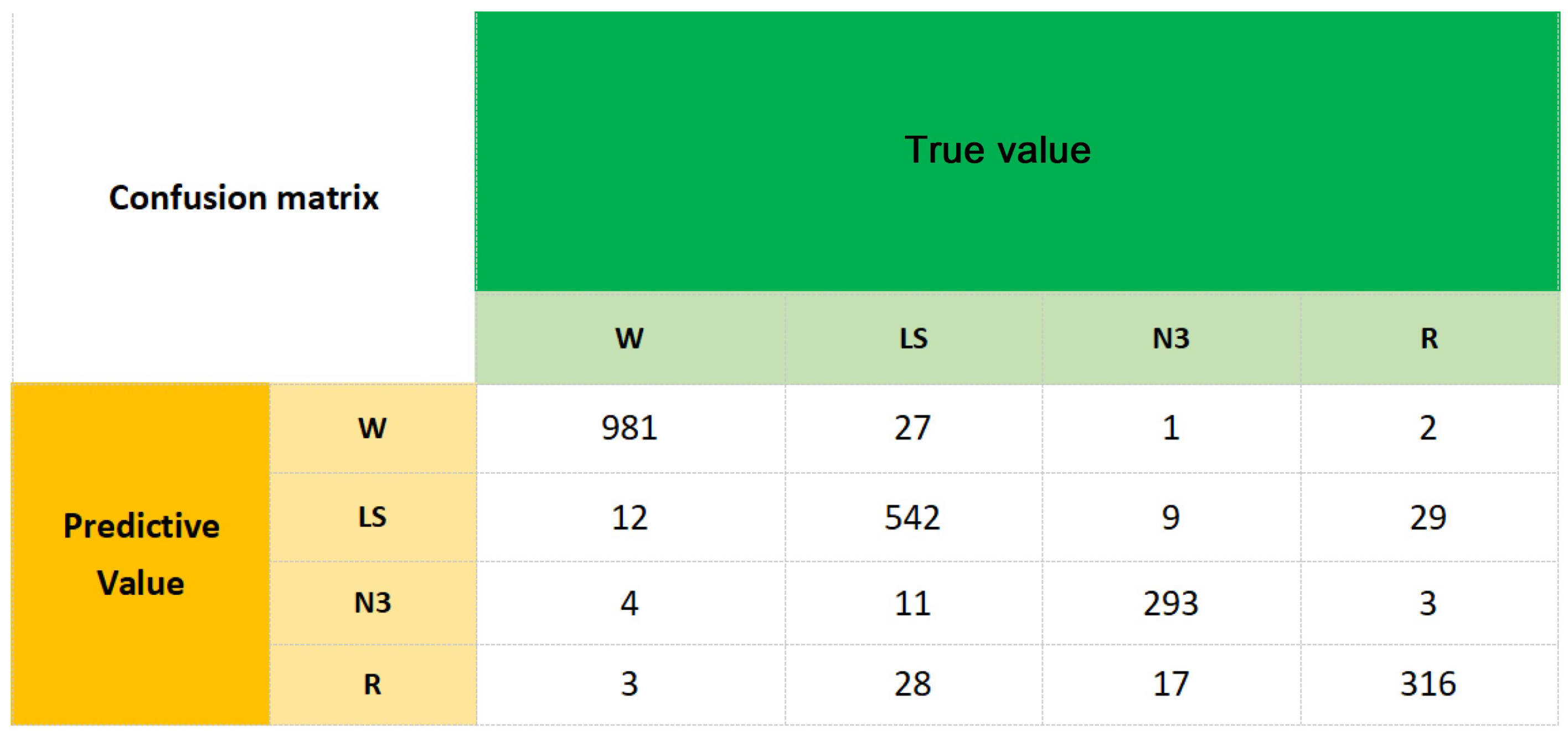
In this work, A = 4 for 4 classification and A = 5 for 5 classification. Figure 4 shows the confusion matrix of Sleep-EDF database 4 classification, in which the data were derived from the average precision of the self-cross-validation model in Figure 5. The diagonal value of the confusion matrix represents the correct number of predictions made by the classifier for this category. The vertical axis of each column represents the actual number of samples for that category. For example, starting from the first column, the number of samples in phase W is 1000. Therefore, the total number of samples (SUM) is the sum of the four columns of the confusion matrix, SUM = 2278.
From the first row of the confusion matrix, we know that the classification model will predict a total of 1011 samples as the W period, of which 981 samples are correctly predicted, while 30 samples are incorrectly predicted.
True positive (TP) means that the real category of the sample is positive and the classification model predicts it as positive. False negative (FN) means that the real category of the sample is positive and the classification model predicts it as negative. False positive (FP) means that the real category of the sample is negative and the model predicts it as positive. True negative (TN) means that the real category of the sample is negative and the classification model predicts it as negative. Therefore, for Stage W, TP = 981, FP = 30, FN = 19. TN = SUM − (TP + FN + FP), TN = 1248 for Stage W. According to the mathematical formula in Table 3, we obtained overall accuracy = 93.59%, specificity = 97.65%, and sensitivity = 98.1% for Phase W. In this work, the specificity and sensitivity calculation results of each category of 4 and 5 sleep stages are shown in Table 4 and Table 5.

3. Results

3.1. Analysis of Classification Results

In order to improve the classification accuracy of the model and prevent overfitting, it is necessary not only to preprocess the training data efficiently, but also to debug many model parameters (gamma, tree depth, learning rate, number of leaves, column sample rate, subsample rate, training times). In this work, the accuracy of the five- and four-class sleep stage classifications of the EEG signals for the three databases are shown in Table 6.
It can be seen from the data in Table 6 that the 4-class classifier model had better classification accuracy than the 5-class classifier model. The accuracy rates of the four classifications corresponding to the three databases were 93.59%, 91.32%, and 90.25%, respectively. Landis and Koch [32] concluded that classifiers with a kappa number greater than 0.80 have near-perfect classification accuracy. Relevant definitions of kappa can be found in [32]. Table 4 shows that our kappa values were greater than 0.8.
According to Table 4, the four classification model had strong sensitivity and specificity for each stage. Table 6 shows that the five-class classifier model had the lowest sensitivity for the N1 sleep stage. There are two reasons for the five-class classifier model having the lowest sensitivity for the N1 sleep stage. First, the proportion of the N1 stage in the three databases is too small: as we can see in Table 6, the proportion of N1 is less than 4% in all three databases, which means there are fewer data for training the model. Second, the similarity of the EEG signal between Stages W and N1 is high. This causes N1 to be easily misidentified. However, the overall performance for other sleep stages was greater than 80%. Therefore, the experimental results further verify the universal applicability and robustness of this classification model.

3.2. Feature Importance Analysis Results

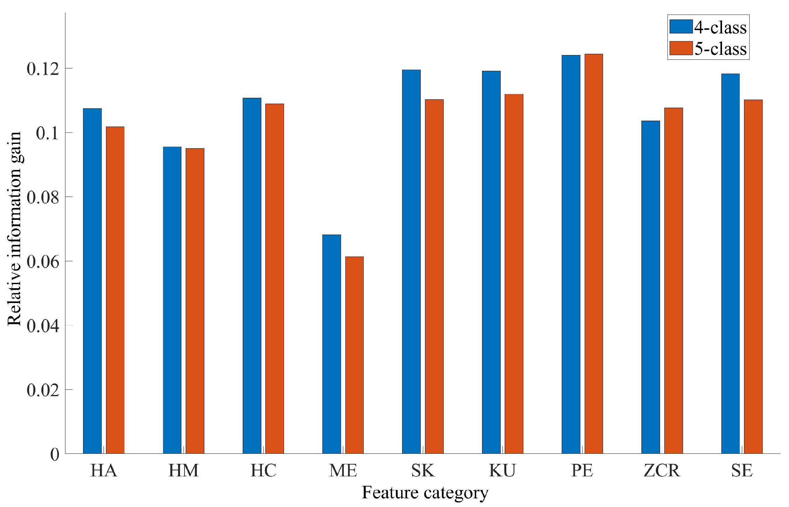
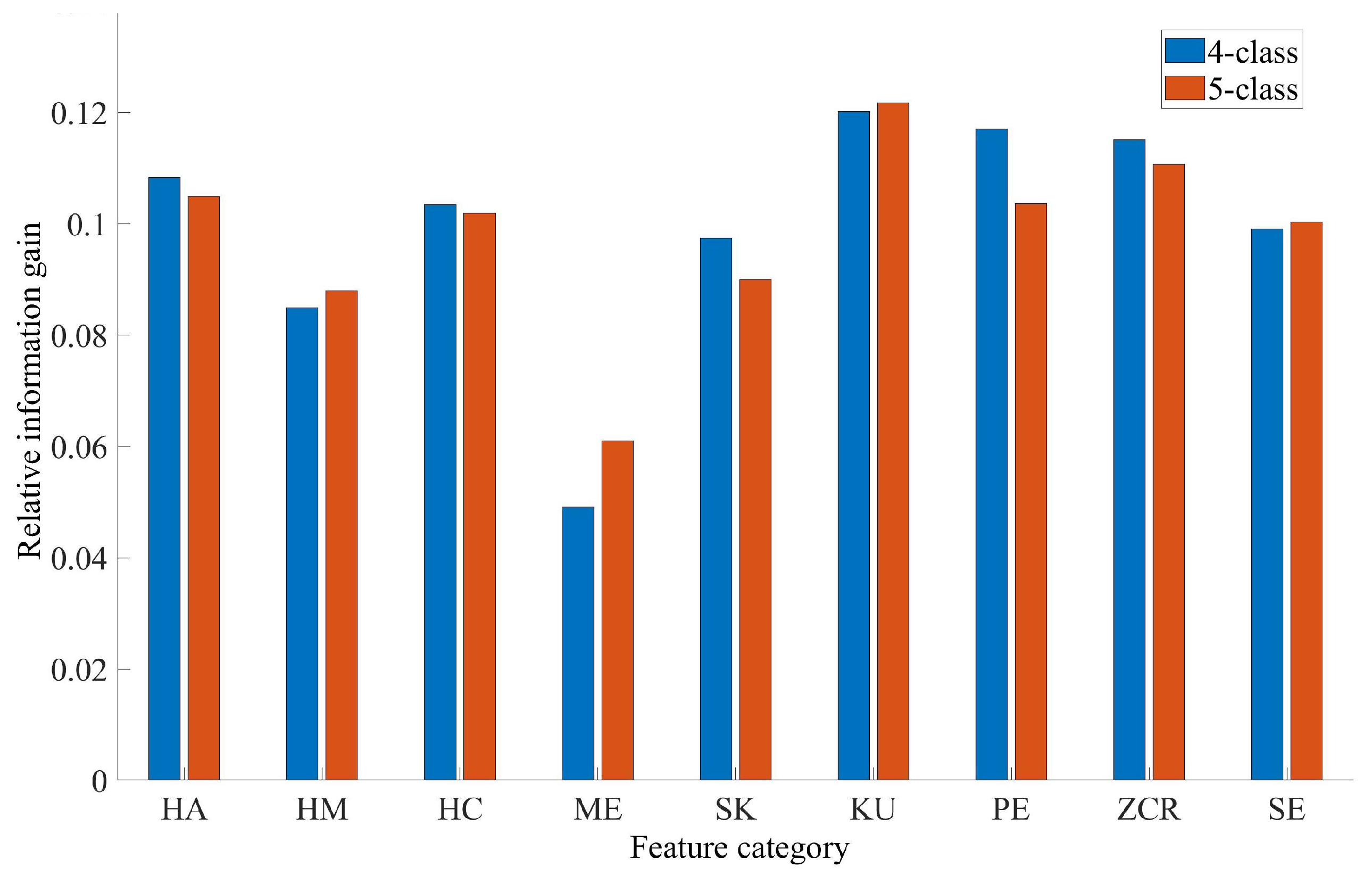
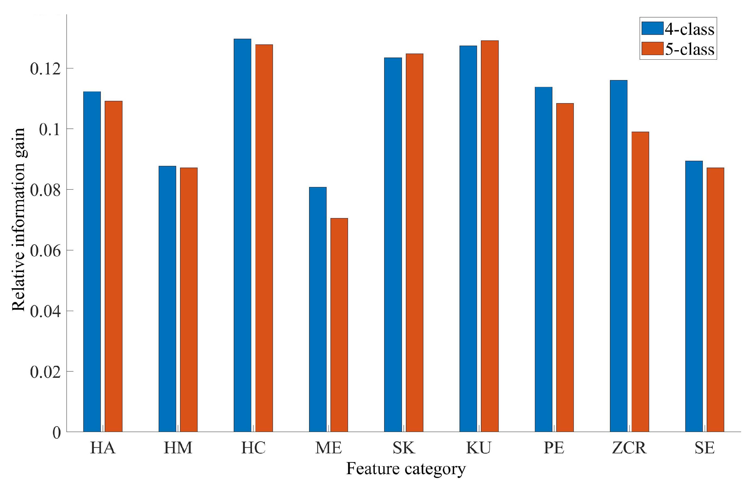
Features are crucial for the classification of sleep stages. Therefore, the importance of features needs to be calculated and evaluated [33]. An information gain graph is the best choice for evaluating the importance of features, which is measured as the proportion relative to the total information gain; the larger the proportion, the more important the feature’s role is in the classification model. The relative information gain of EEG signal features (HA, HM, HC, ZCR, SK, KU, SE, PE) from the Sleep-EDF database, DREAMS Subjects database, and SHHS database was calculated, as shown in Figure 6, Figure 7 and Figure 8. In addition, we also analyzed the characteristic distribution of each sleep stage in the three databases. See the Supplementary Information for details.
As we can see from Figure 6, Figure 7 and Figure 8, the features (HA, HC, SK, KU, PE, SE) have a high relative information gain in the Sleep-EDF database, so they are more active in the classification model. The features (HA, HC, SK, KU, PE, ZCR) are more active in the classification model in the DREAMS Subjects database, while the feature ZCR has the lowest relative information gain and poor adaptability. The features (HA, HC, SK, KU, PE, ZCR) are more active in the classification model of the SHHS database. The above analysis shows that the most active features in the three databases are (HA, HC, SK, KU, PE), followed by the features (ZCR, SE).

4. Discussion

We can see from Table 7 that, in 2017, Hassan proposed a computer-aided sleep stage scoring method using single-channel EEG signals. The tunable-Q wavelet transform (TQWT) was used to decompose EEG signal segments into sub-bands. Then, four statistical moments were extracted from the TQWT sub-bands. Finally, bagging was used for classification. On the Sleep-EDF database, the accuracy rates of 4 categories and 5 categories were 94.36% and 93.69%, respectively, in the study of Hassan. The accuracy was a little higher than ours. However, on the DREAMS Subject database, when the amount of data increased, our average accuracy was 9.3% higher than that study.
We found that most researchers in Table 7 did not preprocess the EEG signals. In this work, we used the fourth-order Butterworth band-pass filter and wavelet de-noising technology. Noise removal using a wavelet has the characteristic of preserving the signal uniqueness even if the noise is minimized [34,35].
Compared with the other two databases, the accuracy was the lowest for the DREAMS Subjects database, as we can see in Table 7. Figure 6, Figure 7 and Figure 8 show that the HA, HC, SA, KU, PE, and ZCR were highly correlated with the sleep stages. However, we can see that the relative information gain of the features was different for the three databases. In this work, we explored a new combination of nine features for classification, which greatly improved the performance of the classification model. We can see from Table 7 that the accuracy of most methods did not increase significantly with the increase of the data. Some methods even obtained decreased accuracy with the increase of the data. In the work of Cong Liu, the accuracy varied greatly with different databases. However, the accuracy of our method for the three different databases was about 90%. This further illustrates the stability and applicability of our method.
We show the research results in recent years in Table 7. Through comparative analysis, it was concluded that decomposition and feature extraction are very important to obtain accurate sleep staging. In this work, we used a completely data-driven approach, the NSP algorithm, to decompose the nonlinear and non-smooth EEG signals. We can see from Table 8 that, if we only analyze the original EEG signals without analyzing the decomposed simple signals, the overall scoring accuracy will be reduced by about 5%. Therefore, NSP decomposition is an effective way to improve the staging accuracy.

5. Conclusions

In this work, an automatic sleep scoring method was proposed. First, NSP was used to decompose the sleep EEG signal fragments, and the characteristics were extracted in the aspects of the time domain, frequency domain, and nonlinear dynamics. The XGBOOST algorithm was used for the classification. Our experimental results showed that this method can accurately detect different sleep states. In addition, compared with the existing sleep scoring system, the performance of the algorithm for our sleep scoring system is satisfactory. In the future, we will focus on the hardware implementation of the algorithm. The feature extraction based on machine learning and various classification models may be an interesting area for further research. Deep learning can also be used to further improve the classification performance.
In this work, the experiments were performed on an Intel(R) Core(TM) i7-8650U CPU @ 1.90GHz 2.11 GHz CPU 16GB computer device. We used Matlab and pytorch for data processing. We calculated the time consumption for the decomposition and classification of a 30-second EEG signal. The NSP algorithm took about 0.101 s to decompose. It took about 0.1 s to classify the sleep stage. Therefore, the high computational efficiency and the high stability of the sleep staging bring a good prospect for the development of wearable devices.

Supplementary Materials

The supporting information can be downloaded at: https://www.mdpi.com/article/10.3390/axioms12010030/s1.

Author Contributions

R.L.: methodology, software, data curation, writing—original draft. W.X.: methodology, software, validation, writing—review, supervision, funding acquisition. H.L. and F.H.: writing—review, supervision. All authors have read and agreed to the published version of the manuscript.

Funding

This research is supported by the Yujie Talent Project of North China University of Technology (Grant No. 107051360022XN735).

Institutional Review Board Statement

Not applicable.

Informed Consent Statement

Not applicable.

Data Availability Statement

The original data supporting the results of this study can be obtained from Sleep-EDF, DREAMS Subject, and SHHS, respectively; however the availability of the original data is limited, and these data were used under the license of the current study, so they cannot be disclosed. However, the original data can be obtained by applying for permission from the database according to the reasonable requirements of the authors and readers. The Supplementary Data provided have been de-identified from the original data.

Acknowledgments

The authors would like to thank the referees and the editor for their useful suggestions, which helped us improve the paper.

Conflicts of Interest

The authors declare no conflict of interest.

References

  1. Younes, M. The case for using digital EEG analysis in clinical sleep medicine. Sleep Sci. Pract. 2017, 1. [Google Scholar] [CrossRef] [Green Version]
  2. Zhao, D.; Wang, Y.; Wang, Q.; Wang, X. Comparative analysis of different characteristics of automatic sleep stages. Comput. Methods Programs Biomed. 2019, 175, 53–72. [Google Scholar] [CrossRef] [PubMed]
  3. Wang, Y.; Loparo, K.A.; Kelly, M.R.; Kaplan, R.F. Evaluation of an automated single-channel sleep staging algorithm. Nat. Sci. Sleep 2015, 7, 101–111. [Google Scholar] [PubMed] [Green Version]
  4. Wolpert, E.A. A manual of standardized terminology, Techniques and scoring system for sleep stages of human subjects. Arch. Gen. Psychiatry. 1969, 20, 246–247. [Google Scholar] [CrossRef]
  5. Kantelhardt, J.W.; Ashkenazy, Y.; Ivanov, P.C.; Bunde, A.; Havlin, S.; Penzel, T.; Peter, J.H.; Stanley, H.E. Characterization of sleep stages by correlations in the magnitude and sign of heartbeat increments. Phys. Rev. E 2002, 65, 051908. [Google Scholar] [CrossRef] [Green Version]
  6. Ferri, R.; Rundo, F.; Novelli, L.; Terzano, M.G.; Parrino, L.; Bruni, O. A new quantitative automatic method for the measurement of non-rapid eye movement sleep electroencephalographic amplitude variability. J. Sleep Res. 2012, 21, 212–220. [Google Scholar] [CrossRef] [PubMed]
  7. Singh, J.; Keer, N. Overview of Telemedicine and Sleep Disorders. Sleep Med. Clin. 2020, 15, 341–346. [Google Scholar] [CrossRef]
  8. Alickovic, E.; Subasi, A. Ensemble SVM Method for Automatic Sleep Stage Classification. IEEE Trans. Instrum. Meas. 2018, 67, 1258–1265. [Google Scholar] [CrossRef] [Green Version]
  9. Punjabi, N.M.; Shifa, N.; Dorffner, G.; Patil, S.; Pien, G.; Aurora, R.N. Computer-assisted automated scoring of polysomnograms using the somnolyzer system. Sleep 2015, 38, 1555–1566. [Google Scholar] [CrossRef] [Green Version]
  10. Koley, B.; Dey, D. An ensemble system for automatic sleep stage classification using single channel EEG signal. Comput. Biol. Med. 2012, 42, 1186–1195. [Google Scholar] [CrossRef]
  11. Zhu, G.; Li, Y.; Wen, P. Analysis and Classification of Sleep Stages Based on Difference Visibility Graphs From a Single-Channel EEG Signal. IEEE J. Biomed. Health Inform. 2014, 18, 1813–1821. [Google Scholar] [CrossRef] [PubMed]
  12. Hassan, A.R.; Subasi, A. A decision support system for automated identification of sleep stages from single-channel EEG signals. Knowl.-Based Syst. 2017, 128, 115–124. [Google Scholar] [CrossRef]
  13. Liu, C.; Tan, B.; Fu, M.; Li, J.; Wang, J.; Hou, F.; Yang, A. Automatic sleep staging with a single-channel EEG based on ensemble empirical mode decomposition. Phys. A Stat. Mech. Its Appl. 2021, 567, 125685. [Google Scholar] [CrossRef]
  14. Peng, S.L.; Hwang, W.L. Null Space Pursuit: An Operator-based Approach to Adaptive Signal Separation. IEEE Trans. Signal Process. 2010, 58, 2475–2483. [Google Scholar] [CrossRef]
  15. The Sleep-EDF Database. Available online: https://physionet.org/content/sleep-edfx/1.0.0/ (accessed on 15 October 2021).
  16. The SHHS Database. Available online: https://physionet.org/content/shhpsgdb/1.0.0/ (accessed on 13 November 2021).
  17. The DREAMS Subjects Database. Available online: https://rdrr.io/github/boupetch/rmdf/man/download_dreams_subjects.html (accessed on 11 November 2021).
  18. Hassan, A.R.; Bhuiyan, M.I.H. Automated identification of sleep states from EEG signals by means of ensemble empirical mode decomposition and random under sampling boosting. Comput. Methods Programs Biomed. 2017, 140, 201–210. [Google Scholar] [CrossRef] [PubMed]
  19. Seifpour, S.; Niknazar, H.; Mikaeili, M.; Nasrabadi, A.M. A new automatic sleep staging system based on statistical behavior of local extrema using single channel EEG signal. Expert Syst. Appl. 2018, 104, 277–293. [Google Scholar] [CrossRef]
  20. Quan, S.F.; Howard, B.V.; Iber, C.; Kiley, J.p.; Nieto, F.j.; O’Connor, G.T.; Rapoport, D.M.; Redline, S.; Robbins, J.; Samet, J.M.; et al. The sleep heart health study: Design, rationale and methods. Sleep 1997, 20, 1077–1085. [Google Scholar] [PubMed] [Green Version]
  21. Redline, S.; Sanders, M.H.; Lind, B.K.; Quan, S.F.; Iber, C.; Gottlieb, D.J.; Bonekat, W.H.; Rapoport, D.M.; Smith, P.L.; Kiley, J.P. Methods for obtaining and analyzing unattended polysomnography data for a multicenter study. Sleep 1998, 21, 759–767. [Google Scholar]
  22. Pan, Q.; Zhang, L.; Dai, G.; Zhang, H. Two denoising methods by wavelet transform. IEEE Trans. Signal Process. 1999, 47, 3401–3406. [Google Scholar] [CrossRef] [Green Version]
  23. Grobbelaar, M.; Phadikar, S.; Ghaderpour, E.; Struck, A.F.; Sinha, N.; Ghosh, R.; Ahmed, M.Z.I. A Survey on Denoising Techniques of Electroencephalogram Signals Using Wavelet Transform. Signals 2022, 3, 577–586. [Google Scholar] [CrossRef]
  24. Fu, K.; Qu, J.; Chai, Y.; Dong, Y. Classification of seizure based on the time frequency image of EEG signals using HHT and SVM. Biomed. Signal Process. Control 2014, 13, 15–22. [Google Scholar] [CrossRef]
  25. Skowronek, J.; Mckinney, M. Features for audio classification: Percussiveness of sounds. Intell. Algorithms Ambient. Biomed. Comput. 2006, 7, 103–118. [Google Scholar]
  26. Richman, J.S.; Moorman, J.R. Physiological time-series analysis using approximate entropy and sample entropy. Am. J. Physiol. Heart Circ. Physiol. 2000, 278, H2039–H2049. [Google Scholar] [CrossRef] [PubMed] [Green Version]
  27. Bandt, C.; Pompe, B. Permutation entropy: A natural complexity measure for time series. Phys. Rev. Lett. 2002, 88, 174102. [Google Scholar] [CrossRef] [PubMed]
  28. Kim, D.J.; Bolbecker, A.R.; Howell, J.; Rass, O.; Sporns, O.; Hetrick, W.P.; Breier, A.; O’Donnell, B.F. Disturbed resting state EEG synchronization in bipolar disorder: A graph-theoretic analysis. Neuroimage Clin. 2013, 2, 414–423. [Google Scholar] [CrossRef] [Green Version]
  29. Cecchin, T.; Ranta, R.; Koessler, L.; Caspary, O.; Vespignani, H.; Maillard, L. Seizure lateralization in scalp EEG using Hjorth parameters. Clin. Neurophysiol. 2010, 121, 290–300. [Google Scholar] [CrossRef]
  30. Chen, T.; Guestrin, C. XGBoost: A scalable tree boosting system. In Proceedings of the 22nd ACM SIGKDD International Conference on Knowledge Discovery and Data Mining, San Francisco, CA, USA, 13–17 August 2016; pp. 785–794. [Google Scholar]
  31. Friedman, J.H. Greedy Function Approximation: A Gradient Boosting Machine. Ann. Stat. 2001, 29, 1189–1232. [Google Scholar] [CrossRef]
  32. Landis, J.R.; Koch, G.G. The Measurement of Observer Agreement for Categorical Data. International Biometric Society. 1977, 33, 159–174. [Google Scholar] [CrossRef] [Green Version]
  33. Koprinska, I. Feature Selection for Brain-Computer Interfaces. In Proceedings of the Pacific-Asia conference on Knowledge of Discovery and Data Mining, New Frontiers in Applied Data Mining, Bangkok, Thailand, 27–30 April 2010; Volume 5669, pp. 106–117. [Google Scholar]
  34. Mamun, M.; Al-Kadi, M.; Marufuzzaman, M. Effectiveness of Wavelet Denoising on Electroencephalogram Signals. J. Appl. Res. Technol. 2013, 11, 156–160. [Google Scholar] [CrossRef] [Green Version]
  35. Phadikar, S.; Sinha, N.; Ghosh, R.; Ghaderpour, E. Automatic Muscle Artifacts Identification and Removal from Single-Channel EEG Using Wavelet Transform with Meta-Heuristically Optimized Non-Local Means Filter. Sensors 2022, 22, 2948. [Google Scholar] [CrossRef]
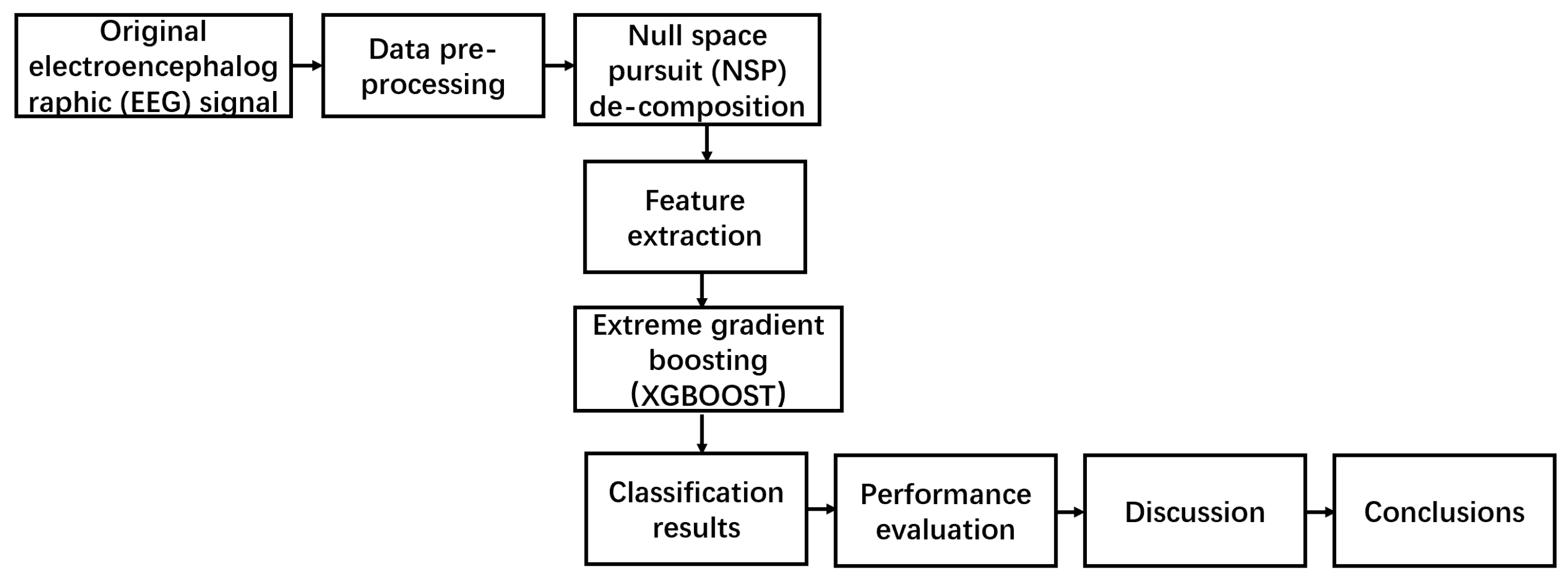
Figure 1. Workflow diagram for model building in this work.
Axioms 12 00030 g001
Figure 2. Original EEG signals and filtered processed EEG signals.
Axioms 12 00030 g002
Figure 3. Decomposition of NSP after preprocessing of the 30-second EEG signal in the deep sleep stage.
Axioms 12 00030 g003
Figure 4. Confusion matrix of Sleep-EDF database 4 classification.
Axioms 12 00030 g004
Figure 5. The 7-fold cross-validation flow chart of Sleep-EDF database 4 classification.
Axioms 12 00030 g005
Figure 6. Relative information gain of Sleep-EDF database features in the XGBOOST model.
Axioms 12 00030 g006
Figure 7. Relative information gain of DREAMS Subjects database features in the XGBOOST model.
Axioms 12 00030 g007
Figure 8. Relative information gain of SHHS database features in the XGBOOST model.
Axioms 12 00030 g008
Table 1. Data characteristics (M is for male, and F is for female).
DatabaseDemographicsElectroencephalographic(EEG)
SubjectsAgeGenderLeadFrequencyEpochs
Sleep-EDF8 28.5 ± 5.4 4M/4FPz-Oz10015188
DREAMS20 33.5 ± 14.6 4M/16FCz-A120020242
SHHS 1 111 57.5 ± 11.3 20M/91FC4-A1125113347
1: SHHS is the abbreviation of Sleep Heart Health Study.
Table 2. Description of the nine features.
FeatureComputing FormulaFeature Description
Mean M E = 1 M n = 1 M S ( n ) ME describes the middle point of the sample set.
Skewness S K = 1 σ 3 n = 1 M S ( n ) M E 3 SK is a measure of the asymmetry of the probability distribution of real variables [24].
Kurtosis K U = 1 σ 4 n = 1 M S ( n ) M E 4 KU is a measure of the kurtosis of the probability distribution of real-valued variables [24].
Zero crossing rate Z C R = 1 M 1 n = 2 M φ r < 0 S ( n ) S ( n 1 ) ZCR is the change rate of the signal sampling point symbol [25].
Sample entropy S E ( S , m , r ) = ln A m + 1 ( r ) / B m ( r ) SE is often used to measure the complexity of time series [26].
Permutation entropy P E = t = 1 L ξ t ln ( ξ t ) PE can quickly and accurately respond to the sudden change of the signal,
which is a standard to measure the complexity of the signal [27].
Flexibility H A = σ 2 = 1 M n = 1 M S ( n ) M E 2 HA represents the fluctuation degree of the EEG signal [28].
Complexity H M = n = 1 M 1 S ( n ) S ¯ 2 / ( M 1 ) / n = 1 M S ( n ) M E 2 / ( M 1 ) HM represents the slope of the EEG signal [28].
Mobility H C = n = 1 M 2 S ( n ) S ¯ 2 / ( M 2 ) / n = 1 M 1 S ( n ) S ¯ 2 / ( M 1 ) n = 1 M 1 S ( n ) S ¯ 2 / ( M 1 ) / n = 1 M S ( n ) M E 2 / M HC represents the change rate of the slope of the EEG signal [28,29].
Table 3. Calculation formula for model evaluation.
Model EvaluationComputing Formula
Accuracy a c c u r a c y = i = 1 A Q i i S U M
Specificity s p e c i f i c i t y = T N T N + F P
Sensitivity s e n s i t i v i t y = TP T P + F N
Table 4. The sensitivity and specificity of 4-class classification.
Database 4-Class Classifier
WLSN3R
Sleep-EDFspecificity97.65%97.00%96.08%91.51%
sensitivity98.1%89.14%91.56%95.75%
DREAMSspecificity95.23%93.87%92.15%83.24%
sensitivity96.11%92.87%90.06%80.42%
SHHSspecificity94.06%90.53%88.32%95.84%
sensitivity90.08%93.74%92.51%94.73%
Table 5. The sensitivity, specificity, and proportion of each stage of 5-class classification.
Database 5-Class Classifier
WN1N2N3R
Sleep-EDFspecificity96.41%94.46%93.63%93.11%85.38%
sensitivity98.67%47.36%90.57%90.68%85.60%
proportion53.03%3.1%23.9%8.8%11.17%
DREAMSspecificity93.96%91.47%89.81%87.39%81.53%
sensitivity95.18%59.32%89.85%92.12%83.10%
proportion35%3.4%28.6%13%20%
SHHSspecificity95.84%92.03%91.00%89.69%84.33%
sensitivity94.73%9.21%92.00%89.09%81.90%
proportion27.65%2.6%39.4%14.8%15.55%
Table 6. Classification model accuracy and kappa.
Database 4-Class Classifier5-Class Classifier
Sleep-EDFAccuracy93.59%92.89%
Kappa0.89240.8837
DREAMSAccuracy91.32%90.01%
Kappa0.86190.8392
SHHSAccuracy90.25%88.37%
Kappa0.84120.8238
Table 7. Comparison of experimental results.
DatabaseYearNameDecomposition AlgorithmFeatures ang Signal ChannelClassifiers4-Class5-Class
Sleep-EDF2014Zhu Degree distribution
based on
difference visibility
(Pz-Oz)
Support vector
machine
89.3%88.9%
2017HassanTunable-Q factor
wavelet transform
Four statistical
moments
(Pz-Oz)
Bagging94.36%93.69%
2018Seifpour Statistical behavior of
local extrema
(Fpz-Cz)
Support vector
machine
92.8%91.8%
2021Cong LiuEnsemble empiricar
model algorithm (EEMD)
Mean, skewness, kurtosis,
time domain, and nonlinear dynamics
features
(Pz-Oz)
XGBOOST93.1%91.9%
In this workNSPMean, skewness, kurtosis,
time domain, and nonlinear dynamics
features
(Pz-Oz)
XGBOOST93.59%92.89%
DREAMS Subjects2017HassanEEMDStatistical features
(Cz-A1)
Random under
sampling boosting
80.0%74.6%
2017HassanTunable-Q factor
wavelet transform
Four statistical
moments
(Cz-A1)
Bagging83.78%78.95%
2018Seifpour Statistical behavior of
local extrema
(Cz-A1)
Support vector
machine
83.3%
2021Cong LiuEEMDMean, skewness, kurtosis,
time domain, and nonlinear dynamics
features
(Cz-A1)
XGBOOST86.4%83.4%
In this workNSPMean, skewness, kurtosis,
time domain, and nonlinear dynamics
features
(Cz-A1)
XGBOOST91.32%90.01%
SHHS2021Cong LiuEEMDMean, skewness, kurtosis,
time domain, and nonlinear dynamics
features
(C4-A1)
XGBOOST87.5%85.8%
In this workNSPMean, skewness, kurtosis,
time domain, and nonlinear dynamics
features
(C4-A1)
XGBOOST90.25%88.37%
Table 8. Classification accuracy using or not NSP decomposition.
Database 4-Class Classifier5-Class Classifier
Sleep-EDFAccuracy of using NSP93.59%92.89%
Accuracy without NSP89.56%88.20%
DREAMSAccuracy of using NSP91.32%90.01%
Accuracy without NSP84.34%82.63%
SHHSAccuracy of using NSP90.25%88.37%
Accuracy without NSP85.73%81.58%
Disclaimer/Publisher’s Note: The statements, opinions and data contained in all publications are solely those of the individual author(s) and contributor(s) and not of MDPI and/or the editor(s). MDPI and/or the editor(s) disclaim responsibility for any injury to people or property resulting from any ideas, methods, instructions or products referred to in the content.