Analysis of Finite Solution Spaces of Second-Order ODE with Dirac Delta Periodic Forcing

Abstract

Second-order Ordinary Differential Equations (ODEs) with discontinuous forcing have numerous applications in engineering and computational sciences. The analysis of the solution spaces of non-homogeneous ODEs is difficult due to the complexities in multidimensional systems, with multiple discontinuous variables present in forcing functions. Numerical solutions are often prone to failures in the presence of discontinuities. Algebraic decompositions are employed for analysis in such cases, assuming that regularities exist, operators are present in Banach (solution) spaces, and there is finite measurability. This paper proposes a generalized, finite-dimensional algebraic analysis of the solution spaces of second-order ODEs equipped with periodic Dirac delta forcing. The proposed algebraic analysis establishes the conditions for the convergence of responses within the solution spaces without requiring relative smoothness of the forcing functions. The Lipschitz regularizations and Lebesgue measurability are not considered as preconditions maintaining generality. The analysis shows that smooth and locally finite responses can be admitted in an exponentially stable solution space. The numerical analysis of the solution spaces is computed based on combinatorial changes in coefficients. It exhibits a set of locally uniform responses in the solution spaces. In contrast, the global response profiles show localized as well as oriented instabilities at specific neighborhoods in the solution spaces. Furthermore, the bands of the expansions–contractions of the stable response profiles are observable within the solution spaces depending upon the values of the coefficients and time intervals. The application aspects and distinguishing properties of the proposed approaches are outlined in brief.

1. Introduction

Ordinary differential equations (ODEs) have a wide array of applications with respect to modeling engineering systems and performing numerical (computational) analyses of data. The systems of differential equations often contain discontinuous forcing functions (or forcing factors) with applications in physics, engineering, data science, biology, and geology [1,2,3]. The comprehensive treatments concerning the solving of differential equations with discontinuous and periodic forcing functions stem from Filippov [4]. The generalized form of such equations (termed feedback equations) with single-variable discontinuity can be represented as $\stackrel{•}{x}=Ax-BF(x)$, where $F(x)$ is a discontinuous forcing function and $A,B$ are the constant matrices of finite dimensions [5]. However, if a differential equation contains multi-variable discontinuous forcing, then the corresponding two-variable forcing can be represented as $F_2(x,t)$, which has numerous applications in physical systems modeling [1]. It has been noted that the determination of classical solutions to such an equation is both difficult and insufficient [5,6]. Furthermore, the numerical solution techniques using software solvers are often prone to failures due to the presence of discontinuous forcing functions [7]. In order to simplify the equation for the determination of an analytical solution, it is often assumed that the single-variable discontinuous function $F(x)$ is finitely Lebesgue-measurable and linear. Similar problems arise regarding differential equations in the four-dimensional numerical analysis of meteorological data, which are equipped with the discontinuous forcing function given in the form $G(u(x,t),x,t)$, where $(x,t)$ is a pair of space-time variables and the first variable is a function represented as $u=f(x,t){|}_c$ at a critical state $c$ representing the state of discontinuity [8]. In this particular case, the analytic evaluation of the term $\partial G/\partial u$ is not straightforward; as a consequence, a different functional form is formulated, which is given as $F_2(x,t)=G(u(x,t),x,t)$. However, such a function does not greatly reduce analytical complexity. Thus, the discontinuous forcing function $F_2(x,t)$ is further algebraically decomposed as $F_2(x,t)=S(x)D(t)$, where $S(x)\in C^{\infty }$ and the function $D(t)$ constitutes a discontinuous function [8].

1.1. Motivations

The presence of (discontinuous) Dirac delta functions in the forcing factor is often considered as multiplicative variety. These types of differential equations with Dirac delta discontinuity have numerous applications in non-smooth mechanics [9,10,11,12]. In general, the multiplicative variety of a differential equation with Dirac delta forcing is given as $dy/dt=u(t,y)+v(y)\delta (t)$, where $\delta (t)$ is the Dirac function. In general, the solution is formulated by incorporating regularizations, wherein the continuous function $u(.,.)$ should be locally Lipschitz with respect to $y$ and it should be compact in terms of its time interval within the solution space [12]. Moreover, the additionally required condition is that the function $v(.)$ should have the following property: $v\in C^1(R)$, where $R$ is the set of real numbers. It is known that if $u(.,.)$ and $v(.)$ are globally Lipschitz, then the solution is a convergent (limiting) function [12]. In this case, the restriction is that regularization is mandatory to find a solution if the singularity is superimposed at the initial condition. This motivated us to ask a general question: How do we algebraically analyze a second-order differential equation with periodic Dirac delta forcing given in general form? Moreover, our corollary question is as follows: what are the behaviors of such equations under additive as well as discontinuous and impulsive forcing factors? We address these questions comprehensively in this paper.

1.2. Contributions

The contributions made in this paper can be summarized as follows: We present the generalized algebraic analysis and numerical simulations of the behavior of solution spaces of non-homogeneous ODEs endowed with Dirac delta periodic forcing (refer to Equation (1)). Our algebraic analysis considers the combinatorial changes in the set of coefficients of the ODE. The algebraic analysis of the convergence of solution within an exponentially stable solution space is presented by employing the polynomial expansions of functions. The proposed algebraic analysis of the solution space does not employ any external function decomposition or Lipschitz regularizations as preconditions. It is shown that discontinuous periodic forcing can be regularized within a smooth, exponential solution space admitting locally finite responses. This results in the formation of sharp boundaries of stable responses and occasional appearances of instabilities at specific neighborhoods within the solution spaces, mostly at sharp boundaries. We present the numerical analysis of local and global response profiles in-detail under varying coefficients and time intervals within the solution spaces, while considering different algebraic relations between the constant factors of the governing equation. The results of the numerical analysis are presented as a set of surface maps exposing the interrelationships between the ranges of constant factors, the algebraic relations between them, and the degree of non-linearity covering negative and positive domains. In this paper, DD stands for Dirac Delta, which generates a periodic forcing factor of the non-homogeneous ODE. The sets of real numbers and integers are denoted by $R,Z$ respectively, where $R=(-\infty ,+\infty )$.

The rest of the paper is organized as follows. The algebraic analysis is presented in Section 2. Section 3 presents the numerical simulations in detail. Section 4 presents the application aspects of the proposed analysis. Finally, Section 5 concludes the paper.

2. Analysis of ODE with Periodic DD Forcing

The general form of a second-order non-homogeneous ODE with a periodic DD forcing factor can be represented as given in the following equation (note that $D$ is a differentiation operator and the product $f(t)\delta (t)$ constitutes forcing):

$$\begin{array}{l}{D}^{2}x+k{x}^n={\displaystyle \sum _{t=0}^{t=+\infty }f(t)\delta (t)},\\ k\in R\backslash \left\{0\right\}.\end{array}$$

(1)

Note that the forcing factor is of the discrete (discontinuous) variety, controlling the dynamic behavior of the equation in the solution space. Moreover, it is considered that the sequence generated by the periodic DD forcing factor must be convergent for the solution to exist. Note that in almost all practical application cases, the finite subsequences are considered due to computational limitations (i.e., practical cases consider the presence of convergence within bounded solution spaces). The corresponding finite form of the general equation for the terms $N\in Z^{+}$ can be formulated as:

$$\begin{array}{l}{D}^{2}x+k{x}^n={\displaystyle \sum _{t=0}^{t=N}f(t)\delta (t)},\\ 1\le N<+\infty .\end{array}$$

(2)

Let us consider the corresponding homogeneous equation with an exponentially smooth variety of solutions in the solution spaces for the ODE under investigation. Let $x=a{e}^{bt},\{a,b\}\subset R$ be a solution of a homogenized form of Equation (2). This leads to the following algebraic conditions to be satisfied:

$$\begin{array}{l}a{b}^2+k{a}^n{e}^{(n-1)bt}=0,\\ and,\\ x=-\left(k{a}^n/b^2\right)e^{nbt}.\end{array}$$

(3)

It is important to note that the solution of $x$ given in Equation (3) is applicable only for the homogenized form of Equation (2). However, as Equation (2) is not in a homogeneous form, we need to resolve the degree of discrete forcing by using the corresponding series within the solution spaces. Let us consider that there is a sequence in time ${⟨s_t⟩}_{t=0}^{t=+\infty }$ at a finite interval such that $s_t\in [-{\alpha }_1,+{\alpha }_2]$, where ${\alpha }_i\in R,i\in \{1,2\}$ are the boundaries. As a subsequence of a bounded sequence is convergent following the Cauchy criteria, the periodic DD forcing factor can be represented as:

$$\begin{array}{l}{⟨v_t⟩}_{t=0}^{t=N}\subset {⟨s_t⟩}_{t=0}^{t=+\infty },\\ {\displaystyle \sum _{t=0}^{t=N}f(t)\delta (t)={\displaystyle \sum _{t=0}^{t=N}{v}_t}.}\end{array}$$

(4)

This leads to the following result in view of the algebraic expansion of Equation (3), while considering the preservation of the conditions given in Equation (4):

$$a{b}^2+k{a}^n+(n-1)k{a}^{n}bt+({(n-1)}^2/2!)k{a}^n{(bt)}^2+\dots \dots ={\displaystyle \sum _{t=0}^{t=N}{v}_t}.$$

(5)

In order to resolve the finite series at multiple time instants, we need a set of varying sums of sequences satisfying Equation (5). Let us consider a discrete and convergent sequence space; then, we construct a set of series at different time instants, as given below:

$$\begin{array}{l}[t=0]\Rightarrow [{\epsilon }_t=0],\\ [t=1]\Rightarrow [{\epsilon }_t=(n-1)b+((n-1{)}^2/2)b^2+((n-1{)}^3/3!)b^3+\dots \dots ],\\ [t=2]\Rightarrow [{\epsilon }_t=2(n-1)b+2(n-1{)}^2{b}^2+(4/3)(n-1{)}^3{b}^3+\dots \dots ],\\ \dots \dots \\ [t=N]\Rightarrow [{\epsilon }_t=bN((n-1)+(1/2)(n-1{)}^{2}bN+(1/3!)(n-1{)}^3(bN{)}^2+\dots \dots )].\end{array}$$

(6)

Note that Equation (5) is of a discrete variety, and it needs to satisfy the following algebraic conditions by considering Equation (6):

$$\begin{array}{l}{v}_t=a{b}^2+k{a}^n(1+{\epsilon }_t),\\ {\epsilon }_t<{\epsilon }_{t+1}.\end{array}$$

(7)

This immediately leads to the following set of results, which are presented as a set of theorems that consider the degree of non-linearity ($n$) as a constant, while the other set of constants $\{a,b,k\}$ is considered to constitute finite-valued elements. We present the first result in the following theorem considering Equation (7).

Theorem 1.

If ${⟨{\epsilon }_t⟩}_{t=1}^{+\infty }$ is a Cauchy sequence with  $b>0$ , then  $L_v={\lim }_{t\to +\infty }\left({\displaystyle \sum _t{v}_t}\right)$ is not convergent if  $ka\ne 0$.

Proof. 

Let us consider a Cauchy sequence ${⟨{\epsilon }_t⟩}_{t=1}^{+\infty }$ such that $b>0$. Note that in this case the condition of $\forall t\in (0,+\infty ], {\epsilon }_t>0$ is preserved, and the sequence ${⟨{\epsilon }_t⟩}_{t=1}^{+\infty }$ is not considered to be bounded as a precondition. Thus, if the corresponding sum of the series is computed as $l={\displaystyle \sum _t(1+{\epsilon }_t)}$, then we can conclude that $l\to +\infty$ as $t\to +\infty$. As a consequence, the sum of the limiting value, computed as $L_v={\lim }_{t\to +\infty }\left({\displaystyle \sum _t{v}_t}\right)$, is not convergent if $ka\ne 0$. □

This leads to the following lemma representing the strict boundedness condition of $L_{v(N)}={\lim }_{t\to N}\left({\displaystyle \sum _t{v}_t}\right)$ within the local space of responses.

Lemma 1.

If $b\in [0,1)$ and  $N<+\infty$, then $L_{v(N)}$ is strictly convergent.

Proof. 

If we consider that $b\in [0,1)$, we obtain the condition given as $b^m>b^{m+1}$. As a result, we can conclude that ${\epsilon }_t\in (0,M)$, where $M<+\infty$ and $t\in (0,N]$. Hence, if we consider an exponentially stable and finite solution space with $N<+\infty$, then $-\infty <K_l\le L_{v(N)}\le K_h<+\infty$, depending on the values of the set of constants $\{a,n\}$, and as a result $L_{v(N)}$ is strictly convergent. Note that the finite boundaries $K_l,K_h$ are real numbers. □

On the other hand, if we impose an additional condition on Equation (7) such that $b<0,{\epsilon }_t<0$, we obtain the corresponding convergence criteria presented in the following theorem as a result.

Theorem 2.

If the sequence  ${⟨{\epsilon }_t⟩}_{t=1}^{+\infty }$ maintains the conditions that $b<0, {\epsilon }_t<{\epsilon }_{t+1}<0$ and  ${\epsilon }_t\to -1$ , then  ${\lim }_{t\to +\infty } v_t$ is convergent.

Proof. 

The proof is relatively straightforward. In this case, the sequence ${⟨{\epsilon }_t⟩}_{t=1}^{+\infty }$ is a monotone sequence if we consider that ${\epsilon }_t<{\epsilon }_{t+1}$; moreover, it is possible that ${\epsilon }_t\to -1$ if we impose the following restriction: ${\epsilon }_t\in (-\infty ,-1]$. As a result, the limit $({\lim }_{t\to +\infty }{v}_t)\to a{b}^2$ is convergent, wherein the set of constants $\{a,b\}$ is finite-valued. □

Remark 1.

It is important to note in Theorem 2 that ${\lim }_{t\to +\infty } v_t$ is finite even if  $k\ne 0$ . In other words, in this case, the convergence of  $v_t$ is independent of the vanishing $k$ . Moreover, we can generalize the observation by the condition as $\forall t\in [0,+\infty ], {\epsilon }_t\in R$ indicating that  ${\epsilon }_t$ is finite at every time instant if the sequence  ${⟨{\epsilon }_t⟩}_{t=1}^{+\infty }$ is a finitely bounded Cauchy sequence.

Note that we have mentioned earlier that the complete solution of a non-homogeneous ODE with periodic DD forcing needs to be convergent within the solution spaces. The representation of Equation (7) and the aforesaid theorems illustrate that convergence analysis is necessary within the solution space to maintain the finiteness of the responses of the ODE under periodic DD forcing at different time instants. The detailed algebraic analyses of the sequential convergence of the terms within the solution space are presented in the following subsection.

Convergence Analysis

These algebraic convergence analyses consider the complete solution of a generalized non-homogeneous ODE along with the incorporated periodic DD forcing factor. The following identity must be satisfied by the complete solution space of the non-homogeneous ODE with discontinuities:

$$a{b}^2+k{a}^n{e}^{(n-1)bt}=a{b}^{2}N+k{a}^n{\displaystyle \sum _{t=0}^{t=N}(1+{\epsilon }_t).}$$

(8)

This leads to the following conclusion considering the condition that $k{a}^n\in R\backslash \left\{0\right\}$, where an exponential function is strictly convergent (because the solution space is finite):

$$\begin{array}{l}-\infty <{\displaystyle \sum _{t=0}^{t=N}(1+{\epsilon }_t)<+\infty ,}\\ {\displaystyle \sum _{t=0}^{t=N}(1+{\epsilon }_t)=e^{(n-1)bt}+\left(\frac{1-N}{k{a}^n}\right)a{b}^2.}\end{array}$$

(9)

The above algebraic condition controlling the proposed exponential type of response is of a smooth variety and is convergent, thereby resolving the non-homogeneities generated by the periodic DD forcing factor. The solution space is termed a locally stable space if we consider a finite time interval $[0,N]$, where the responses are also finite. We can derive an interesting observation, as presented in the following theorem, before proceeding to the numerical simulations.

Theorem 3.

If the solution space is locally stable in the finite time interval $[0,N]$, then it preserves the condition $-\infty <{\epsilon }_t<+\infty$ and  $ka\ne 0$.

Proof. 

Let us consider Equation (9) such that ${\displaystyle \sum _{t=0}^{t=N}(1+{\epsilon }_t)-e^{(n-1)bt}=a^{(1-n)}{k}^{-1}{b}^2(1-N)}$. Note that the right side of the expression is a constant and finite if $ka\ne 0$. Hence, the expression ${\displaystyle \sum _{t=0}^{t=N}(1+{\epsilon }_t)-e^{(n-1)bt}}$ is convergent at the time interval $[0,N]$, indicating that $-\infty <{\epsilon }_t<+\infty$ at the local responses within the locally stable solution space. □

It can be observed from Theorem 3 that the finiteness of ${\epsilon }_t$ can be admitted under the convergence conditions. The local and global behaviors of the response profiles of the ODE within the solution space are numerically analyzed in-detail in the following section.

3. Numerical Analysis

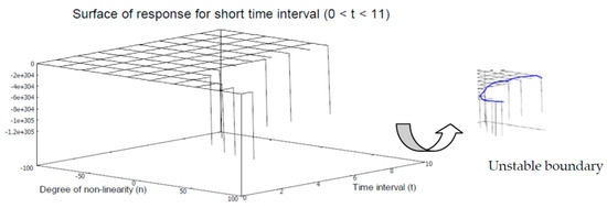
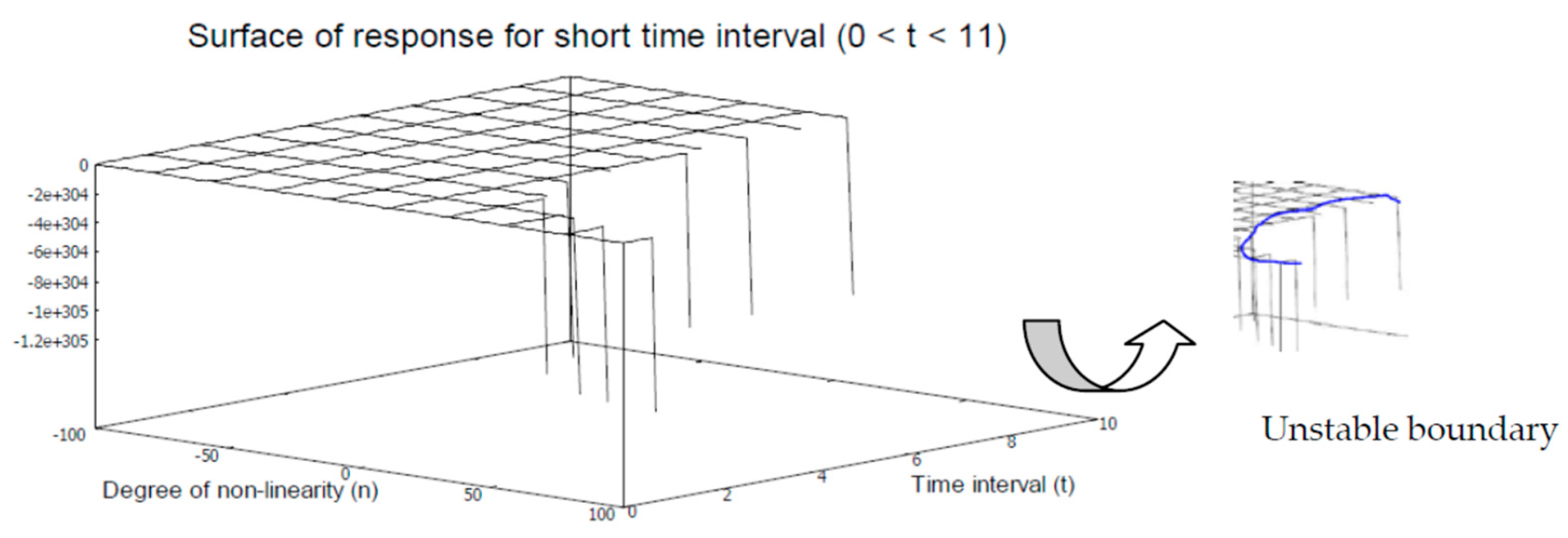
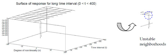
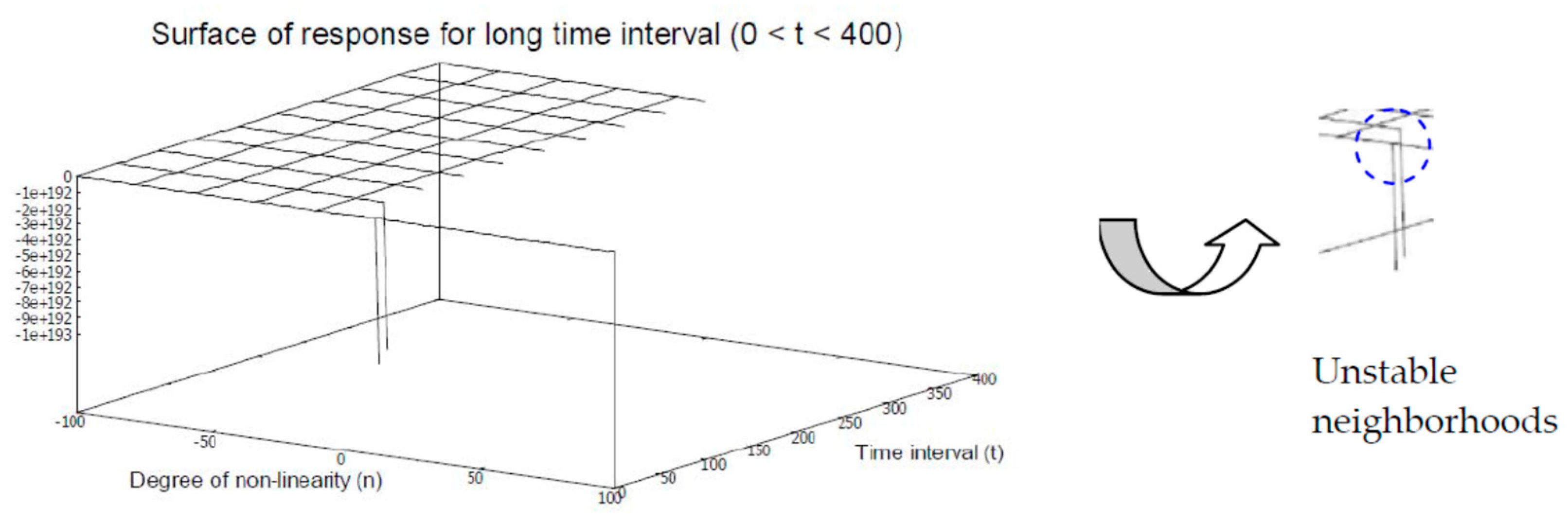
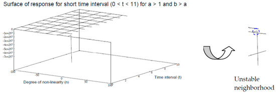
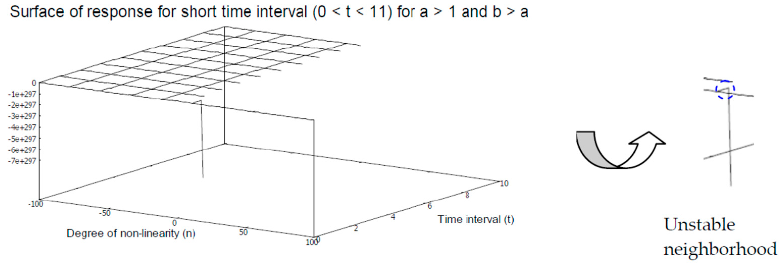
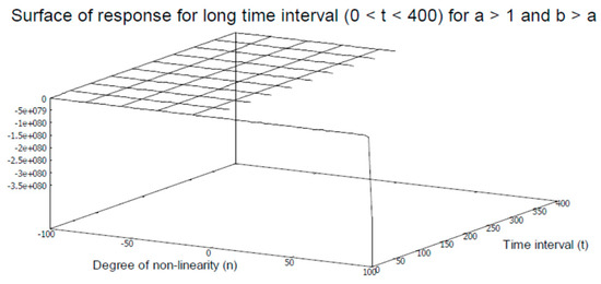
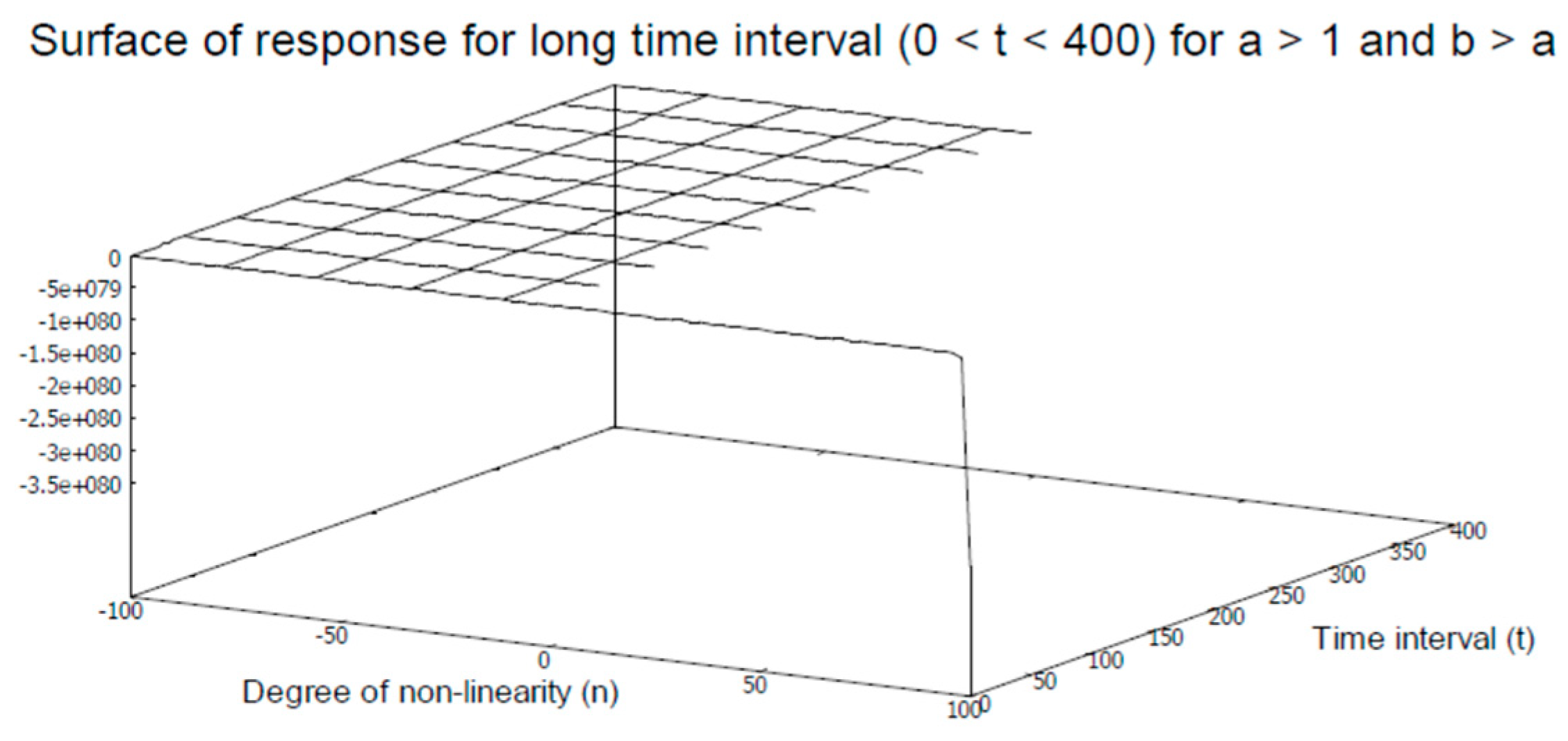
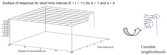
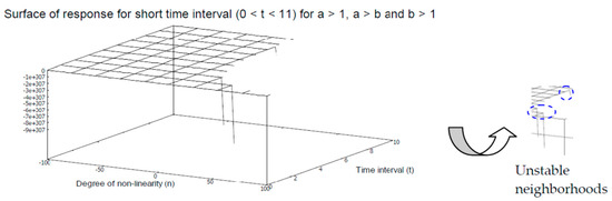
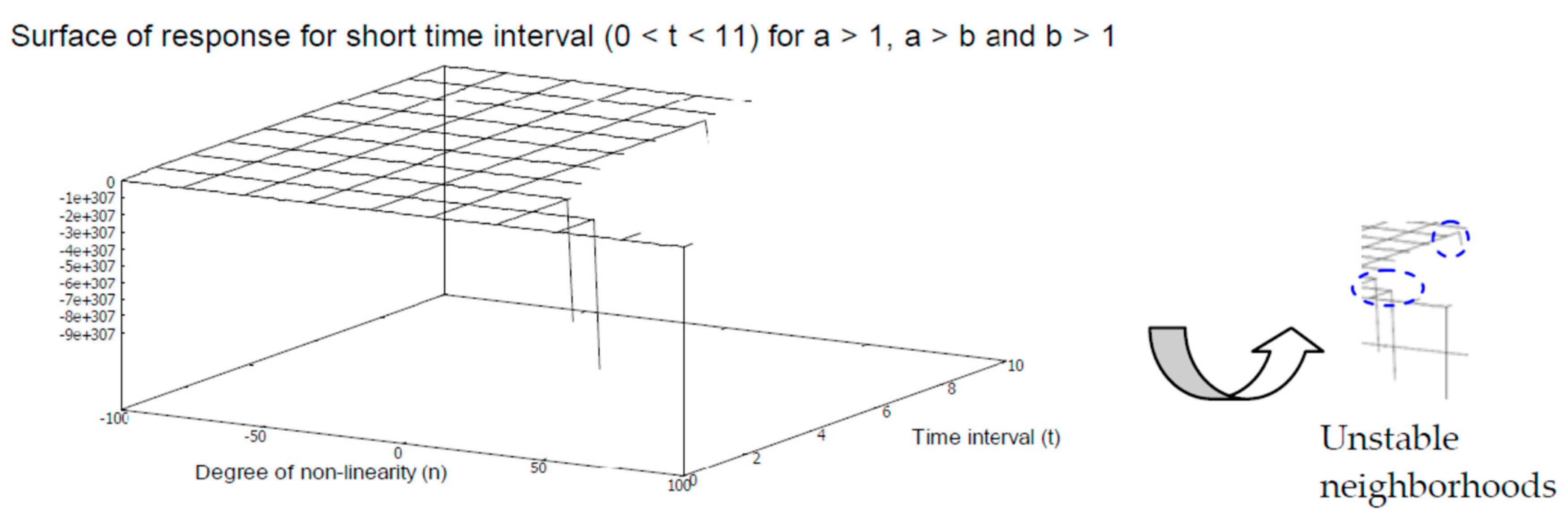
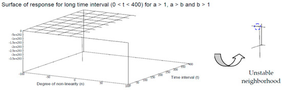
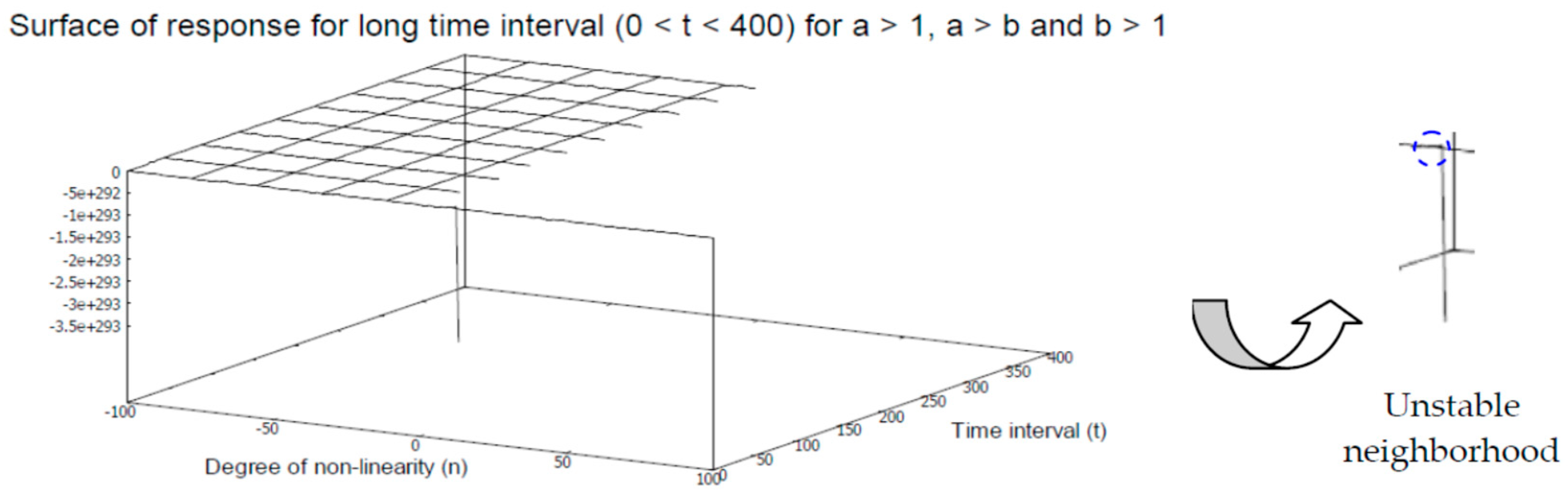
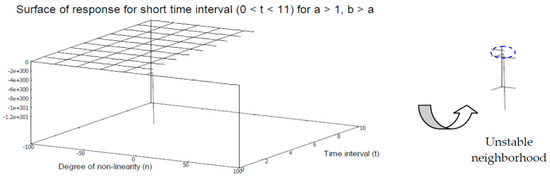
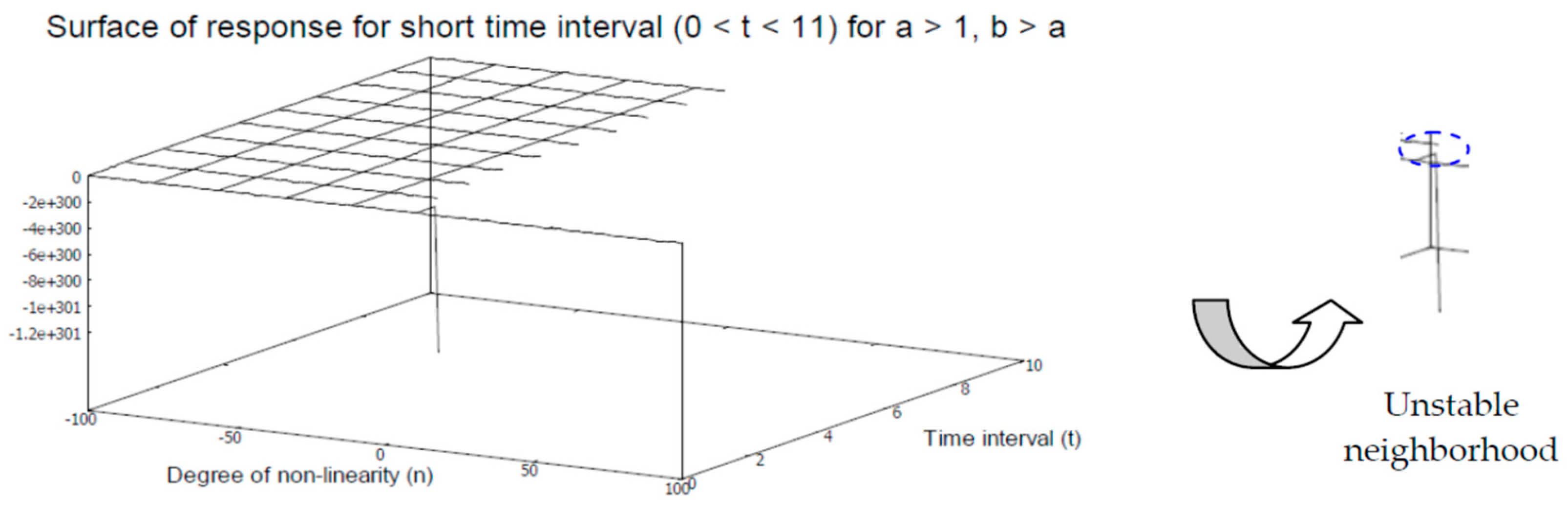
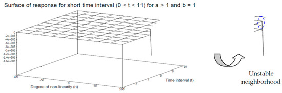
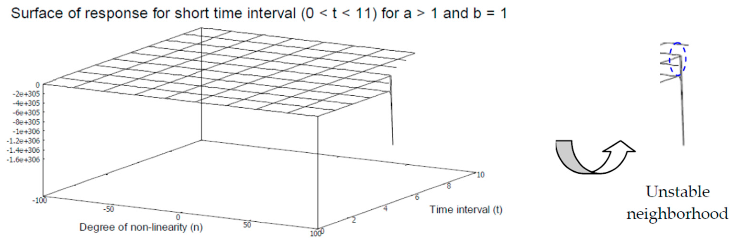
The simulations are performed through numerical computation, where time ($t$) is varied in the two different half-open intervals. In one set of simulations, the time interval is kept very short within the solution space to evaluate the local response profiles. In another set of simulations, the time interval is comparatively larger (the supremum is more than 10 times larger) to evaluate the global response profiles of the ODE under consideration. As a result, if the time, $t$, is fixed in the interval $(0,11)$, then the generated responses are called local responses of the ODE. On the other hand, if time $t$ is varied in the interval $(0,400)$, then the generated responses of the ODE are called global responses. The simulations are performed in three categories based on the values of the constant factor $k\in \{1,h,w\}$, where $h\in R\backslash [0,+\infty )$ and $w\in (1,+\infty )$. The other constants, such as $a,b$, are varied as a relationally ordered pair $(a\Delta b)$ considering various ordering relations, such as $\Delta \in \{\ne ,<,>,=\}$. In all the cases, the degree of non-linearity ($n$) of variable $x$ is varied in the interval $[-100,100]$, covering a wide range in both positive and negative domains. The response profiles of $x(t)$ are presented for various numerical values of the constants and the mutual algebraic relations between them considering the homogeneous form, where the response of ODE at $t=0$ is trivially computable and is not emphasized in the corresponding response profiles. The response profiles are presented as 3D surface maps, where the X-axis represents time, the Y-axis represents the degree of non-linearity, and the variations in the responses of $x(t)$ are given by the Z-axis. The computable regions are presented as surface maps, where the instabilities or singularities in responses are visible at specific neighborhoods within the solution spaces at boundary regions.

3.1. Response Profiles for $k=1$ and $a\ne b$

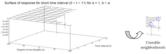
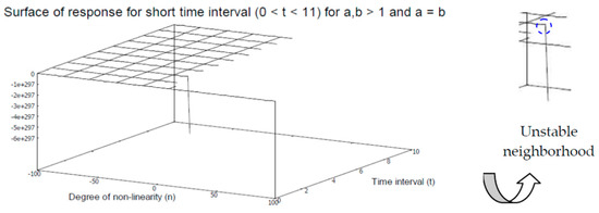
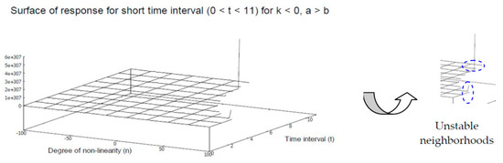
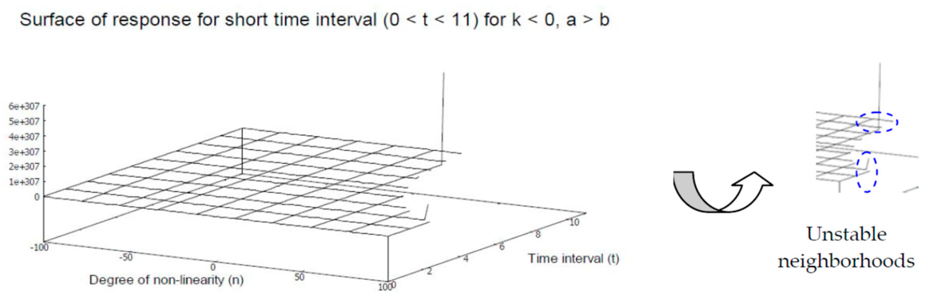
In the first set of simulations, we consider that $k=1$, while the other constant factors are kept finite but unequal within the solution space. The generated 3D response profile is presented in Figure 1 as a surface map for the varying degrees of non-linearity.

Figure 1. Surface map of local response for $k=1, a=1, b=10$.

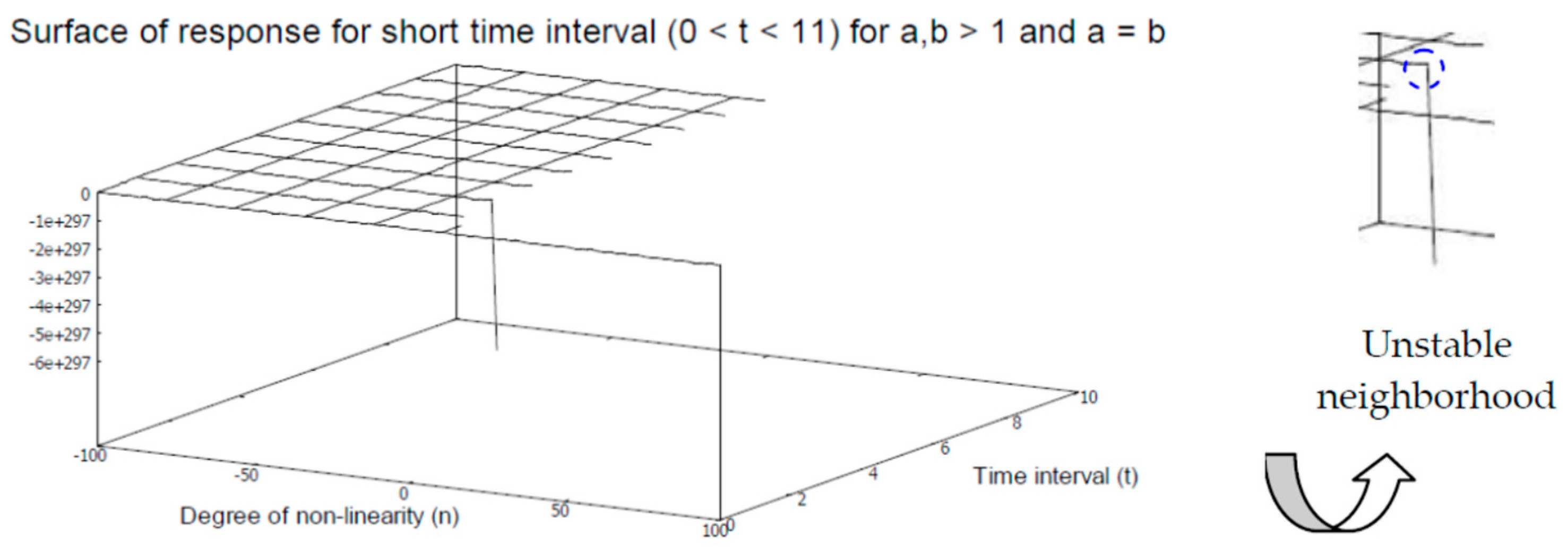
The surface map illustrates that the local response is uniformly flat in the interior of the solution space, thus signifying extreme smoothness for the negative values of non-linearity. However, there are several neighborhoods wherein the local responses attain instabilities in the solution space when the degree of non-linearity is increased more towards the positive domain. The corresponding global response profile is presented in Figure 2.

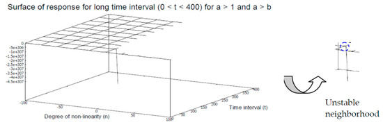
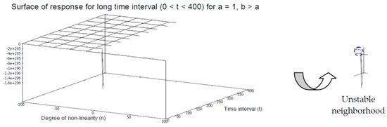
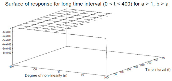
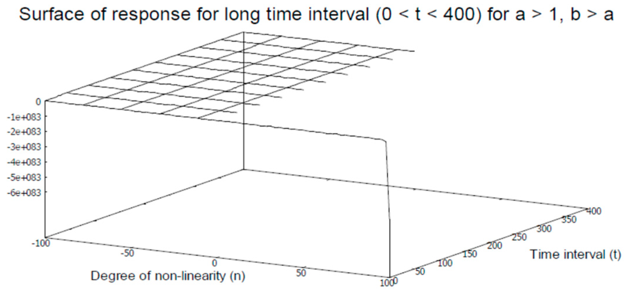
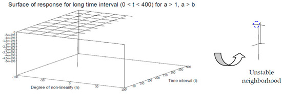
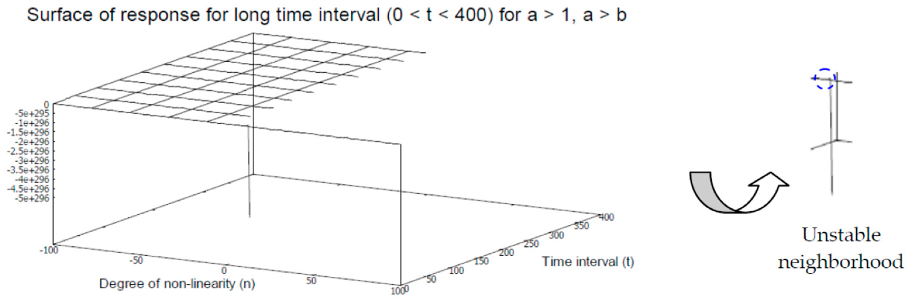
Figure 2. Surface map of global response for $k=1, a=1, b=10$.

It is observable that the global response profile preserves the local response due to the fixed values of the constants and their mutual algebraic relation (an inequality relation in this case). Note that the simulations in these cases consider $a=k$, and the algebraic ordering is $b>a$. If we relax the restriction on one of the constants such that $a>1$ while enhancing the values of another constant 10 times compared to the earlier case, then the generated local response profile retains smoothness, as presented in Figure 3. Interestingly, in this case, the local response profile is comparable to the global response with constrained values of the constants, as given in Figure 2.

Figure 3. Surface map of local response for $k=1, a=7, b=100$.

The surface map of the global response profile with $a>1$ and $b>a$ is illustrated in Figure 4. The global response profile retains local smoothness, and the boundary of the solution space is sharp near the origin, which contrasts with the earlier 3D surface maps.

Figure 4. Surface map of global response for $k=1, a=7, b=100$.

Interestingly, if we reverse the combinatorial selection of the constants such that $k=1, a=10, b=1$, then the 3D surface map of local response profile is extended into the positive domain of non-linearity, as presented in Figure 5. Note that in this case, the smoothness is preserved for an extended interval within the solution space and the neighborhood of instability is confined within a narrow zone at a comparatively higher time interval.

Figure 5. Surface map of local response for $k=1, a=10, b=1$.

The corresponding global response profile is illustrated as the surface map given in Figure 6. The pronounced effect of non-linearity is observable in the global response profile as compared to the local response profile, wherein the values of the constants remain unaltered. The location of the neighborhood of instability is also shifted closer to the origin, where the boundary of the solution space is sharp.

Figure 6. Surface map of global response for $k=1, a=10, b=1$.

However, the local response profile of the ODE is moderately altered if we increase one of the constants as $b>1$ while keeping $k=1$. The corresponding 3D surface map is shown in Figure 7. It is relatively clear to see that smoothness is retained mostly in the negative index of non-linearity and that there are instabilities at the boundary region for the increased degree of non-linearity in the positive domain.

Figure 7. Surface map of local response for $k=1, a=100, b=7$.

On the contrary, the global response profile exhibits a retraction mode if we increase the time interval while keeping all other parameters unaltered. This observation is depicted in Figure 8. The neighborhood of instability is present in the surface map very close to origin.

Figure 8. Surface map of global response for $k=1, a=100, b=7$.

The comparisons of the surface maps illustrate that the response profiles of the ODE in Figure 3, Figure 6, and Figure 8 are nearly comparable. This indicates that the effects of the combinatorial choices of the constants $a,b$ determine the dynamics of the local and global responses for the fixed value of $k=1$ (i.e., in the positive domain closer to the origin).

3.2. Response Profiles for $k>1$ and $a\ne b$

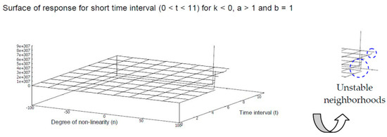
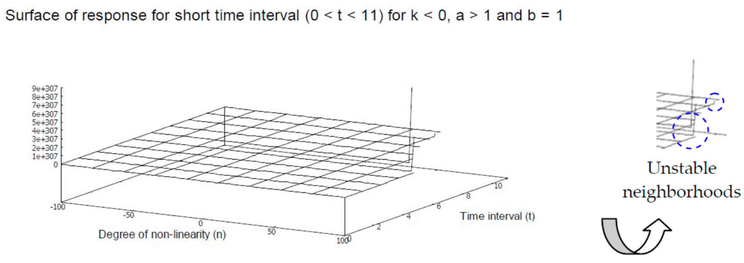
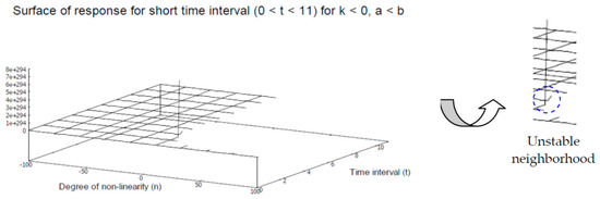
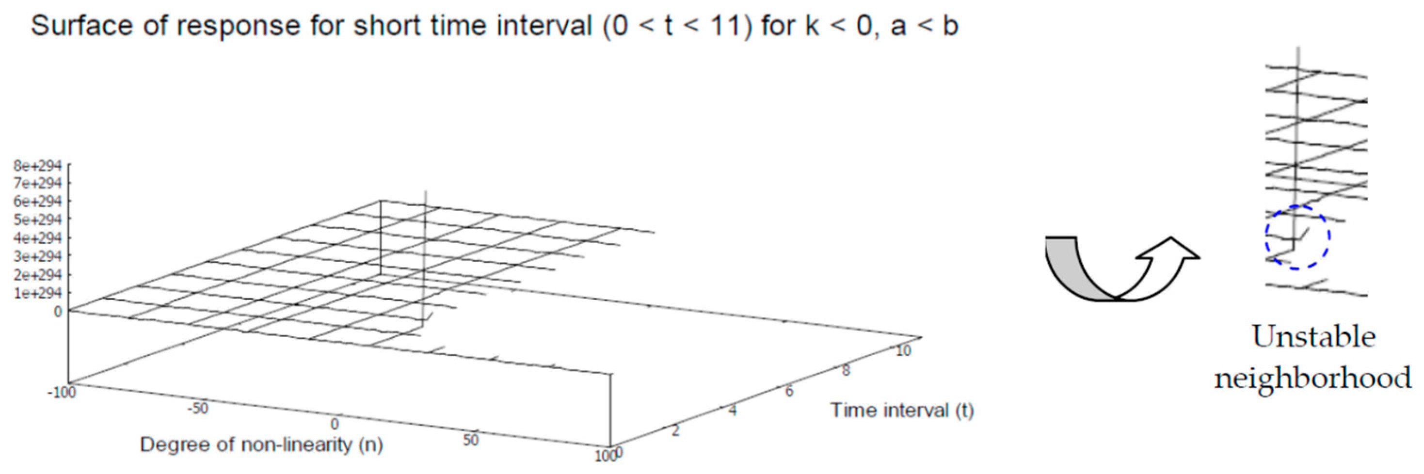
The simulation results presented in this section illustrate the effects of increasing the value of $k$ in the positive domain away from origin. The 3D surface map of the local response profile for $k=40, a=1, b=10$ is given in Figure 9. The comparisons of the response profiles given in Figure 1 and Figure 9 show that the increasing value of $k$ reduces the neighborhoods of instabilities within the solution space.

Figure 9. Surface map of local response for $k=40, a=1, b=10$.

Interestingly, the comparisons of the global response profiles given in Figure 2 and Figure 10 show that the surface maps are nearly similar in both cases. This indicates that at longer time intervals, the effect of the moderately increased value of $k$ is negligible.

Figure 10. Surface map of global response for $k=40, a=1, b=10$.

Likewise, if the values of constants $a,b$ are increased while maintaining the algebraic ordering relation $b>a$, then the surface map of the local response profile, represented in Figure 11, remains nearly identical to that of Figure 10. This indicates that the values of the respective constants do not heavily influence the response when the corresponding algebraic ordering relation is maintained.

Figure 11. Surface map of local response for $k=40, a=7, b=100$.

The global response profile of the ODE under consideration is largely similar to those of Figure 10 and Figure 11, except for the elimination of instabilities at the boundary regions, as shown in Figure 12.

Figure 12. Surface map of global response for $k=40, a=7, b=100$.

The similarity between Figure 4 and Figure 12 suggests that the global response of the ODE is stable under the corresponding choices of the constants $a,b$ and the algebraic ordering $b>a$ and that it is not sensitive to the values of $k$.

The noticeable shift in the local response profile of the ODE is observable if the algebraic ordering relation between constants is changed to $a>b$. The corresponding 3D surface map of the response profile is shown in Figure 13. Note that the response surface largely covers both positive and negative domains of varying degrees of non-linearity (i.e., an expansion of a uniformly stable solution space emerges). The neighborhood of instability is locally restricted at the sharp boundary region.

Figure 13. Surface map of local response for $k=40, a=10, b=1$.

The global response profile of the ODE with an algebraic ordering of constants of $a>b$ and a value of $k=40$ is given in Figure 14. Interestingly, it is nearly identical to the responses shown in Figure 3, Figure 6, Figure 8, and Figure 11. This observation illustrates that both the local and global dynamics of the ODE under consideration are highly stable irrespective of the combinatorial effects exerted by the set of constants $\{a,b,k\}$.

Figure 14. Surface map of global response for $k=40, a=100, b=7$.

3.3. Response Profiles for $k>1$ and $a=b$

The results of the numerical simulation presented in this section compute the global and local response profiles of the ODE under periodic DD forcing, while the parameters are set as $a,b,k\in (1,+\infty )$ and the algebraic restriction is enforced as $a=b$. The corresponding local response profile is presented in Figure 15.

Figure 15. Surface map of local response for $k=40, a=b=100$.

The surface map of the local response of the ODE appears to be fairly smooth and uniform with a varying degree of non-linearity. However, the neighborhood of instability is observable within the solution space. Interestingly, if we compute the global response of the ODE in a relatively longer time interval, then the uniformity and smoothness of the surfaces are retained within the sharp boundary, as presented in Figure 16.

Figure 16. Surface map of global response for $k=40, a=b=100$.

Notably, the response surfaces are not computable when covering the entire region of the varying degree of non-linearity. In other words, the global and local response profiles appear to be incompletely identical across the large solution space under the parameters applied in this case.

However, if we reverse the sign of $k$ into the negative domain, then the influence of the degree of varying non-linearity is reduced and the response surfaces are extended, as presented in the following section.

3.4. Local Response Profiles for $k<0$

In this section, we present the local response profiles of the ODE, while reversing the sign of $k$ into the negative domain away from the origin and fixing the constant $b=1$. However, the other constant is changed to $a\in (1,+\infty )$. The corresponding local response profile is presented in Figure 17, where $a=10$. It is easily observable that the uniform solution space free of instability is expanded. The oriented instabilities appear in multiple local neighborhoods at sharp boundary regions.

Figure 17. Surface map of local response for $k=-40, a=10$.

Next, we increase the value of constant $b$ such that $b=30$ (i.e., three times greater than the earlier value of constant $a$), and we reduce the value of constant $a$ such that an algebraic relation wherein $a<b$ is enforced. As a result, the effect of the varying degree of non-linearity is observable in the local response profile, as presented in Figure 18. Note that the space of uniformity and smoothness of the surface has contracted. This indicates that the choices of the values of the constants and the algebraic ordering have effects on the local response of the ODE under periodic DD forcing.

Figure 18. Surface map of local response for $k=-40, a=4, b=30$.

Finally, we reverse the algebraic ordering relation of constants $\{a,b\}$ again and we keep the value of constant $k$ unaltered in the negative domain. The corresponding local response profile is presented in Figure 19.

Figure 19. Surface map of local response for $k=-40, a=10, b=2$.

Observe that the space with a stable response is expanded, covering widely varying degrees of non-linearity unlike the earlier case. However, the neighborhoods of instabilities at the boundary within the solution space are observable in the response profile.

3.5. Evaluations of Variations of Sum of Series

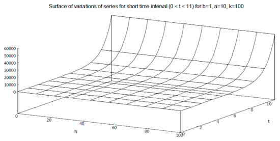
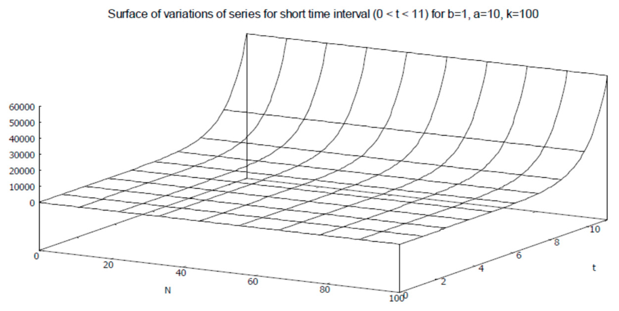
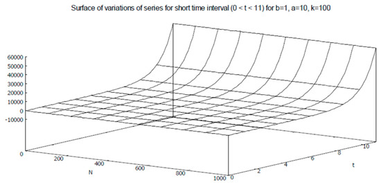
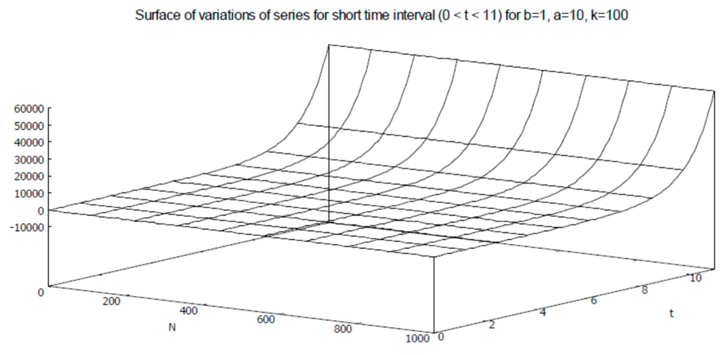
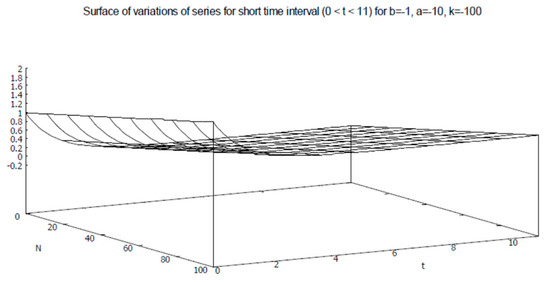
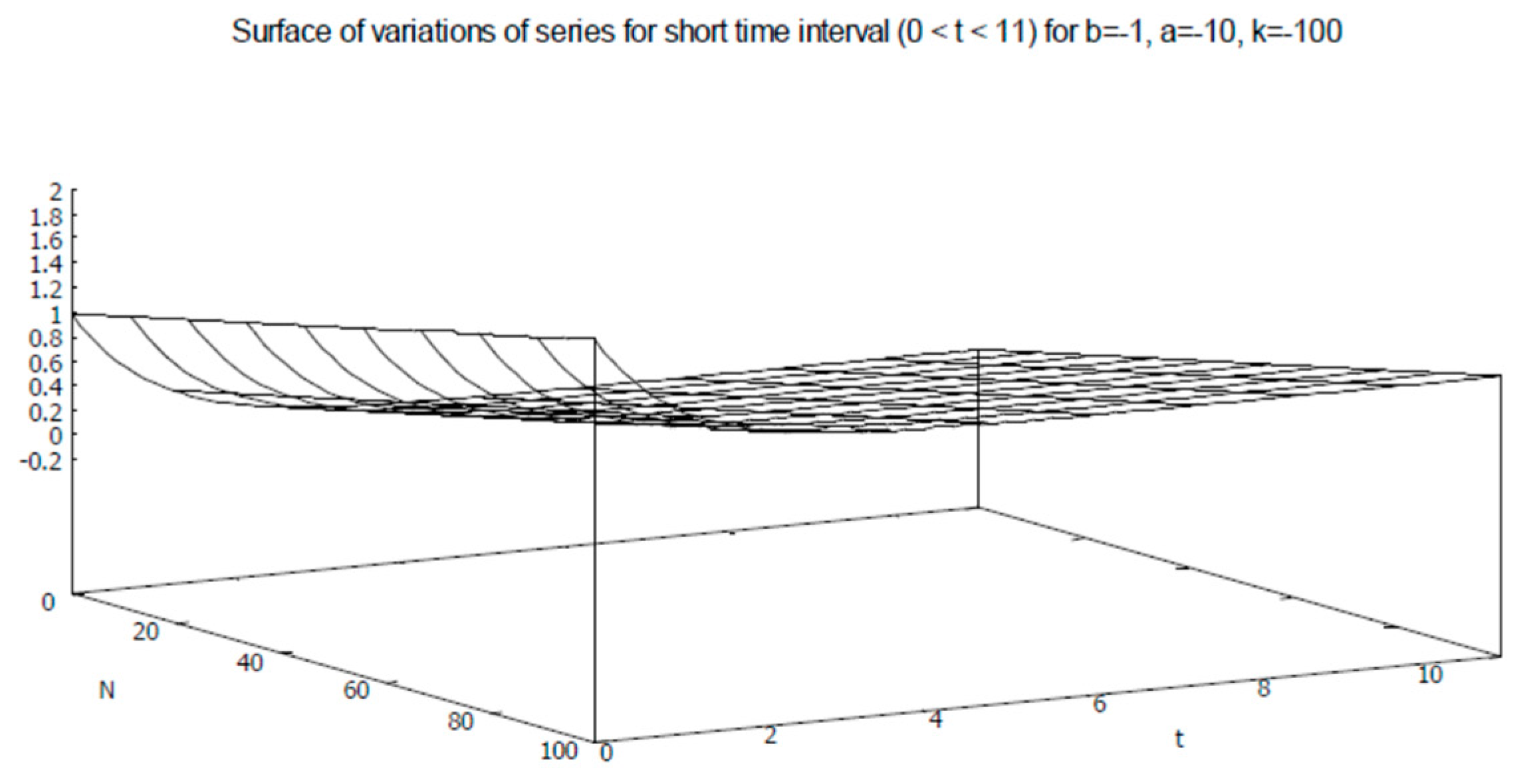
In this section, we present the variations of the sum of series ${\displaystyle {\sum }_t(1+{\epsilon }_t)}$ as given in Equation (9) with respect to the variations of $t,N$ and the degree of non-linearity ($n$). The variations of the sum of series are presented on the Z-axis. First, we show that the sum of series is bounded for the second degree of non-linearity, the short range of series $N=[0,100]$, and the positive values of the elements of the set $\{a=10, b=1, k=100\}$. The resulting response profile is given in Figure 20.

Figure 20. Surface map of local variations of ${\displaystyle {\sum }_t(1+{\epsilon }_t)}$ (on Z-axis) for $n=2$.

Next, we increase the range of series to a relatively large value such that $N=[0,1000]$ while keeping the other parameters unchanged. The resulting response profile is presented in Figure 21. It is interesting to note that the enhancement of the range of series does not have any large influence on the response profile.

Figure 21. Surface map of local variations of ${\displaystyle {\sum }_t(1+{\epsilon }_t)}$ (on Z-axis) for $N=[0,1000]$.

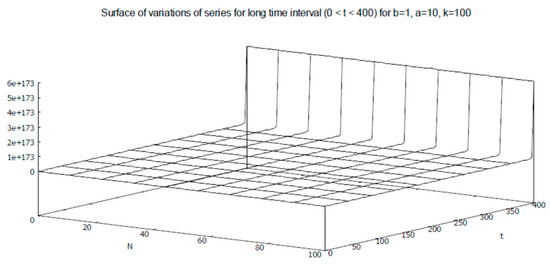
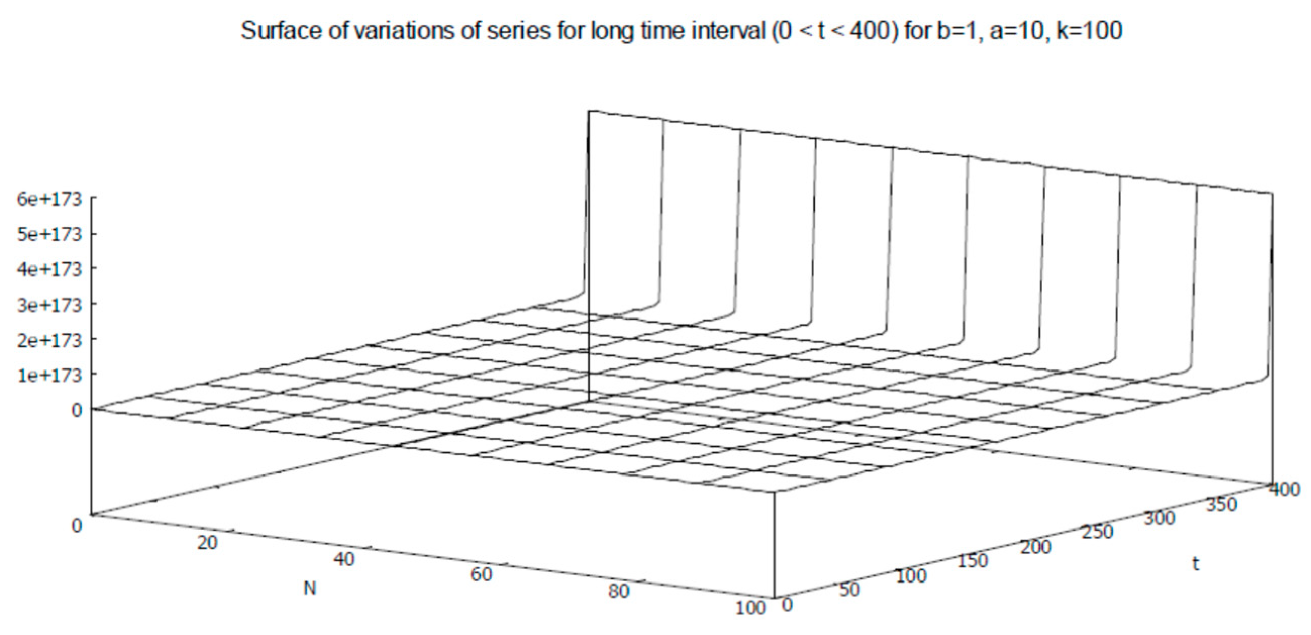
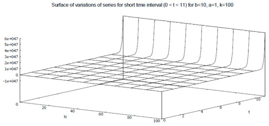
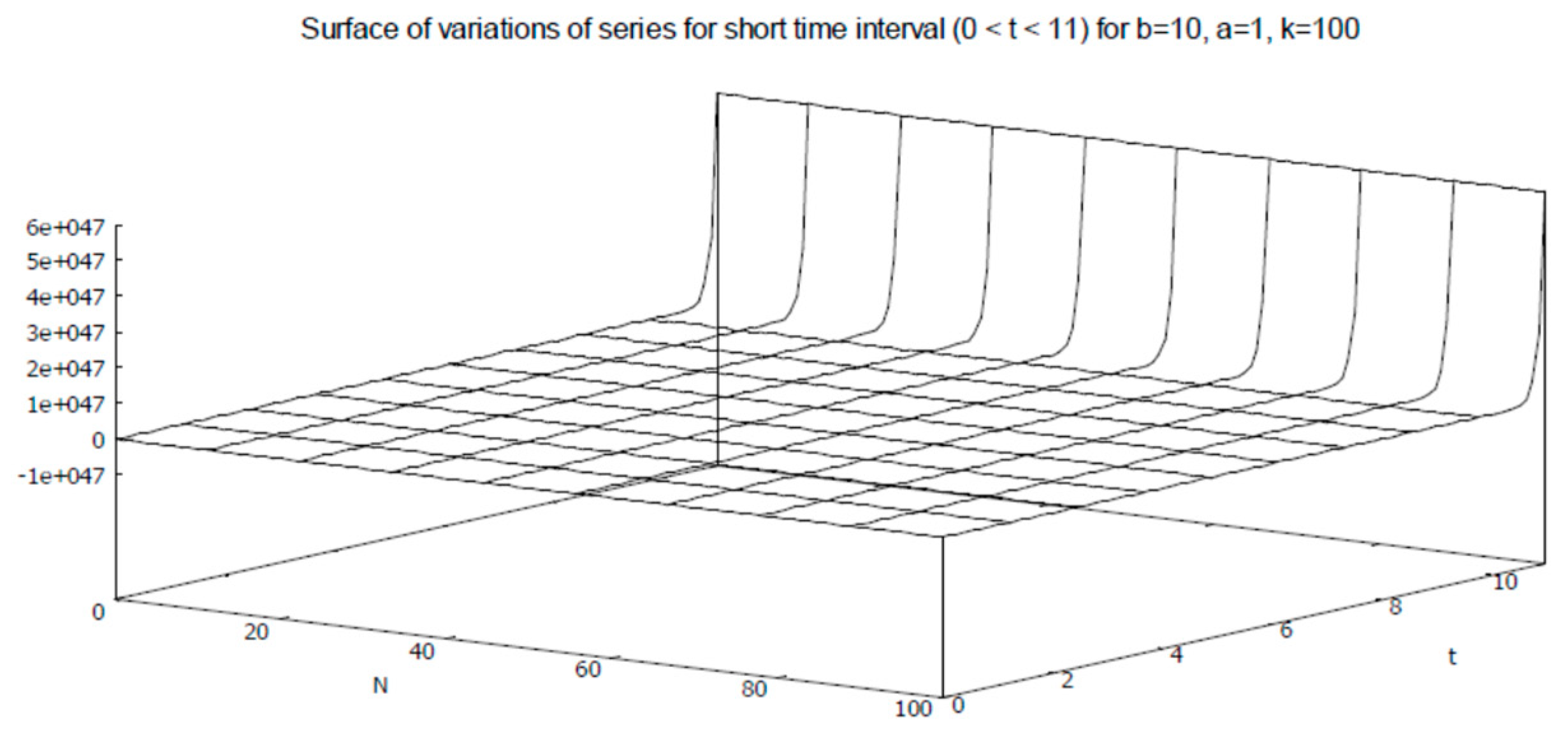
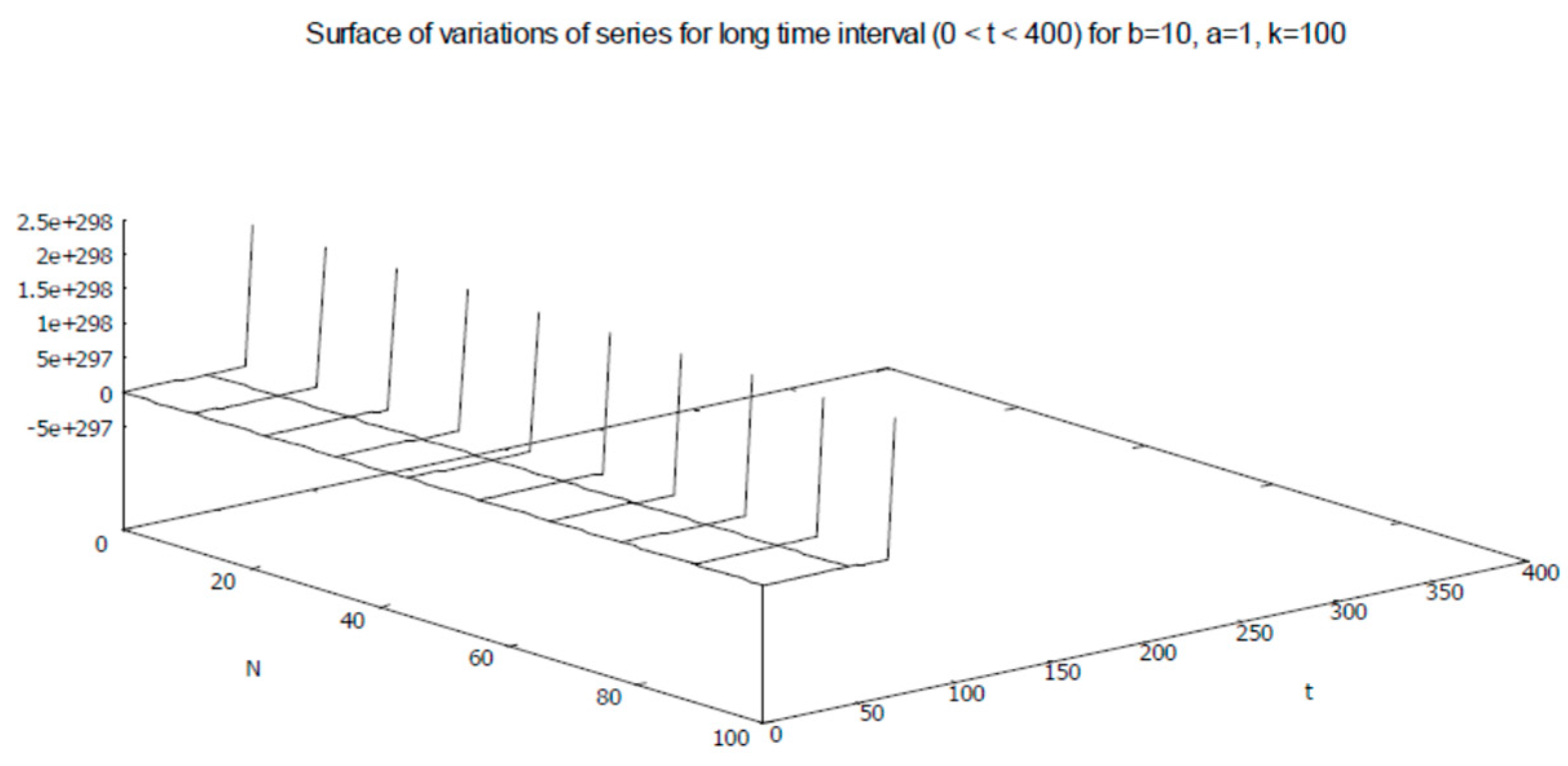
In the next experiment, we reduced the range of the series and computed the global response profile, and the results are given in Figure 22. The rapid increase in the values of the sum of the series is observable at the sharp boundary.

Figure 22. Surface map of global variations of ${\displaystyle {\sum }_t(1+{\epsilon }_t)}$ for $N=[0,100]$, $n=2$.

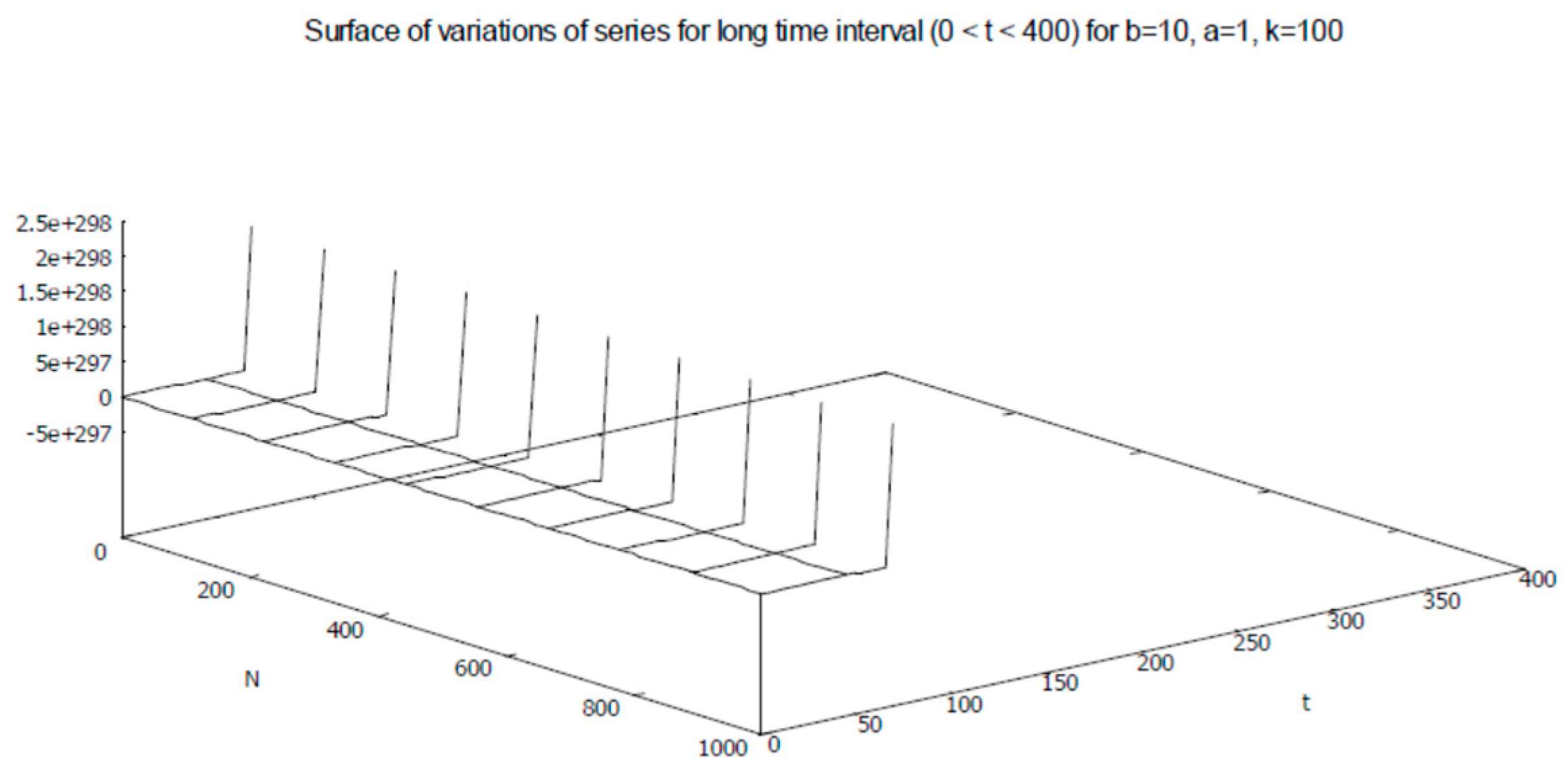
A similar effect is sustained in the global response profile if we enhance the range of the series by ten-fold, as presented in Figure 23.

Figure 23. Surface map of global variations of ${\displaystyle {\sum }_t(1+{\epsilon }_t)}$ for $N=[0,1000]$, $n=2$.

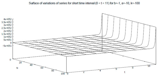
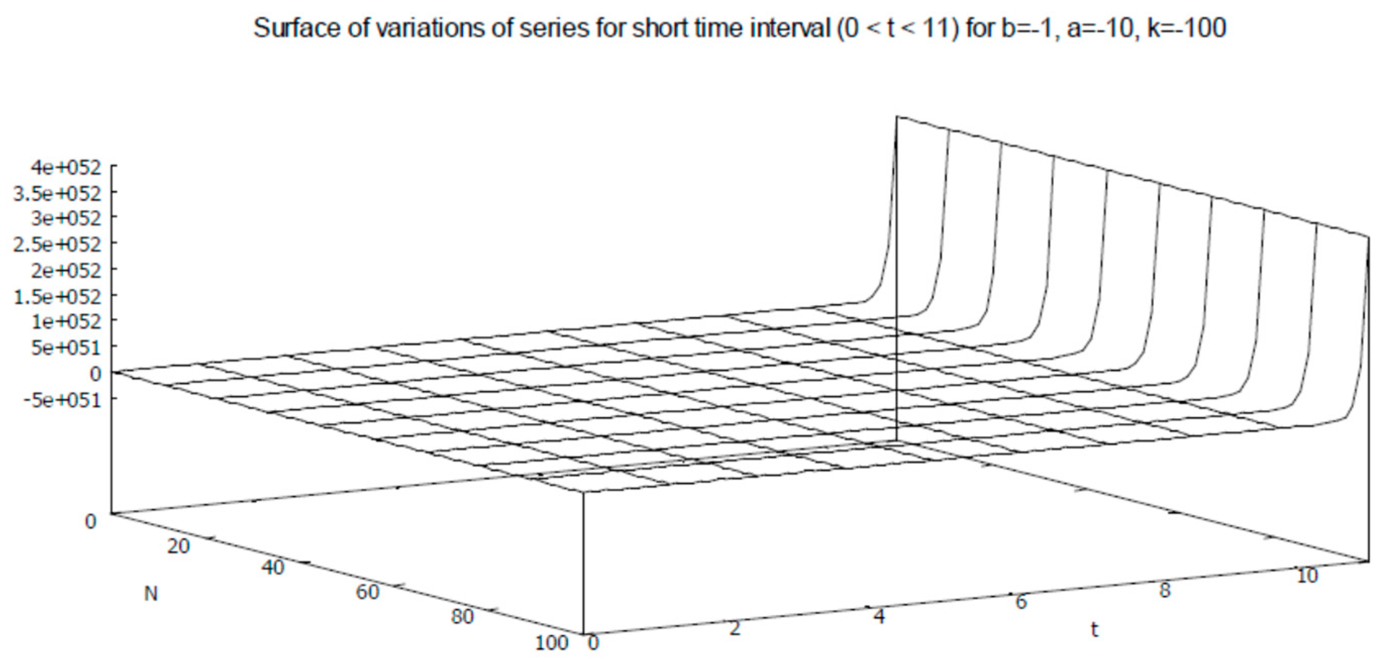
However, the increase in the values of the sum of the series becomes relatively gradual if we rearrange the combinatorial values of constants such that $\{a=1, b=10, k=100\}$. The resulting response profile is given in Figure 24.

Figure 24. Surface map of local variations of ${\displaystyle {\sum }_t(1+{\epsilon }_t)}$ for $N=[0,100]$ and $n=2$.

An observable shift in the variations in the sum of the series appears if the global response profile is computed for a relatively short range of the series, i.e., $N=[0,100]$. The resulting response profile is presented in Figure 25.

Figure 25. Surface map of global variations of ${\displaystyle {\sum }_t(1+{\epsilon }_t)}$ for $N=[0,100]$ and $n=2$.

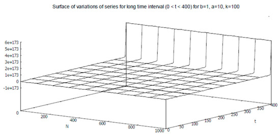
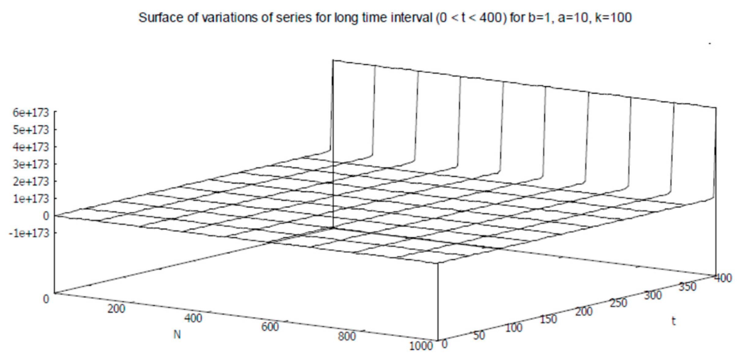
Interestingly, the aforesaid shift in the response is retained, as presented in Figure 26., even if we increase the range of the series to ten times that of the earlier experiment. Note that the degree of non-linearity remains unchanged.

Figure 26. Surface map of global variations of ${\displaystyle {\sum }_t(1+{\epsilon }_t)}$ for $N=[0,1000]$ and $n=2$.

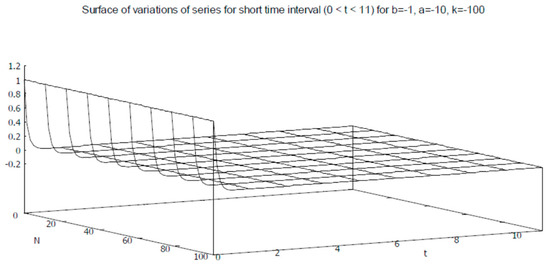
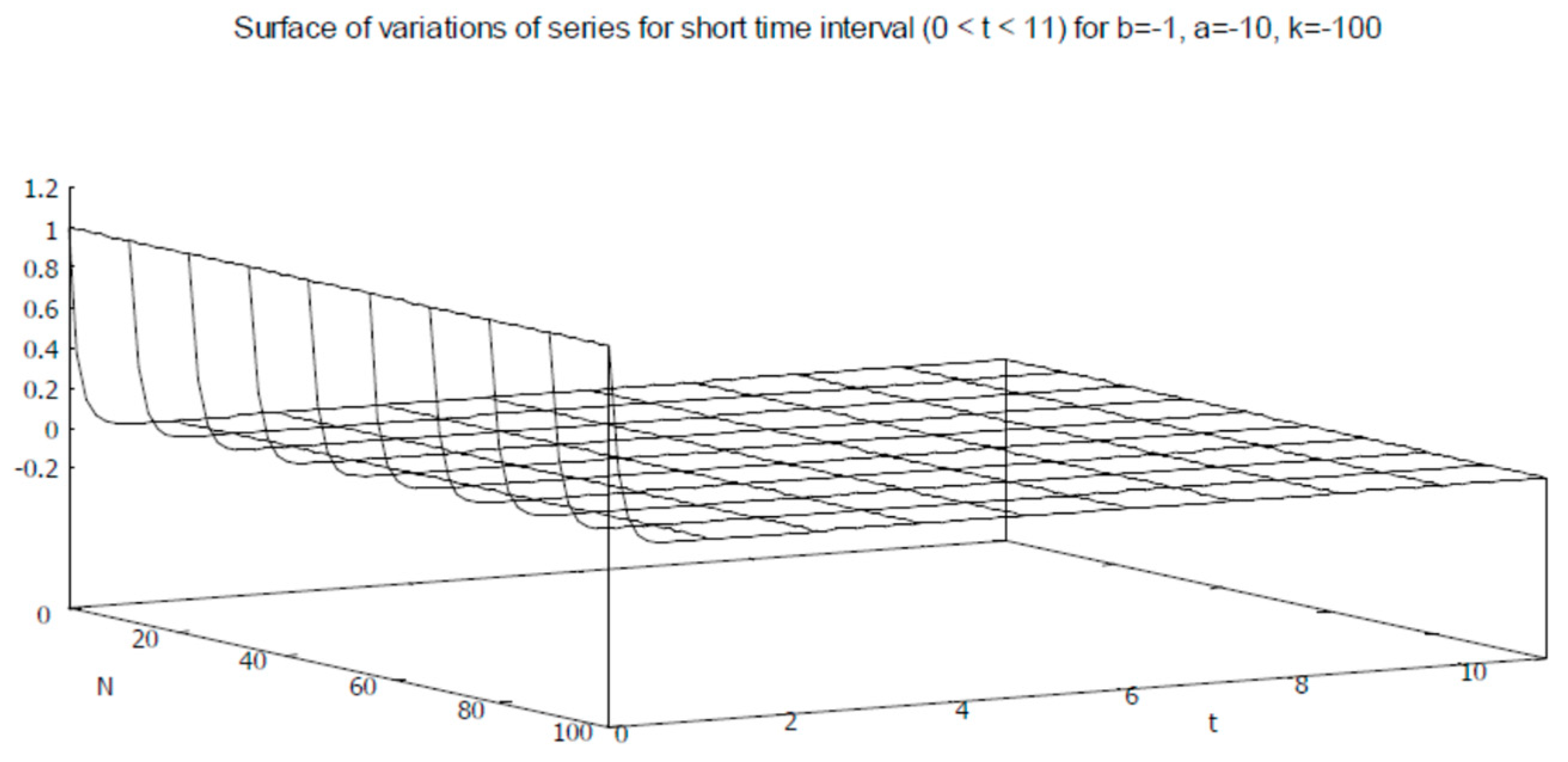
In the next experiment, we make combinatorial changes to the set of constants such that $\{a=-10,b=-1,k=-100\}$. This reverses the domain of the set of constants from positive to negative. The resulting response profile is presented in Figure 27. Interestingly, the influence of the domain of the set of constants is visible in the response profile, where the sum of series shows a gradual decline to a stable surface.

Figure 27. Surface map of local variations of ${\displaystyle {\sum }_t(1+{\epsilon }_t)}$ (on Z-axis) for $N=[0,100]$, $n=2$.

The slope of the reduction in the values of the sum of series becomes steeper than that of the previous response if we increase the degree of non-linearity five times in the positive domain. The resulting response profile is shown in Figure 28.

Figure 28. Surface map of local variations of ${\displaystyle {\sum }_t(1+{\epsilon }_t)}$ for $N=[0,100]$ and $n=10$.

The effect of the degree of non-linearity on the series is observable (Figure 29) when we change the degree of non-linearity from the positive domain to the negative domain.

Figure 29. Surface map of local variations of ${\displaystyle {\sum }_t(1+{\epsilon }_t)}$ for $N=[0,100]$ and $n=-10$.

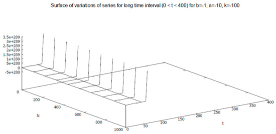
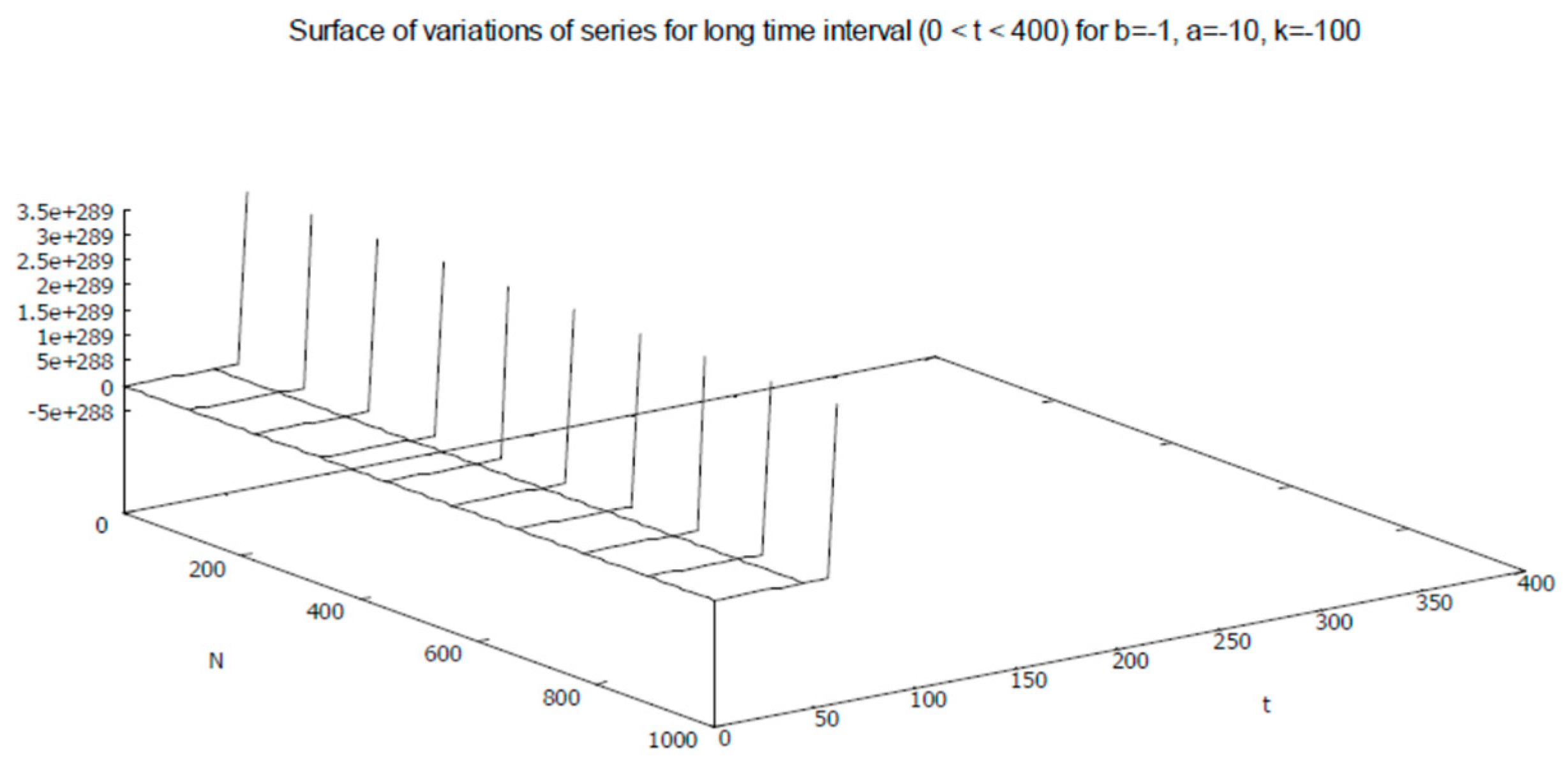
On the other hand, the response profile of the sum of series shows sensitivity with respect to the range of the series. This effect is visible in Figure 30.

Figure 30. Surface map of global variations of ${\displaystyle {\sum }_t(1+{\epsilon }_t)}$ for $N=[0,1000]$ and $n=-10$.

Evidently, the overall effects of the domain of non-linearity and the domains of the constants on the variations of the sum of series are significantly different. However, in all cases, the variations are finite. Moreover, the mutual variations of the domain of non-linearity and the range of the series have greater effects on the response profiles.

4. Applicational Prospects

In this section, the applicational prospects of the differential equations with discontinuous forcing are presented, and the distinguishing properties of the proposed approach are outlined comprehensively. In general, the ODEs involving sporadic disturbances have applications in fluid-flow modeling, wherein the uncertainties are considered to be the governing factors of the respective dynamics [13]. ODEs and PDEs (Partial Differential Equations) with Dirac delta forcing have a wide array of applications in physical sciences and engineering [14]. For example, the one-dimensional and two-dimensional differential equations equipped with Dirac-type discrete forcing are given as $-u_{xx}=\delta (x-a), a\in R$ and $-{\nabla }^2{u}_{xy}=\delta (x,y)$, respectively, with applications in geology and hydrology [14,15]. On the other hand, the non-homogeneous ODE in the form given in Equation (1) has potential applications in the jitter modeling of networked systems [16,17,18]. Specifically, in computer network modeling involving sporadic jitters, the constant factor is considered to be positive (i.e., $k>0$). The main focus of the analysis of such differential equations with discontinuous forcing is to ascertain the convergence in the solution spaces and the rapidity of such convergence [19]. In general, the ODEs of perturbed systems consider uniform convergence of solutions within $[a,b]$, where the solution intervals are finite in the set of reals $R$. Let us consider that the forcing factor $f(.)$ is restricted to relative smoothness (i.e., the forcing $f\in C^3([a,b]$) for a singularly perturbed system [19]. This indicates that the governing equations of such systems do not consider discontinuities in the forcing factors. As a distinction, the analyses presented in this paper consider periodic discontinuities in the forcing function $f(.)$. Furthermore, the positions of the roots of characteristic equations do not play any significant role with respect to maintaining generality, as proposed in this paper. The modeling of systems with input disturbances considers cascaded PDE-ODE formulation given by $DX=AX(t)+Bu(0,t)$ with the condition $u_x(1,t)=U(t)+\omega (t)$, where $U(t)$ is the control input, $\omega (t)$ is the disturbance within input, $A$ is an $n\times n$ constant matrix, and $B$ is an $n\times 1$ constant matrix [20]. It is important to note that the elements of constant matrices $A,B$ are real numbers such that the ordered pair $(A,B)$ is stabilizable. The formulation depends on the precondition that $\omega (t)$ can be resolved as $\omega (t)={\displaystyle \sum _i{f}_i(t)}$, where every $f_i(t)$ is periodic and $i\in [1,m], m<+\infty$. Furthermore, it is required that $|f_i(t)|<+\infty$ in the system under consideration. The distinctive property of the algebraic analyses proposed in this paper is that the forcing factor is periodic as well as discontinuous and does not specially distinguish any control input $U(t)$ separately. Moreover, the resolution of periodic forcing does not require the convergent finite sum of other periodic functions within a finite interval (i.e., we are not decomposing Dirac forcing into external function forms). In other words, our proposed algebraic analyses consider a generalized analytical formulation. Note that numerical solution approaches are frequently employed rather than complete analytical methods in order to avoid complexities. It has been observed that numerical solution approaches are prone to the effects of varying dimensionalities [14,19]. In such cases, the convergence analyses deal with the limiting value property ${\delta }_{\epsilon }\to \delta ,\epsilon >0$ through the regularization of the discrete delta function ${\delta }_{\epsilon }$ towards the Dirac delta forcing. However, the algebraic and numerical analyses presented in this paper are in a general form that does not require any specific regularization.

5. Conclusions

Second-order, non-homogeneous ODEs with both discontinuous and periodic forcing have numerous applications in engineering sciences as well as computational sciences. Second-order ODEs equipped with Dirac delta forcing comprise a variety of this class of equations. Analyses of such equations are difficult in multi-dimensional cases and the complexities are increased if the number of variables with discontinuities is increased. In order to analyze such equations, Lipschitz regularizations and Lebesgue measurability conditions are often employed. The generalized analytical approach presented in this paper was conducted with two directions: conducting algebraic analyses of convergence in lower-dimensional cases in simple forms under Dirac delta forcing and determining the corresponding numerical simulations of the behaviors of the solution spaces. The algebraic analyses proposed in this paper do not assume any specific preconditions or pre-regularizations. It has been shown that locally finite and smooth responses are admissible within exponential solution spaces and that discontinuous forcing can be resolved. Numerical simulations exhibit a set of consistent local uniformities in solution spaces. However, the global response profiles show occasional appearances of oriented discontinuities at specific local neighborhoods in the solution spaces with sharp boundaries. The expansion–contraction of smooth and uniformly stable response profiles is observable depending on the chosen sets of parameters and time intervals influencing the governing equation. The analyses proposed in this paper consider the sequential convergence property within the solution spaces, without requiring any relative smoothness of the forcing function.

References

- Precup, R.; Rodríguez-López, J. Positive solutions for ϕ-Laplace equations with discontinuous state-dependent forcing terms. Nonlinear Anal. Model. Control 2019, 24, 447–461. [Google Scholar] [CrossRef] [Scilit]
- Brauer, F. Nonlinear Differential Equations with Forcing Terms. Proc. Am. Math. Soc. 1964, 15, 758–765. [Google Scholar] [CrossRef]
- Walsh, J.; Widiasih, E. A discontinuous ODE model of the glacial cycles with diffusive heat transport. Mathematics 2020, 8, 316. [Google Scholar] [CrossRef] [Scilit]
- Filippov, A.F. Differential Equations with Discontinuous Righthand Sides; Kluwer Academic Publishers: Dordrecht, The Netherlands, 1988. [Google Scholar]
- Hajek, O. Discontinuous differential equations. J. Diff. Eqn. 1979, 32, 149–170. [Google Scholar] [CrossRef] [Scilit]
- Eich-Soellner, E.; Führer, C. Integration of ODEs with Discontinuities. In Numerical Methods in Multibody Dynamics; Chapter 6; Springer Fachmedien Wiesbaden: Wiesbaden, Germany, 1998. [Google Scholar]
- Gear, C.W.; Osterby, O. Solving Ordinary Differential Equations with Discontinuities. ACM Trans. Math. Softw. 1984, 10, 23–44. [Google Scholar] [CrossRef] [Scilit]
- Lu, C.; Browning, G. Discontinuous forcing generating rough initial conditions in 4DVAR data assimilation. J. Atmos. Sci. 2000, 57, 1646–1656. [Google Scholar] [CrossRef] [Scilit]
- Moreau, J.J.; Panagiotopoulos, P.D.; Strang, G. (Eds.) Topics in Nonsmooth Mechanics; Birkhäuser Verlag: Basel, Switzerland, 1988. [Google Scholar]
- Brogliato, B. Nonsmooth Impact Mechanics. In Models, Dynamics and Control; Springer: London, UK, 1996. [Google Scholar]
- Akhmet, M. Principles of Discontinuous Dynamical Systems; Springer: New York, NY, USA, 2010. [Google Scholar]
- Nedeljkov, M.; Oberguggenberger, M. Ordinary differential equations with delta function terms. Publ. de L’institut Mathématique 2012, 91, 125–135. [Google Scholar] [CrossRef] [Scilit]
- Kumar, V.; Singh, S.K.; Kumar, V.; Jamshed, W.; Nisar, K.S. Thermal and thermo-hydraulic behaviour of alumina-graphene hybrid nanofluid in minichannel heat-sink: An experimental study. Int. J. Energy Res. 2021, 45, 20700–20714. [Google Scholar] [CrossRef] [Scilit]
- Cola, V.S.D.; Cuomo, S.; Severino, G. Remarks on the approximation of Dirac delta functions. Results Appl. Math. 2021, 12, 100200. [Google Scholar] [CrossRef] [Scilit]
- Indelman, P. Steady-state source flow in heterogeneous porous media. Trans. Porous Media 2001, 45, 105–127. [Google Scholar] [CrossRef] [Scilit]
- Cveticanin, L. Strongly Nonlinear Oscillators, 233 Undergraduate Lecture Notes in Physics/L. Cveticanin; Springer International Publishing: Cham, Switzerland, 2016. [Google Scholar]
- Taqqu, M.; Willinger, W.; Sherman, R. Proof of a fundamental result in self–similar traffic modelling. Comput. Commun. Rev. 1997, 27, 5–23. [Google Scholar] [CrossRef] [Scilit]
- Medykovsky, M.; Droniuk, I.; Nazarkevich, M.; Fedevych, O. Modelling the perturbation of traffic based on Ateb-functions. In International Conference on Computer Networks; Springer: Lwowek Slaski, Poland, 2013; pp. 38–44. [Google Scholar]
- Vrabel, R. Non-resonant non-hyperbolic singularly perturbed Neumann problem. Axioms 2022, 11, 394. [Google Scholar] [CrossRef] [Scilit]
- Li, J.; Liu, Y.; Xu, Z. Adaptive Stabilization for Cascaded PDE-ODE Systems with a Wide Class of Input Disturbances; IEEE: Piscataway, NJ, USA, 2019; Volume 7, pp. 29563–29574. [Google Scholar]
Disclaimer/Publisher’s Note: The statements, opinions and data contained in all publications are solely those of the individual author(s) and contributor(s) and not of MDPI and/or the editor(s). MDPI and/or the editor(s) disclaim responsibility for any injury to people or property resulting from any ideas, methods, instructions or products referred to in the content. |
© 2023 by the author. Licensee MDPI, Basel, Switzerland. This article is an open access article distributed under the terms and conditions of the Creative Commons Attribution (CC BY) license (https://creativecommons.org/licenses/by/4.0/).