


Abstract
This research work presents original properties of the equilibrium critical (ideal) points sets for an important class of generalized dynamical systems. The existence and significant results regarding such points are specified. Strong connections with the Vector Optimization by the Efficiency and the Potential Theory together with its applications following Choquet’s boundaries are provided.
1. Introduction
In this research work we present properties of critical points for an important class of generalized dynamical systems through the connections with the efficiency and Choquet’s boundaries. Section 2 is therefore devoted to the study of the existence and the properties of the critical point sets. In Section 3, two important coincidence results between the (approximate) critical point sets and the Choquet’s boundaries are given. The last section contains a new approximate modality for this kind of equilibrium point sets. All the elements of ordered topological vector spaces used in this work are in accordance with [1].
2. Existence of the Equilibrium Points under Completeness
In this section we study the existence of the critical points for a class of generalized dynamical systems in separated locally convex spaces ordered by the (weak) supernormal cones introduced by G. Isac in [2] and published in [3], using the (weak) completeness. We note that the weakly complete cones are very important in the functional analysis [4,5] and in the potential theory, including their applications [6,7,8,9,10].
Let X be a real Hausdorff locally convex space with the topology induced by a family P = {pα: α ∈ I} of seminorms, ordered by a convex cone K, its topological dual space X* and the origin denoted by θ.
Definition 2.1 [3]
is called an Isac’s (nuclear or supernormal) cone if for every pα ∈ P there exists f ∈ X* such that pα(x) ≤ f(x) for all x ∈ K.
Remark 2.1
We have named cones such as these “Isac’s cone” in memory of my friend, Professor Isac as described in [2,3,11]. Many examples of such convex cones, their importance for efficiency and the last extension by the full nuclearity are described in [2,3,11,12,13,14,15,16,17,18,19,20] and elsewhere. Thus, in a normed linear space a convex cone is an Isac’s cone iff it is well based, that is, generated by a non-empty, convex and bounded set which does not contain the origin in its closure. A convex cone is an Isac’s cone in a nuclear space [21] if and only if it is a normal cone. Both these properties are not valid in general Hausdorff locally convex spaces. We also note that this concept is not a simple generalization of the corresponding notion defined in the normed linear spaces by M. A. Krasnoselski [22], being specific to the ordered Hausdorff locally convex spaces [23].
Let A be a non-empty set in a Hausdorff locally convex space X ordered by a convex cone K.
Definition 2.2
A set valued map Γ: A → 2A is called a generalized dynamical system if Γ(a) is non-empty for every a ∈ A.
Let Γ: A → 2A be the generalized dynamical system defined by Γ(a) = A ∩ (a − K), a ∈ A.
Definition 2.3
We say that a0 is a critical point for Γ or an efficient (minimum) point for A with respect to K, in notation, a0 ∈ MINK(A) (a0 ∈ eff(A, K)) if it satisfies one of the following equivalent conditions;
- (i)
- A ∩ (a0 − K) ⊆ a0 + K
- (ii)
- K ∩ (a0 − A) ⊆ −K
- (iii)
- (A + K) ∩ (a0 − K) ⊆ a0 + K
- (iv)
- K ∩ (a0 − A − K) ⊆ −K
It is clear that the finite dimensional version of this concept is represented by the Pareto optimality [20,24,25] and references therein. We recall that every Isac’s cone is pointed, that is, K ∩ (−K) = {θ} and in any such case as this a0 ∈ MINK(A), if and only if, A ∩ (a0 − K) = {a0} or equivalently K ∩ (a0 − A) = {θ}. A projection in vector optimization by the super efficiency was given in [26]. The largest class of convex cones ensuring the existence of the efficient points in non-empty, compact subsets of the linear topological vector spaces was presented in [27], completed by the subsequent studies described in [28,29] as was the last extension of the ordering convex cones to investigate the efficiency in Hausdorff locally convex spaces under completeness instead of compactness which is performed by Isac’s cones; also used in the study of the geometrical aspects for Ekeland’s principle [30]. Taking into account Corollary 3 of Theorem 1 in [3], we obtain:
Theorem 2.1
If (X, P = {pα: α ∈ I}) is a separated locally convex space with the topology generated by a family P of seminorms and A is a non-empty complete set in X such that for every pα ∈ P there exists a lower semicontinuous function φα:A → R+ with pα(x − y) ≤ φα(x) − φα(y), ∀x ∈ A, y ∈ Γ(x), then MINK(A) ≠ ϕ.
The importance of Isac’s cones concerning the existence and the domination property of the critical points sets for the corresponding dynamical systems is also illustrated by the following results.
Theorem 2.2 [18]
Let A ⊆ B ⊆ A + K. If K is an Isac’s cone and B ∩ (A0 − K) is bounded and complete for some non-empty set A0 ⊆ A, then MINK(A) ≠ ϕ.
Corollary 2.2.1
Let A ⊆ B ⊆ A + K. If K is a weak Isac’s cone and B ∩ (A0 − K) is bounded and weakly complete for some non-empty set A0 ⊆ A, then MINK(A) ≠ ϕ.
In particular, if K is a weak Isac’s cone in X and A∩(a − K) or (A + K)∩(a − K) is bounded and weakly complete for some a ∈ A, then MINK(A) ≠ ϕ When the boundedness and weak completeness properties hold for every a ∈ A, then we have the following domination property: A ⊆ MINK(A) + K.
Since in every separated locally convex space any normal cone is a weak Isac’s cone (Proposition 2 of [14]), the conclusion of the above corollary remains valid whenever K is a normal cone. Using this remark, one obtains the next existence results for the efficient points.
Corollary 2.2.2
MINK(A) ≠ ϕ if one of the following conditions holds:
- (i)
- K is closed, normal, weakly complete and is weakly closed such that A∩(a − K) is bounded for some a ∈ A We also have A ⊆ MINK(A) + K if, under the above hypotheses, A∩(a − K) is bounded for every a ∈ A,
- (ii)
- K is closed, normal and A is bounded and weakly complete. The domination property holds again,
- (iii)
- K is closed, normal, weakly complete and A + K is weakly closed such that (A + K)∩(a − K) is bounded for some a ∈ A.
The domination property A ⊆ MINK(A) + K holds if, in addition, (A + K)∩(a − K) is bounded for any a ∈ A.
Remark 2.2
Taking into account Corollary of Proposition 2 in [14] it is clear that all the above results remain valid if one replaces the hypothesis of normality on K with the usual weak normality.
Corollary 2.2.3
If A is a non-empty, bounded and closed subset of X and K is well based (that is, generated by a non-empty convex, bounded set which does not contain the origin of the space in its closure) by a complete set, then MINK(A) ≠ ϕ and A ⊆ MINK(A) + K.
Corollary 2.2.4
If A is a non-empty, bounded and closed subset of a Banach space ordered by a convex cone K well based by a closed set, then MINK(A) ≠ ϕ and A ⊆ MINK(A) + K.
Remark 2.3
Since in a normed linear space a convex cone is an Isac’s cone if it is well based, the above last theorem and its immediate corollaries offers useful conclusions for the efficiency whenever K is an Isac’s cone. Moreover, the existence results given in this section show also the possibility to use the (weakly) complete cones for the study of the existence and the properties of the solutions for the vector optimization problems in Hausdorff locally convex spaces, with appropriate numerical methods and they generalize similar conclusions to those indicated in [24].
3. Coincidence Results between Equilibrium Point Sets and Choquet’s Boundaries under Related Topics
In our further considerations we suppose that (E, τ) is a Hausdorff locally convex space having its origin θ and τ its topology, K is a closed, convex pointed cone in E and ε is an arbitrary element of K{θ}. On the vector space E we consider the usual order relation ≤K associated with K as follows: for x,y ∈ E one defines x≤k y, if y ∈ x + K.
Clearly, this order relation on E is topologically closed, that is, the set GK given by GK = {(x,y) ∈ E × E: x≤k y} is a closed subset of E × E. Also, the set Gε+K = {(x,y) ∈ E × E: y ∈ x + ε + K} is closed in E × E endowed with the usual product topology.
Definition 3.1
If A is a non-empty subset of E, then a0 ∈ A is called an ε-critical point (or, ε-minimal element, ε-efficient point, ε-near to minimum point) of A with respect to K if there exists no a ∈ A such that a0 − a − ε ∈ K that is, A≤(a0 − a − ε) = ϕ.
The ε-critical points set of A with respect to K will be denoted by ε-MINK(A) or ε-eff(A,K) following the analogy with [31,32,33].
Remark 3.1
It is clear that the concept of the ε-efficient element does not include the notion of the efficient point, but the immediate connection between them is represented by the relations MINK(A) ⊆ ε − MINK(A), ∀ε ∈ K\{θ} and  .
.
.Remark 3.2
A very interesting and important generalization of the approximate efficiency given by Definition 3.1 was considered in [33] by replacing with a non-empty subset of K\{θ}. In this way, it was shown that the existence of this new type of efficient points for the lower bounded sets characterizes the semi-Archimedian ordered vector spaces and the regular ordered locally convex spaces. In [32] we also find many pertinent examples and comments inside the usual Euclidean spaces.
Definition 3.2
A real function f:E → ℜ is called ε + K—increasing if f(x1) ≥ f(x2) whenever x1,x2 ∈ E and x1 ∈ x2 + ε + K.
For a non-empty and compact subset X of E we recall some basic considerations in Potential Theory concerning the Choquet boundary of X with respect to a convex cone of continuous functions on X. Thus, we remember that if S is a convex cone of real continuous functions on X such that the constant function on X belong to S, it is min-stable (i.e., for every f1,f2 ∈ S it follows inf(f1,f2) ∈ S) and it separates the points of X, then on the set M+(X) of all positive Radon measures on X one associates the following order relation:
If μ,v ∈ M+(X) then μ ≤ sv, if μ(S) ≤ v(S) for all s ∈ S.
Following [5] a measure μ ∈ M+(X) is minimal with respect to the above order relation if for any continuous function f:X → ℜ we have μ(Qsf) = μ(f), where μ(Qsf) = inf{s ∈ S: f ≤ s}. Particularly, if x ∈ X, then the Dirac measure εx is minimal, if εx(Qsf) = εx(f), that is, Qsf(x) = f(x) for every continuous function f:X → ℜ.
The set of all points x ∈ X such that εx is minimal measure with respect to ≤s is named the Choquet boundary of X with respect to S and it is denoted by δsX Hence, if C(X) is the usual Banach space of all real continuous functions on X, then

A closed set A ⊆ X is called S-absorbent if x ∈ A and μ≤s εx implies that μ(X\A) = 0. The trace on δsX of the topology on X in which the closed sets coincide with X or with the absorbent subsets of X contained in such a set as {x ∈ X : ∃x ∈ S with s(x) < θ} is usually named the Choquet topology on δsX.
An important connection between the Vector Optimization and the Potential Theory is the next coincidence result on the efficient points sets and Choquet’s boundaries in Hausdorff separated locally convex spaces, which cannot be obtained as a consequence of the Axiomatic Potential Theory, with significant details in [8,9,10,34], respectively.
Theorem 3.1 [8]
MINK(X) coincides with the Choquet boundary of X with respect to the convex cone of all real continuous functions which are increasing with respect to the order relation Consequently, the set MINK(X) endowed with the trace topology τx induced on X by τ is a Baire space. Moreover, if X is metrizable, then MINK(X) is a Gδ—set in (X,τx).
Taking into account Theorem 2.11 and Theorem 2.12 respectively in [5] we obtain
Corollary 3.1.1
(i) MINK(X) and MINK(X)∩{x ∈ X :s(x) ≤ 0} (s ∈ S) are compact sets with respect to Choquet’s topology;(ii) MINK(X) is a compact subset of X.
Remark 3.3
In the conditions of Theorem 3.1, let us consider MINK(X) endowed with the trace topology also denoted by τx, the following game between partners A and B. each partner successively chooses a non-empty set belonging to τx such that the player A makes the first choice and each player must choose a set in τx which should be included in the previously chosen set of the other player.
Let G1, G′1, G2, G′2, …, Gn, G′n, … be the successive options of the two players, (G1, G2, …, Gn, …) represent the option expressed by A and (G′1, G′2, …, G′n, …) the option made by B. One says that player B wins regardless of the way A plays, he is able to make an option so that

Theorem 3.1 together with Choquet’s results (see, for examples, Chapter 2 of [5]) concerning the properties of the Choquet boundary shows that the above game on MINK(X) is won by player B.
Remark 3.4
As we have seen in [8] under the hypotheses of Theorem 3.1, the set eff(X,K) coincides with the Choquet boundary of X only with respect to the convex cone of all real, continuous and K-increasing functions on X. Thus, for example, if X is a non-empty, compact and convex subset of E, then, taking into account the Theorem 2.2 in the first paragraph of Chapter 2 [5], the Choquet boundary of X with respect to the convex cone of all real, continuous and concave functions on X coincides with the set of all extreme points for A, that is, with the set of elements x ∈ X such that if x1,x2 ∈ X, λ ∈ (0,1) and x = λx1 + (1 − λ), then x = x1 = x2. But, it is clear that, even in infinite dimensional cases, an extreme point for a compact convex set is not necessarily an efficient point.
The following result extends Theorem 3.1 for ε-efficiency.
Theorem 3.2 [35]
If X is a non-empty subset of E, then the set ε-eff(X,K) coincides with the Choquet boundary of X with respect to the convex cone all ε + K—increasing real continuous functions on X. Consequently, the set ε-eff(X,K) endowed with the trace topology is a Baire space and if (X,τx) is metrizable, then ε-eff(X,K) is a Gδ—subset of X.
4. A Generalized Modality for the Equilibrium Points Sets
Let X be a vector space with its origin denoted by θ ordered by a convex cone K,K1 a non-void subset of K and A a non-empty subset of X. The following definition introduces a new concept of approximate efficiency in Hausdorff locally convex spaces which particularly leads to the well-known notion of Pareto type efficiency in the usual Euclidean spaces.
Definition 4.1
We say that a0 ∈ A is a K1-efficient (minimal) point of A, in notation, a0 ∈ eff(A,K,K1) (or a0 ∈ MINK+K1 (A)) if it satisfies one of the following equivalent conditions:
- (i)
- A∩(a0 − K − K1) ⊆ a0 + K + K1
- (ii)
- (K + K1)∩(a0 − A) ⊆ −K − K1
In a similar manner one defines the maximal efficient points by replacing K + K1 with −(K + K1).
Remark 4.1
a0 ∈ eff(A,K,K1), if it is a fixed point for the multifunction F : A → A defined by F(t) = {a ∈ A: A∩(a − K − K1) ⊆ t + K + K1}.
Remark 4.2
In [33] it was shown that whenever K1 ⊂ K\{θ} the existence of this new type of efficient points for the lower bounded sets characterizes the semi-Archimedian ordered vector spaces and the regular ordered locally convex spaces.
Remark 4.3
When K is pointed, then a0 ∈ eff(A,K,K1) means that A∩(a0 − K − K1) = Ø or, equivalently, (K + K1)∩(a0 − A) = Ø for θ ≠ K1 and A∩(a0 − K − K1) = {a0} respectively, if θ ∈ K1 Whenever K is pointed and K1 = {θ} from Definition 4.1, one obtains the well-known notion of the efficient (minimal, optimal or admissible) point, abbreviated a0 ∈ eff(A,K) (a0 ∈ MINK(A)), that is, satisfying the next equivalent properties:

- (i)
- A∩(a0 − K) = {a0}
- (ii)
- A∩(a0 − K\{θ}) = Ø
- (iii)
- K∩(a0 − A) = {θ}
- (iv)
- (K\{θ})∩(a0 − A) = Ø
It is clear that for any ε ∈ K\{θ} taking K1 = {ε} it follows that a0 ∈ eff(A,K,K1) if, and only if, A∩(a0 − ε − K) = Ø. In all these cases, the set eff(A,K,K1) was denoted by ε − eff(A,K) (or ε − MINK(A) as in [11]) and it is obvious that  .
.
.
Remark 4.3
The following theorem offers the first important connection between the strong optimization and the approximate efficiency in the environment of the ordered vector spaces, described initially in the previous Definition 4.1.
Theorem 4.1
If we denote by S(A,K,K1) = {a1 ∈ A: A ⊆ a1 + K + K1} and S(A,K,K1) ≠ Ø, then S(A,K,K1) = eff(A,K,K1).
Proof
Clearly, S(A,K,K1) ⊆ eff(A,K,K1). Indeed, if a0 ∈ S(A,K,K1) and a ∈ A∩(a0 − K − K1) are arbitrary elements, then a ∈ a0 + K + K1, that is, a0 ∈ eff(A,K,K1) by virtue of (i) in Definition 4.1. Suppose now that  and there exists a0 ∈ eff(A,K,K1)\S(A,K,K1). From
 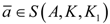 it follows that
 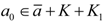 , that is,
 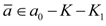 from which, since
  and a0 ∈ eff(A,K,K1) we conclude that
 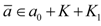 . Therefore,
  in contradiction with a0 ∉ S(A,K,K1) as claimed.
and there exists a0 ∈ eff(A,K,K1)\S(A,K,K1). From it follows that , that is, from which, since and a0 ∈ eff(A,K,K1) we conclude that . Therefore, in contradiction with a0 ∉ S(A,K,K1) as claimed.Remark 4.4
If S(A,K,K1) ≠ Ø then K + K1 = K hence eff(A,K,K1) = eff(A,K). Indeed, let a ∈ S(A,K,K1). Then, a ∈ a + K + K1 which implies that 0 ∈ K + K1.
Therefore, K ⊆ K1 + K = K1 + K ⊆ K. The above theorem shows that, for any non-empty subset of an arbitrary vector space, the set of all strong minimal elements with respect to any convex cone, through the agency of every non-void subset of it, coincides with the corresponding set of the efficient (minimal) points whenever there is at least a strong minimal element, the result remaining obviously valid for the strong maximal elements and the maximal efficient points, respectively. Using this result and our abstract construction given in [36] for the H-locally convex spaces introduced by Th. Precupanu in [37], as separated locally convex spaces with any seminorms satisfying the parallelogram law, we established in [16] that the only simultaneous and vectorial approximation for each element, in the direct sum of a (closed) linear subspace and its orthogonal with respect to a linear (continuous) operator between two H-locally convex spaces, is its spline function. We also note that it is possible to have S(A,K,K1) = Ø and eff(A,K,K1) = A. Thus, for example, if one considers X = Rn(n ∈ N, n ≥ 2) endowed with the separated H-locally convex topology generated by the semi-norms  and for each real number c we define
 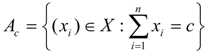 , then it is clear that S(Ac,K,K1) is empty and eff(Ac,K,K1) = Ac.
and for each real number c we define , then it is clear that S(Ac,K,K1) is empty and eff(Ac,K,K1) = Ac.In all our further considerations we suppose that X is a Hausdorff locally convex space having the topology induced by family P = {pα : α ∈ I} of seminorms, ordered by a convex cone K and its topological dual space X*. In this framework, the next theorem contains a significant criterion for the existence of the approximate Pareto (minimal) efficient points, in particular, for the usual Pareto (minimal) efficient points, taking into account that the dual cone of K is defined by K* = {x* ∈ X* : x*(x) ≥ 0, ∀x ∈ K} and its attached polar cone is K0 = −K* The version for the approximate maximal efficient points is straightforward.
Theorem 4.2
If A is any non-empty subset of X, and K1 is every non-void subset of K, then a0 ∈ eff(A,K,K1) whenever for each pα ∈ p and η ∈ (0, 1) and there exists x* in the polar cone K0 of K such that pα(a0 − a) + η, ∀a ∈ A.
Proof
Let us suppose that, under the above hypotheses, (K + K1)∩(a0 − A)⊈−(K + K1), that is, there exists a ∈ A so that a0 − a ∈ K + K1\(−K − K1) Then, a0 − a ≠ 0 and, because X is separated in Hausdorff’s sense, there exists pα ∈ p such that pα(a0 − a) > 0. On the other hand, there exists n ∈ N* sufficiently large with pα(a0 − a)/n ∈ (0, 1) and the relation given by the hypothesis of theorem leads to pα(a0 − a) ≤ x*(a0 − a) + pα(a0 − a)/n with x* ∈ K0 and n → ∞ which implies that pα(a0 − a) ≤ 0 is a contradiction and the proof is complete.
Remark 4.5
The above theorem represents an immediate extension of Precupanu’s result given in Proposition 1.2 of [38]. In general, the converse of this theorem is not valid at least in (partially) ordered separated locally convex spaces as we can see from the example considered in Remark 4.4. Indeed, if one assumes the contrary in the corresponding, mathematical calculation’s background, then, taking  it follows that for each λ0 ∈ [0, 1] there exists c1, c2 ≤ 0 such that
  . Taking
  one obtains |1 − 4λ| ≤ (c1 − c2)(1 − 4λ)+1, ∀λ ∈ [0, 1] which for λ = 0 implies that c2 ≤ c1 and for
  leads to c1 ≤ c2 that is, |1 − 4λ| ≤ 1, ∀λ ∈ [0, 1], a contradiction.
it follows that for each λ0 ∈ [0, 1] there exists c1, c2 ≤ 0 such that . Taking one obtains |1 − 4λ| ≤ (c1 − c2)(1 − 4λ)+1, ∀λ ∈ [0, 1] which for λ = 0 implies that c2 ≤ c1 and for leads to c1 ≤ c2 that is, |1 − 4λ| ≤ 1, ∀λ ∈ [0, 1], a contradiction.The content of Section 4 in [17] motivated us to consider for each function φ: P → K*\{0} the full nuclear cone Kφ = {x ∈ X : pα(x) ≤ φ(pα)(x), ∀pα ∈ p} and to give the next generalization of Theorem 7 [17] in a more general context, which represents also a new important link between strong optimization and the approximate vector optimization together with its usual particular variant, respectively.
Theorem 4.3
If there exists φ:P → K*\{0}, then,
 for any non-empty subset K1 of K.
Proof
If a0 ∈ eff(A,K,K1) is an arbitrary element, then, in accordance with point (i) of the Definition 4.1 and the hypothesis of the above theorem, we have A∩(a0 − K − K1) − a0 ⊆ K + K1 ⊆ K ⊆ Kφ for some φ:P → K*\{0}.
Therefore, a0 ∈ S(A∩(a0 − K − K1), Kφ).
Hence,  . Conversely, consider now a1 ∈ S(A∩(a0 − K − K1), Kφ) for a0 ∈ A and φ:P → K*\{0}. Then a1 ∈ A∩(a0 − K − K1) and A∩(a0 − K − K1) − a1 ⊆ Kφ, that is,
. Conversely, consider now a1 ∈ S(A∩(a0 − K − K1), Kφ) for a0 ∈ A and φ:P → K*\{0}. Then a1 ∈ A∩(a0 − K − K1) and A∩(a0 − K − K1) − a1 ⊆ Kφ, that is,pα(a − a1) ≤ φ(pα)(a − a1), ∀a ∈ A∩(a0 − K − K1), pα ∈ P which implies immediately that
pα(a − a1) ≤ −φ(pα)(a − a1) + η, ∀a ∈ A∩(a0 − K − K1), pα ∈ P, η ∈ (0, 1) and, by virtue of Theorem 4.2 one obtains that a1 ∈ eff(A∩(a0 − K − K1), K, K1).
But eff(A∩(a0 − K − K1), K, K1) ⊆ eff(A, K, K1).
Indeed, for any t ∈ eff(A∩(a0 − K − K1), K, K1) and h ∈ A∩(t − K − K1) we have h ∈ (a0 − K − K1)∩(t − K − K1) ⊆ t + K + K1 and by the point (i) of Definition 4.1 it follows that t ∈ eff(A, K, K1). This completes the proof.
Remark 4.6
The hypothesis K ⊆ Kφ imposed upon the convex cone K is automatically satisfied whenever K is an Isac’s cone and it was used only to prove the inclusion  . When K is any pointed convex cone, A is a non-empty subset of X and a0 ∈ eff(A,K) then, by virtue of (i) in Remark 4.3, it follows that A∩(a0 − K) = {a0} that is, A∩(a0 − K) − a0 = {0} ⊂ Kφ. Hence, a0 ∈ S(A∩(a0 − K), Kφ) for every mapping φ: P: K*\{0} and the next corollary is valid.
. When K is any pointed convex cone, A is a non-empty subset of X and a0 ∈ eff(A,K) then, by virtue of (i) in Remark 4.3, it follows that A∩(a0 − K) = {a0} that is, A∩(a0 − K) − a0 = {0} ⊂ Kφ. Hence, a0 ∈ S(A∩(a0 − K), Kφ) for every mapping φ: P: K*\{0} and the next corollary is valid.Corollary 4.3.1
For every non-empty subset A of any Hausdorff locally convex space ordered by an arbitrary, pointed convex cone K with its dual cone K* we have

Remark 4.7
Clearly, the announced theorem represents a significant result concerning the possibilities of scalarization for the study of the above efficiency in separated locally convex spaces, so for the particular cases of Hausdorff locally convex spaces ordered by closed, pointed and normal cones. The coincidence between the equilibrium points sets and Choquet’s boundaries together with its immediate corollaries remains valid if one replaces ε by K1.
5. Conclusions
The main goal of this paper was to exhibit some pertinent results on the equilibrium point sets for the generalized dynamical systems with respect to Isac’s cones. The relations between this kind of equilibria, the efficiency in the infinite dimensional ordered vector spaces and Choquet’s boundaries were also examined.
Acknowledgements
The author would like to thank the anonymous referees for their valuable suggestions and conclusions concerning this work.
References and Notes
- Peressini, A.L. Ordered Topological Vector Spaces; Harper and Row: New York, NY, USA, 1967. [Google Scholar]
- Isac, G. Points Critiques Pour Des Systèmes Dynamiques. In Cônes Nucleaires et Optimum de Pareto; Royal Military College of St. Jean: Québec, Canada, 1981. [Google Scholar]
- Isac, G. Sur l’existence de l’optimum de Pareto. Rivista di Matematica della Università di Parma 1983, 4, 303–325. [Google Scholar]
- Becker, R. Sur les cones faiblement comples contenus dans le dual d’un space de Banach nonreflexif. Bull. Aust. Math. Soc. 1989, 39, 321–328. [Google Scholar] [CrossRef]
- Boboc, N.; Bucur, G.H. Convex Cones of Continuous Functions on Compact Spaces; Publishing House of the Roumanian Academy: Bucharest, Romania, 1976. [Google Scholar]
- Bucur, G.H. Couples normaux de quasi-topologies. Théorèmes de prolongement. Revue Roumaine de Mathématiques Pures et Appliquées 1969, 14, 1395–1422. [Google Scholar]
- Bucur, G.H. Cônes convexes des fonctions continues sur un espace compact. Revue Roumaine de Mathématiques Pures et Appliquées 1971, 14, 1441–1460. [Google Scholar]
- Bucur, I.; Postolică, V. A coincidence results between, sets of efficient points and Choquet boundaries is separated locally convex spaces. Optimization 1996, 36, 231–234. [Google Scholar] [CrossRef]
- Choquet, G. Lecture on Analysis 1–3. In Mathematics Lecture Notes Series; Benjamin Publishing House: Benjamin, New York, Amsterdam, 1969. [Google Scholar]
- Constantinescu, C. L’ensemble des function surharmoniques positive sur un espace harmonique est faiblement complet. Comptes Rendus de l’Académie des Sciences 1970, 271, A549–A551. [Google Scholar]
- Postolică, V. Approximate efficiency in infinite dimensional ordered vector spaces. Int. J. Appl. Manag. Sci. 2009, 1, 300–314. [Google Scholar] [CrossRef]
- Bahya, A.O. Ensembles coniquement bornés et cônes nucléaires dans les éspaces localement convexes separés. Ph.D. Thesis, L’École Normale Superieure, Takaddoum Rabat, Maroc, 1989. [Google Scholar]
- Bahya, A.O. Etudes des cones nucleaires. Annales des Science Mathématique du Québec 1992, 15, 123–134. [Google Scholar]
- Isac, G. Supernormal cones and absolute summability. Libertas Mathematica 1985, 5, 17–32. [Google Scholar]
- Isac, G. Pareto optmization in infinite dimensional spaces: the importance of nuclear cones. J. Math. Anal. Appl. 1994, 182, 393–404. [Google Scholar] [CrossRef]
- Isac, G.; Postolică, V. The Best Approximation and Optimization in Locally Convex Spaces; Verlag Peter Lang Publishing House: Frankfurt am Main, Germany, 1993. [Google Scholar]
- Isac, G.; Bahya, A.O. Full nuclear cones associated to a normal cone. Application to Pareto efficiency. Appl. Math. Lett. 2002, 15, 633–639. [Google Scholar] [CrossRef]
- Postolică, V. New existence results for efficient points in locally convex spaces ordered by supernormal cones. J. Glob. Optim. 1993, 3, 233–242. [Google Scholar] [CrossRef]
- Postolică, V. An extension to sets of supernormal cones and generalized subdifferentials. Optimization 1994, 29, 131–139. [Google Scholar] [CrossRef]
- Postolică, V. Properties of Pareto sets in locally convex spaces. Optimization 1995, 34, 223–229. [Google Scholar] [CrossRef]
- Pietch, A. Nuclear Locally Convex Spaces; Springer-Verlag: Berlin, Germany, 1972. [Google Scholar]
- Krasnoselski, M.A. Positive Solutions of Operator Equations; Noordhoff Publishing House: Groningen, Noorhoff, 1964. [Google Scholar]
- Nachbin, L. Topology and Order; Van Nostrand: New York, NY, USA, 1965. [Google Scholar]
- Luc, D.T. Theory of Vector Optimization; Springer-Verlag: Berlin, Germany, 1989. [Google Scholar]
- Staib, T. On two generalizations of Pareto minimality. J. Optim. Theory Appl. 1988, 59, 289–306. [Google Scholar]
- Borwein, J.M.; Zhuang, D. Super efficiency in vector optimization. Trans. Am. Math. Soc. 1993, 338, 105–122. [Google Scholar] [CrossRef]
- Karwat, A. Sterna, on the existence of cone maximal points in real topological linear spaces. Israel J. Math. 1986, 54, 33–41. [Google Scholar] [CrossRef]
- Ha, T.X.D. On the existence of efficient points in locally convex spaces. J. Global Optim. 1994, 4, 265–278. [Google Scholar]
- Ha, T.X.D. A note on a class of cones ensuring the existence of efficient points is bounded complete sets. Optimization 1994, 31, 141–145. [Google Scholar] [CrossRef]
- Tammer, C. A generalization of Ekeland’s variational principle. Optimization 1992, 25, 129–141. [Google Scholar] [CrossRef]
- Loridan, P. ε-solutions of vector minimization problems. J. Optim. Theory Appl. 1984, 43, 65–276. [Google Scholar] [CrossRef]
- Nemeth, A.B. Near to minimality in ordered vector spaces. Mathematica 1981, 23, 239–243. [Google Scholar]
- Nemeth, A.B. Between Pareto efficiency and Pareto ε-efficiency. Optimization 1989, 20, 615–637. [Google Scholar] [CrossRef]
- Mokobodzki, G. Principe de balayage, principe de domination, Paris. Seminaire Choquet Initiation à l'analyse 1962, 1, 1–11. [Google Scholar]
- Postolică, V. Calculus of Choquet boundaries using Pareto sets. In Lecture Notes in Economics and Mathematical Systems 448; Springer-Verlag: Berlin, Germany, 1997; pp. 47–54. [Google Scholar]
- Postolică, V. Spline functions in H-locally convex spaces. Annales Scientifiques de l’Université”Al.I.Cuza.” de Jassy 1981, 27, 333–338. [Google Scholar]
- Precupanu, T. Espaces linéaires à semi-norms Hilbertiennes. Annales Scientifiques de l’Université”Al.I.Cuza.” de Jassy 1969, 115, 83–93. [Google Scholar]
- Precupanu, T. Scalar minimax properties in vectorial optimization. Numer. Math. 1992, 107, 299–306. [Google Scholar]
© 2012 by the authors; licensee MDPI, Basel, Switzerland. This article is an open access article distributed under the terms and conditions of the Creative Commons Attribution license (http://creativecommons.org/licenses/by/3.0/).