Semi-Automated Heavy-Mineral Analysis by Raman Spectroscopy

Abstract

A significant amount of information on sedimentary provenance is encoded in the heavy minerals of a sediment or sedimentary rock. This information is commonly assessed by optically determining the heavy-mineral assemblage, potentially followed by geochemical and/or geochronological analysis of specific heavy minerals. The proposed method of semi-automated heavy-mineral analysis by Raman spectroscopy (Raman-HMA) aims to combine the objective mineral identification capabilities of Raman spectroscopy with high-resolution geochemical techniques applied to single grains. The Raman-HMA method is an efficient and precise tool that significantly improves the comparability of heavy-mineral data with respect to both overall assemblages and individual compositions within solid solution series. Furthermore, the efficiency of subsequent analysis is increased due to identification and spatial referencing of the heavy minerals in the sample slide. The method is tested on modern sediments of the Fulda river (central Germany) draining two Miocene volcanic sources (Vogelsberg, Rhön) resting on top of Lower Triassic siliciclastic sediments. The downstream evolution of the volcanic detritus is documented and the capability to analyze silt-sized grains has revealed an additional eolian source. This capability also poses the possibility of systematically assessing the heavy-mineral assemblages of shales, which are often disregarded in sedimentary provenance studies.

1. Introduction

The ultimate goal of sedimentary provenance analysis is to determine source rocks and region and to infer tectonoclimatic forcing of sediment generation (e.g., [1]). Since the object of analysis has already undergone different stages and intensities of alteration during its passage from source to sink (e.g., erosion, transport and burial), the direct link between sediment grains and their source area and lithology is blurred to various degrees. The degree of modification mainly depends on processes such as weathering, hydrodynamic sorting and alteration during burial (e.g., [2,3,4,5]), and its verification and especially quantification has remained difficult. Consequently, the toolbox of sedimentary provenance analysis contains a multitude of diverse methods to extract as much information as possible from the sediment. To reduce the impact of differential fractionation, single-grain geochemical and/or isotopic techniques applied to specific mineral phases are often used which provide a tremendous toolbox in sedimentary provenance analysis and usually require electron beam or laser ablation methods. An overview of the different minerals and techniques and their discrimination potential is provided by [6,7].

Considering the variety of different minerals used for dating or chemical/isotopic analysis (14 of the most prominent ones are listed in [7]), it would be advantageous if the most informative minerals, detected during optical mineral characterization, could be directly probed by the above mentioned methods. Most of the relevant minerals used for single-grain techniques are heavy minerals. Heavy-mineral assemblages provide essential information to constrain sediment provenance (e.g., [8]) and the method has been recently revitalized using modern Raman spectroscopic techniques [9]. Thus, the main rationale of the methodology presented in this paper is to efficiently combine an improved, semi-automated Raman spectroscopic identification of heavy minerals with single-grain techniques on the same sample slide. Therefore, the sample has to be precisely characterized, i.e., the exact location and type of the heavy mineral, has to be identified, in order to (i) obtain a robust quantitative measurement of heavy-mineral proportions and (ii) pre-select minerals that are suitable for the subsequent application of single-grain techniques.

The identification of heavy minerals is conventionally done by manually using the polarizing optical microscope exploiting the optical properties of minerals. The refractive index is a key optical property and in order to estimate the refractive index of heavy minerals they are dispersed into a medium of known refractive index, usually Melt Mount^TM (n = 1.6, 1.7, ...) or Canada balm (n = 1.54). Thus, heavy minerals separates are most often prepared as strew mounts covered by a glass cover slip (see [10]). Although it is possible to extract the grains for further analyses by liquefying or dissolving the embedding medium, a more efficient approach is to prepare the sample slide in a way that it is accessible to multiple instruments. Most frequently used geochemical techniques such as electron microprobe analyses (EMPA) and laser ablation induced coupled plasma mass spectrometry (LA-ICPMS) interact with the analyte’s surface. Therefore, the grains are fixed in a competent polymer on a standard thin section glass slide and polished.

Raman spectroscopy is sensitive to molecular vibration and therefore provides information on the structure and composition of the analyte, which is why Raman spectroscopy is often used as a “finger-printing” technique to identify phases (e.g., [11]). Due to this capability Raman spectroscopy is an ideal method to automate the identification process in heavy-mineral analysis. Compared to optical microscopy Raman micro-spectroscopy has several advantages. The high lateral resolution and confocality allows the measuring of grains less than 10 µm in size. This enables quantification of the composition of silt-sized heavy minerals [12] or to characterize the inclusion inventory of different host phases (e.g., [13,14,15]). Opaque phases, which are usually neglected by optical heavy-mineral analysis, are readily identified using Raman spectroscopy. Varieties of minerals are confidently recognized [9], which eliminates the operator bias that affects the mineral identification process during optical examination. The automation potential of modern Raman microspectrometers enables the drastic increase of the number of observations (N > 1000) and, thus, decreases the counting-statistical error [16,17] relative to the usually counted 200 to 300 grains by optical mineral identification procedure. The chemical composition can be assessed semi-quantitatively. This is achieved by quantifying the shift of Raman bands with respect to mineral composition [18]. Especially cation substitution, for instance Fe, Mg, or Ca in ferromagnesian systems, give rise to significant band shifts. Such correlations have been quantified for instance for olivine [19], pyroxene [20], garnet [18,21] or amphibole [22]. Furthermore, laser-induced photo-luminescence allows the visualization of the distribution of several tri-valent rare earth elements [23] and the degree of metamictization or structural integrity can be estimated (e.g., [24,25,26]). The latter is important, for instance, to exclude metamict or structurally defected grains from geochronometric methods such as U–Pb dating (e.g., [27]). Single-grain geothermometers such as the “Zr in Rutile” thermometer [28] require knowledge about the TiO₂-polymorph under investigation, as it has been shown by [29] that detrital Rutiles are frequently mixtures or composite grains of anatase and rutile. These compositional differences are not resolved in back-scattered electron imaging, but are readily observed by Raman spectroscopy [29].

After Raman analysis it is, thus, known where which minerals are situated in the sample slide and their chemical and physical properties can be approximated to pre-select grains of interest for further geochemical and/or isotopic analysis. This approach further improves efficiency because no additional preparation of grain mounts is needed. Only the Raman mount together with the coordinates of selected minerals need to be transferred to the next in situ analytical instrument.

The proposed method was tested on series of modern sediments of the river Fulda (central Germany) and source rocks in the Fulda drainage area.

2. Methodology/Experimental

The workflow of the proposed method is as follows. (1) heavy-mineral samples are prepared as polished strew mounts as described in Section 2.1 (2) the strew mounts are photographed at high magnification in reflected and transmitted light and the topography of the strew mount is approximated as outlined in Section 2.2 (3) Adhering to the “Fleet Method” [30], measurement positions are selected by the user on the created mosaic image and the coordinate list is passed to the Raman spectrometer. Minerals are then analyzed according to their optical properties (Section 2.2). The throughput depends largely on laser power, Raman activity of the mineral and set maximum exposure time (

Table 1. A list of measurement parameters for different grain size fractions (gsf) with respect to opaque and transparent minerals. cts: counts, tTL: threshold transmitted light, tRL: threshold reflected light, fS: fine sand, cSi: coarse silt, mSi: medium silt.

Parameter	gsf:	fS (63–125 µm)	cSi (30–63 µm)	mSi (10–30 µm)
Laser wavelength (nm)	transparent	532
	opaque
Laser power (% of 100 mW)	transparent	25	25	10
	opaque	1	1	1
Laser polarization	transparent	circular (lambda/4 retarder plate)
	opaque
Spectral grating (gr/mm)	transparent	1800
	opaque
Spectrometer position (cm−1)	transparent	1000
	opaque
Spectral range (cm−1)	transparent	110–780
	opaque
Slit size (µm)	transparent	100
	opaque
Hole size (µm)	transparent	100
	opaque
Objective	transparent	50x, 0.5 NA, LWD		100x, 0.8 NA, LWD
	opaque
Maximum exposure time (s)	transparent	30		120
	opaque	300
Number of accumulations	transparent	1
	opaque	2
Maximum intensity cts	transparent	5000
	opaque	10,000
tTL (gray value 0–255)		10
tRL (gray value 0–255)		130

) and averages at ca. 400 to 500 grains per hour, but can range from ca. 1000 to 120 grains per hour. (4) The Raman spectra are automatically processed and compared to a reference database to infer the heavy-mineral assemblage, as proposed in Section 2.3. (5) Once the heavy-mineral assemblage is characterized, further insight from varieties can be gained by automated curve-fitting of mineral groups (e.g., olivine, pyroxene, garnet, etc.) to estimate chemical composition. In the following sub-sections details on the above outlined steps are presented.

2.1. Instrumental Setup

2.1.1. Raman Spectrometry

All Raman measurements were performed using the Horiba XploRA Plus system. The configuration for different measurement series is listed in Table 1.

2.1.2. Electron Microprobe Analysis (EMPA)

All EMPA measurements were performed using a Jeol JXA 8900 RL electron microprobe with a tungsten cathode as electron source. Silicates were analyzed for SiO₂, FeO, Na₂O, CaO, MgO, MnO, Cr₂O₃, NiO, Al₂O₃, and TiO₂ with an acceleration voltage of 15 kV, a probe current of 15 nA and a set beam diameter of 20 µm. Counting times were set to 15 s at each peak and 5 s for the upper and lower background, which was linearly corrected.

2.2. Sample Preparation

Using a Retsch BB 50 jaw crusher, hard rock samples (

Table 2. A list of sampling locations. VVC: Vogelsberg volcanic complex, Fsp: Feldspar.

Sample Code	N	E	Type	Note
EY55-01	50.69526	9.59377	recent sediment	Fulda river, north of VVC
EY55-02	50.50903	9.25902	Trachyte	Hard rock with weathering crust, cm-sized Fsp phenocrysts
EY55-03	50.52040	9.30481	Basalt	Hard rock with weathering crust, mm-sized olivine phenocrysts
EY55-04	50.51437	9.29809	recent sediment	Fulda tributary on VVC
EY55-05	50.53819	9.40401	recent sediment	Fulda tributary on VVC
EY55-06	50.56057	9.43914	recent sediment	Fulda tributary on VVC
EY55-07	50.45762	9.76565	recent sediment	Fulda river, south of VVC
EY55-08	50.48646	9.94867	recent sediment	near Fulda river spring, limestone gravel, not used for analysis
EY55-09	50.49809	9.93273	Basalt	Hard rock, peridotite xenoliths
EY55-10	50.49091	9.92062	Trachyte	Hard rock with weathering crust, fine grained
EY55-11	50.49251	9.92645	Basalt	Hard rock with weathering crust, fine grained, few phenocrysts
EY55-12	50.52239	9.86492	Phonolite	Hard rock, fresh
EY55-13	51.13599	9.58469	recent sediment	Fulda tributary draining only Bunter sandstone formations
EY55-14	51.21082	9.46757	recent sediment	Fulda river, most distal sample

) were iteratively crushed by setting the gap width to 4, 1.5 and 0.2 to 0.3 mm. The >500 µm fraction of the disintegrated sample was removed by manual dry sieving. The <500 µm fraction was dispersed for 15 min in an ultrasonic bath and then transferred to a wet sieving tower (Fritsch Analysette 3 Pro, 10 min run duration, amplitude 2.3 and 5 s interval time) using 250, 125, 63 and 30 µm mesh sizes, the latter being a sieve cloth and not a metal sieve. For sediment samples, the >2 mm fraction, if present, (Table 2) was removed by manual wet sieving. Afterwards, the amount of sediment was reduced to 500–600 g per sample using a riffle divider. Aggregates of silt and clay were disintegrated by 15 min of ultrasonic treatment in deionized water. In both cases (hard rock, sediment) the rinse water was collected to gain the <30 µm size fraction.

The rinse water was centrifuged to remove the <10 µm fraction. To this end the particle settling time for a grain size of 10 µm was calculated after [31] under consideration of viscosity, temperature, acceleration, tube height and tube radius [32]. The samples were centrifuged for 91 s in 800 mL tubes at 20 °C and 300 rpm (10 s acceleration and 45 s deceleration phase). After each run the supernatant was decanted and the tube refilled with water. Prior to the next run the sample was dispersed by ultrasonic treatment. This procedure was repeated until the supernatant became clear. Finally, the grain size fractions 63–125 µm (fS: fine sand), 30–63 µm (cSi: coarse silt) and 10–30 µm (mSi: medium silt) were selected for density separation.

Density separation of the fS fraction was achieved by the established funnel technique [10] using sodium polytungstate with density adjusted to 2.86–2.89 g/cm³. The samples were split by quartering to an amount of 10 to 15 g which was then loaded into the funnels. This approach, however, works poorly for the finer fractions cSi and mSi, e.g., about 70% light minerals remained in the heavy-mineral fraction after density separation. Thus, density separation of these fractions was carried out in the centrifuge. Although up to 3 g per 10 mL heavy liquid are proposed in [10], we conservatively used 1 g of sample and 40 mL of heavy liquid per centrifuge tube. Before centrifuging, the sediment was dispersed in the heavy liquid by ultrasonic treatment. Run duration was set to 5 min and fan speed to 3000 rpm. These settings ensure that a grain of 10 µm diameter will settle to the bottom of the tube. To recover the heavy minerals the lower part of the tubes was frozen by liquid nitrogen. The light minerals are then removed and after thawing of the frozen sodium polytungstate the heavy minerals could be extracted.

To analyze the heavy minerals by Raman spectrometer, EMPA, or LA-ICPMS a polished surface is crucial for the results. Therefore, the heavy minerals need to be fixed and polished. For optimal portability between the different devices the standard thin section format (48 × 28 mm) was chosen as sample carrier. The glass slide was abraded, cleaned with ethanol and placed in the oven at 50 °C to evaporate the remaining ethanol. Before mounting, the sample was split via quartering until an appropriate amount of heavy minerals remained. A flat and flexible silicon plate of 1 mm thickness is covered by double-sided adhesive foil and heavy minerals of up to 4 samples are dispersed on separated fields across the adhesive foil. A drop of ultra-violet (UV) curing glue (Uvrapid 702 by Best Klebstoffe^TM) is placed in the center of grains and the glass slide is put, with its ground surface facing towards the glue, on top of the drop. The glue is spread out between the grains by gently pressing down the glass slide. Once dispersed, the UV glue is cured by irradiating it with a UV-lamp for five minutes. Due to its flexibility the silicon layer can be easily peeled off from the glass slide.

Because the grains are already exposed to the surface, only little material needs to be removed by abrasion. To this end SiC-emery papers with 1200 and 2500 grit (for fS fraction) and 4000 grit (for mSi and cSi fractions) is used. During gentle, manual abrasion the surface is visually checked on regular basis, using a reflective microscope with 500x magnification, to ensure that a large fraction of grains is exposed to the surface. Polishing is performed iteratively on a Buehler Metaserv 2000 unit at 300 rpm, decreasing the grain size of the polishing agent after each step. Between all abrasion and polishing steps, the samples are cleaned in an ultrasonic bath. If abrasion stopped after 2500 grit, diamond polishing agents (Buehler MetaDi Monocrystalline) of grain size 9, 3, 1 µm were used. If abrasion stopped after 4000 grit, diamond polishing started at 3 µm grain size. In both cases final polishing was carried out using a water-based 0.05 µm Al₂O₃-slurry on a soft polishing cloth (Buehler MicroCloth).

During the time of preparing the manuscript we further improved the preparation routine and currently up to 20 samples can be fixed on a single glass slide which drastically increases the efficiency of this method (Figure S5). Following this approach, it takes about 1 hour to prepare a “ready-to-measure” sample slide containing up to 20 samples.

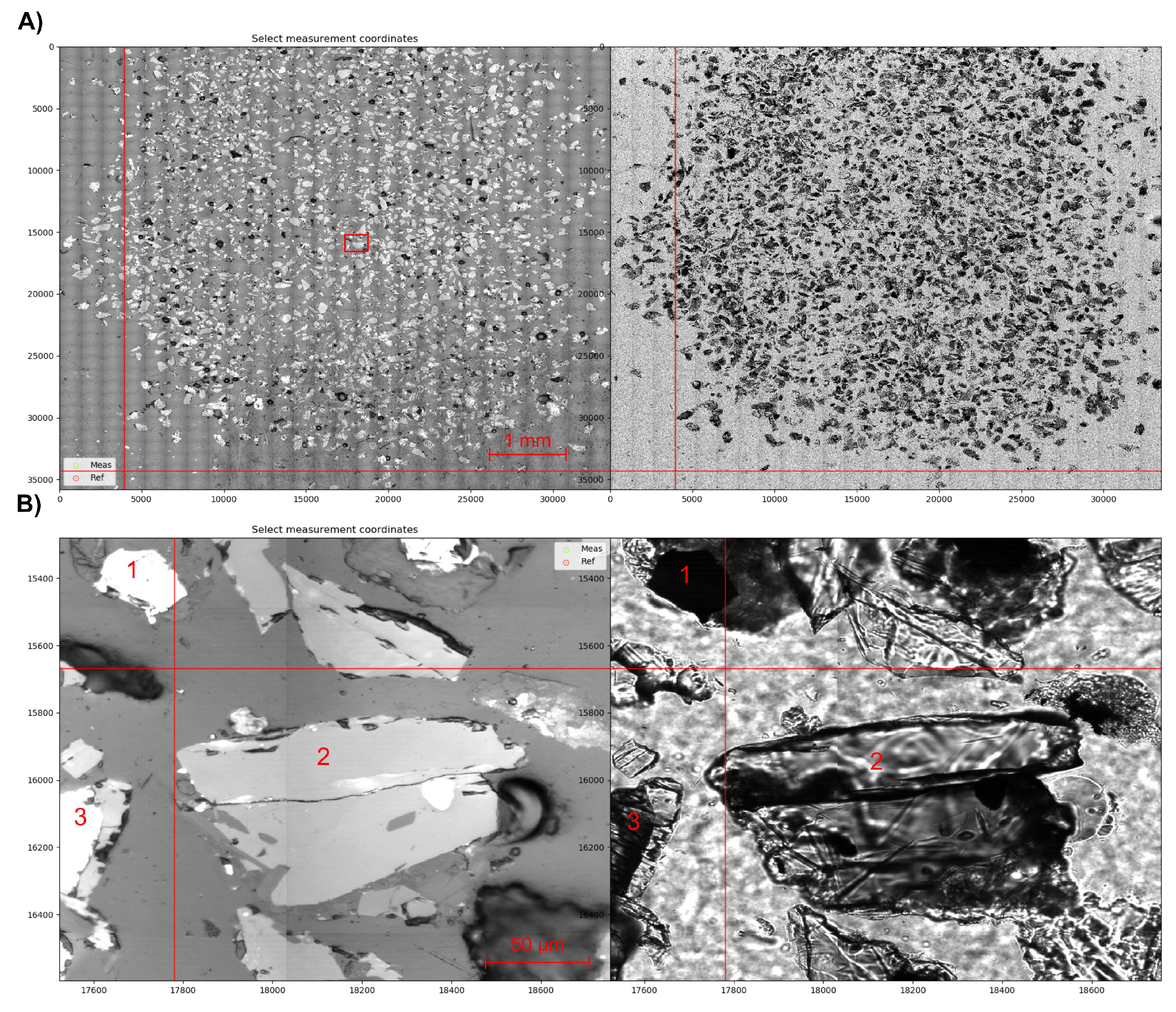
2.3. Raman Measurement Setup

Ultimately, no distinction between opaque and transparent phases is necessary for Raman analysis, as minerals of both groups are Raman active. However, to avoid photo-oxidation the opaque phases must be measured with less laser power [33,34] than the transparent phases. This requires at least two sets of measurement parameters (Table 1) and a differentiation between opaque and transparent phases before the Raman experiment, which also allows comparison of Raman-HMA data with classic optical HMA data with more confidence. Usually, a 40x or 50x objective together with a raised condenser and an inserted condenser lens is used during optical HMA to determine if a grain is opaque. Therefore, selecting measurement sites for Raman analysis should be performed under similar conditions.

Depending on grain size and grains per unit area a HM sample can cover several square centimeters on a standard thin section slide. For example, at a scaling factor of 0.22 µm/px a single image with 1292 by 968 pixels covers an area of 284.24 by 212.96 µm, which means that ca. 1645 images are needed to photograph an area of 1 cm² at high resolution (50x objective). The resulting, uncompressed mosaic image consists of 2063698560 pixels (ca. 2 Gigapixels). Depending on number of channels (red, green, blue, alpha), this is likely going to be a too large file to fit into the RAM of a typical computer and the software packages of the Raman systems often rescale the image at the expense of resolution to reduce its file size. Even if a large enough mosaic image was created within the Raman system’s software package the user would waste a significant amount of measuring time by manually selecting measurement sites because automated particle detection by means of image analysis is often not realized by the manufacturers. To satisfy these needs the Coordsetter software has been developed, which relies on the hierarchical data format (HDF). An HDF file is a versatile data container that is stored directly on the hard drive. This allows for large file sizes (>10 GB) and circumvents RAM limitations.

Before selecting measuring sites, the image data needs to be created and saved into an HDF file. The single images (tiles) of the mosaic are photographed using a Zeiss AxioImager M2m microscope with a fully motorized stage using a 50x 0.75 NA objective. The extent of the mosaic is currently defined by selecting the upper left and lower right corner of the area of interest and a focal surface is computed by interpolating through an equally distributed array of support points. At the moment 64 support points are used and at each support point the correct focus value is manually selected. Once defined, the tiles are photographed in reflected (RL) and transmitted light (TL) as gray scale images. All microscope and acquisition related information is stored in a xml file (e.g., scale factor, support point coordinates, tile extent, etc.) and after data acquisition the tiles are stitched to a mosaic that is stored as a large array in the HDF file. Together with the mosaic, the scale factor, aspect ratio, and the support point coordinates are also saved into the HDF file. As the tiles are photographed in RL and TL, two HDF files are created for one sample. The Coordsetter software allows the viewing of the mosaic at full resolution by accessing and rescaling (by default 768x768) a subset of the mosaic array. The subset is defined by the current zoom state, e.g., if totally zoomed out the whole mosaic will be rescaled to 768x768 pixels and when zooming in the subset will get smaller and smaller until full resolution is reached (Figure 1). To be able to relocate the measurement sites a framework of reference points is needed. It is good practice to set the reference points in the corners and center of the mosaic. Measurement sites are then selected by pointing and clicking. With each clicked pixel, the x-, y-, and z-coordinates, and gray values in RL and TL are registered in the output file (JavaScript Object Notation file). The z-coordinates at a given location are calculated by passing the x- and y-coordinates to a two-dimensional spline function which linearly interpolates through the support points. After storing 1000 to 2000 measurements sites, the output file, compressed mosaic image, and sample are transferred to the Raman system.

When mounted, the reference points must be relocated to be able to transfer the selected measurement coordinates into the coordinate system of the Raman-microscope stage. This is achieved by applying a rigid (Euclidean) transformation to the dataset (e.g., [35]). After transformation, the coordinate list is sorted according to the gray values in RL and TL. It is determined, based on threshold gray values (Table 1) estimated during measurement sites selection, if a grain is transparent or opaque. If the lighting during image acquisition is constant, general threshold values (tTL, tRL) could be defined. Nevertheless, an opaque grain will always show low gray values in TL and transparent grains will have relatively high gray values. Thus, tTL would be enough for discrimination; however, relatively thick and dark-colored transparent grains (rutile, Cr-spinel, etc.) will also have low gray values in TL. Compared to “real” opaques, such as Fe- or Mn-oxides, dark transparent grains will have lower gray values in RL. Using tTL in combination with tRL allows a better discrimination between opaque and transparent grains based on following relationship:

• If TL gray value >= tTL:
  ⚬ transparent grain
• If TL gray value < tTL and RL gray value < tRL:
  ⚬ transparent grain
• If TL gray value < tTL and RL gray value > tRL:
  ⚬ opaque grain
• If TL gray value < tTL:
  ⚬ opaque grain

Sorting the coordinates list by the TL gray value ensures that the measurement parameter set only must be changed once. Because the total measuring time per sample can take several hours, the temporal drift of the Raman system needs to be monitored. As proposed in [36,37] 4-Acetamidophenol was chosen as an internal standard. The average Raman band positions of this substance are reported by [38]. Before mounting the slide onto the stage, a few 4-Acetamidophenol crystals are placed on the sample surface, and after the measurement sites coordinates list has been transformed, the coordinates of the internal standard are inserted, in a user-specified interval (e.g., every 100 measurements), into the transformed coordinate list. Depending on spectral resolution, calibration routine, and temperature variation, the offset in measured and real wavenumbers can be significant and must be corrected for (see Section 2.3).

2.4. (Semi-) Automated Evaluation Routine

A recorded spectrum must be pre-processed before it can be compared to a reference material database. The pre-processing and evaluation pipeline used here thus consists of the following steps:

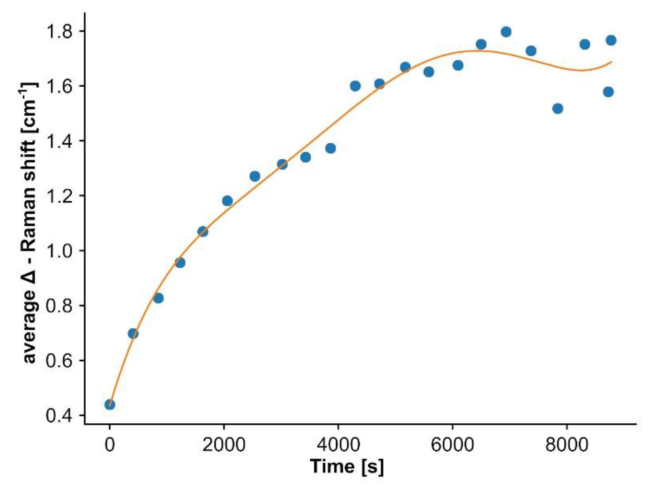
• Correcting for the temporal drift
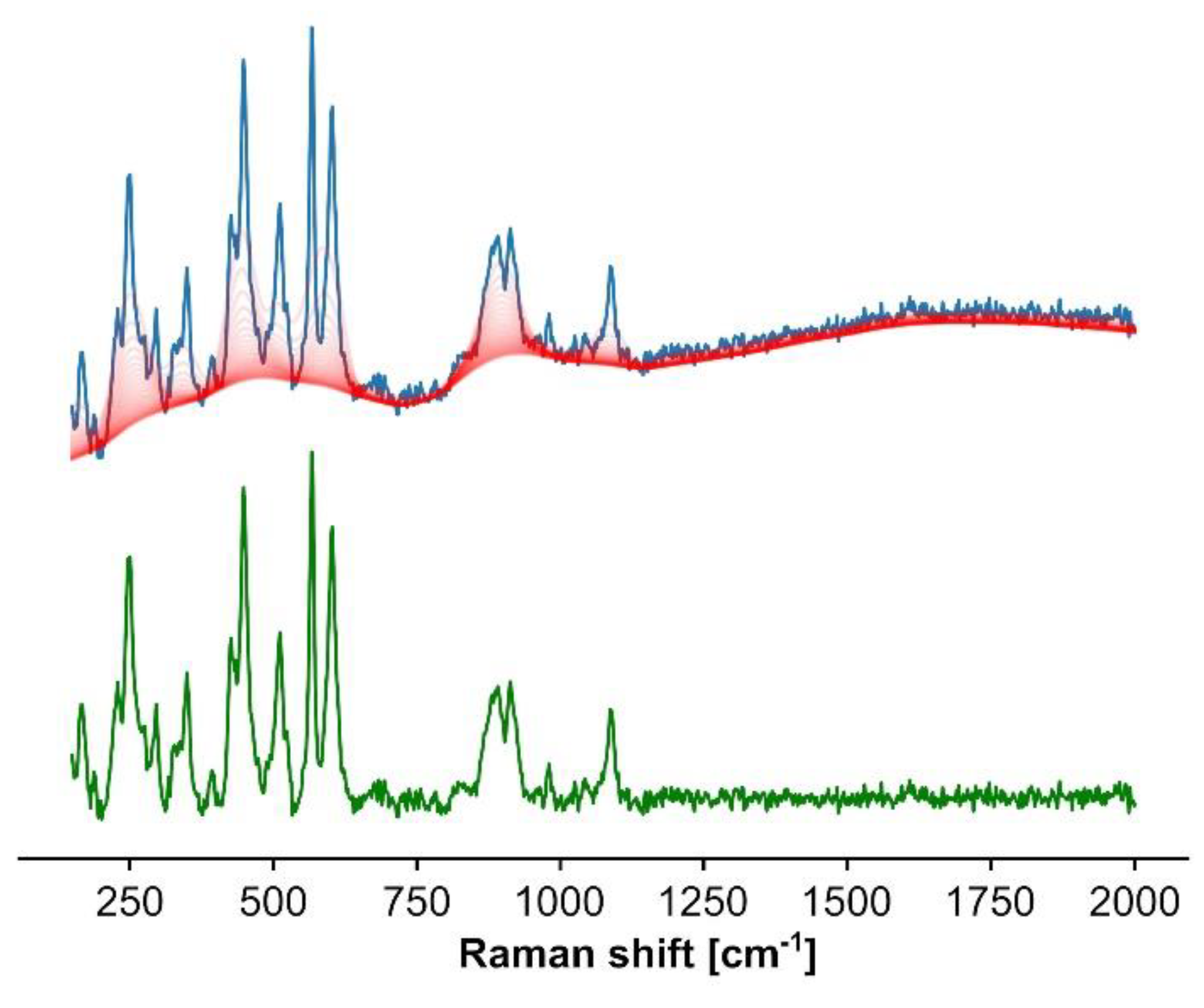
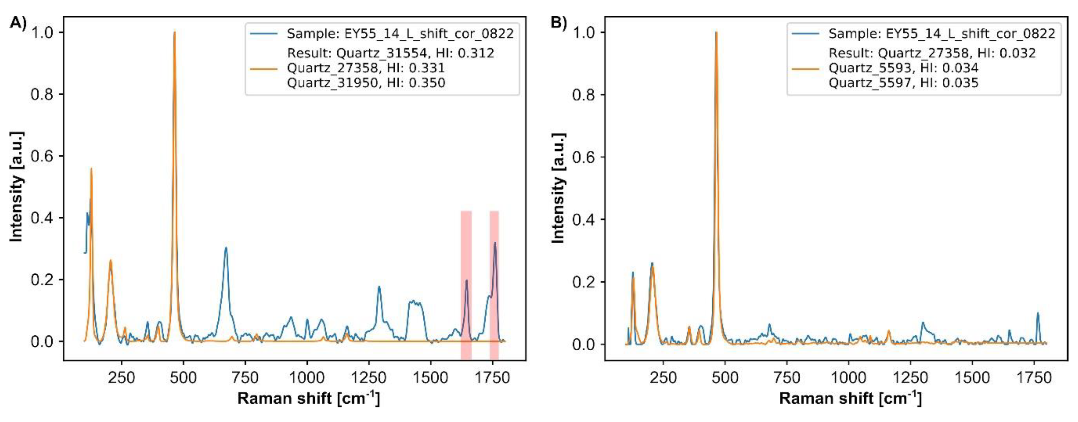
• Background removal
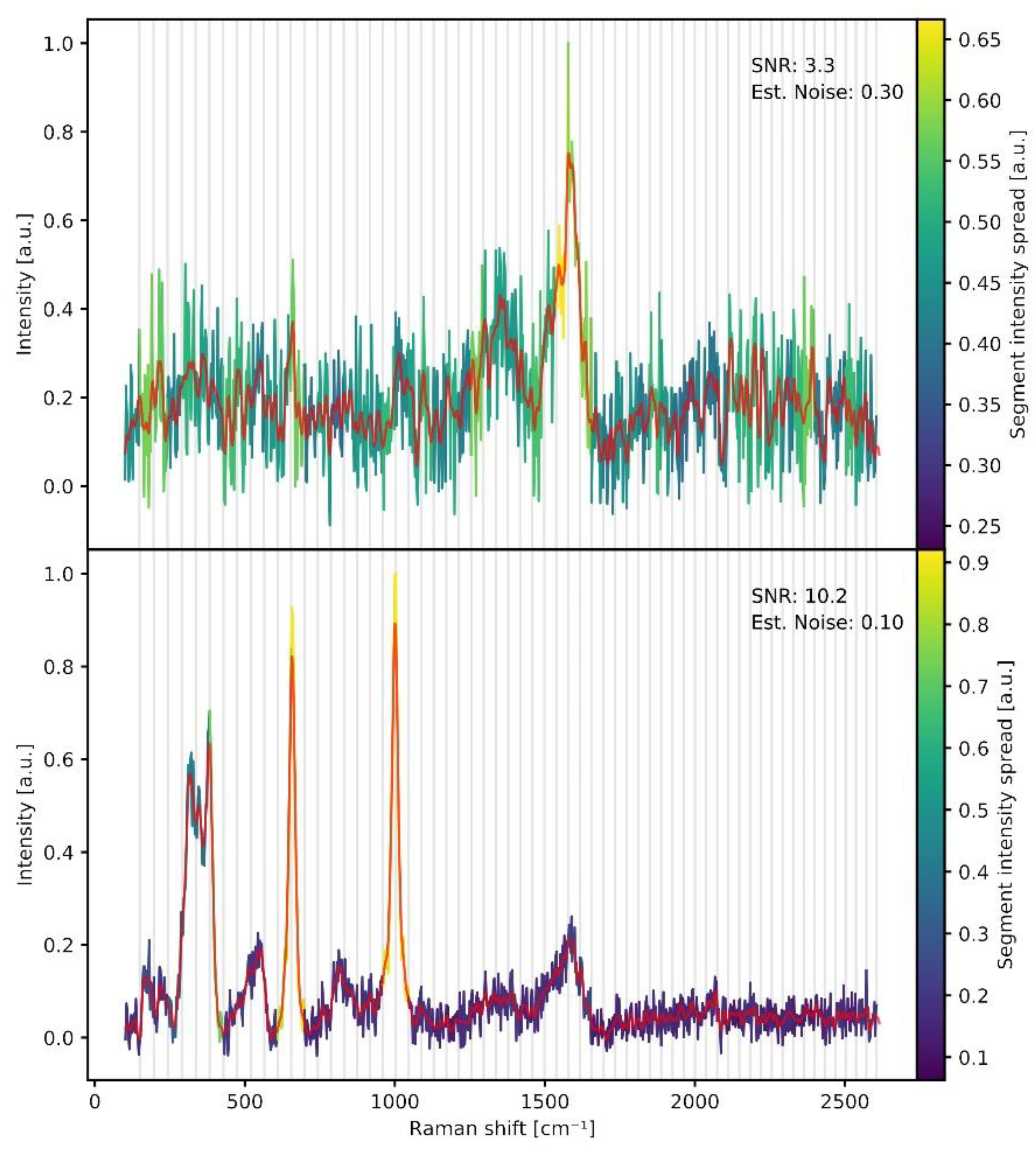
• Estimation of noise and exclusion of spectra below signal-to-noise (SNR) threshold
• Smoothing and scaling
• Correcting for embedding medium spectrum
• Phase identification and compilation of HM assemblage
• Curve-fitting of interesting mineral groups (e.g., cpx, ol, grt) to semi-quantitatively assess chemical composition

The temporal drift during a measurement session is documented by recording the spectrum of a reference material (4-Acetamidophenol) in a regular interval. For each reference spectrum the position of the Raman bands at 390.9, 651.6, 797.2, 857.9, 1168.5, 1236.8, 1278.5, 1323.9, 1371.5 and 1561.5 cm⁻¹ is determined by fitting a Lorentzian profile to the measured Raman band. The average difference between the measured and real Raman positions (avg. Δ-Raman shift) is reported for each reference spectrum. The Δ-Raman shift value is then combined with the extracted creation time of each reference spectrum file and a univariate spline is fitted through the Δ-Raman shift/creation time pairs (Figure 2). Each sample spectrum is then corrected by the Δ-Raman shift value that corresponds to its creation time.

The baseline is estimated by employing a method similar to the peak-clipping algorithm [39,40]. The Raman bands are clipped by iterative convolution of the spectrum with a Hanning window [41]. In this approach the baseline is represented by the convolution of the spectrum and a Hanning window and if an intensity value in the spectrum is higher than in the baseline, it is replaced by the baseline intensity value. Iterative application effectively removes the Raman bands (Figure 3). Iteration is terminated when a threshold value is met which is based on the decreasing difference between baselines of two consecutive iterations (Figure 3) and expressed by the squared sum of the difference. The baseline estimation depends on two parameters, namely the window size and threshold value. Both were determined empirically, and the window size is set to 0.05 times the number of datapoints in the spectrum, while the threshold value is fixed at 0.05.

The limit of detection (LOD) is given by a signal-to-noise ratio (SNR) of 3 [42]. Thus, spectra with a SNR ≤ 3 are excluded from the identification process, because they could lead to false positive results and unnecessarily extend computation time. SNR is defined as the average signal intensity above baseline divided by the standard deviation of the signal intensity [42]. This definition requires multiple accumulations, which is not advantageous for the method developed here because the total measuring time scales linearly with the number of accumulations per spectrum. Consequently, SNR must be estimated from a single accumulation and is defined here as the maximum intensity above baseline divided by the estimated noise intensity.

Any part of the spectrum that contains no Raman signal can be used to estimate the noise intensity. Because the signal-free parts of a spectrum are a priori unknown, the spectrum is divided into segments of equal length (currently 15 pxls) and the spread of intensity values is computed in each segment. If a Raman band or part of it is present in a segment the intensity spread is comparatively high. Thus, the 25th percentile of all spread values is reported as the noise intensity estimate. Because the SNR defined here is not the true SNR, the LOD is conservatively set at SNR = 10 (Figure 4).

If the spectrum satisfies the LOD condition it is smoothed and scaled. Smoothing is achieved by convoluting the baseline corrected spectrum with a Hanning window of size 9 and the spectrum is scaled to the maximum value (Figure 4).

Pre-processing is finished by correcting for Raman bands that belong to the embedding medium. These are usually epoxy resins or UV-glues that show many Raman bands in the “finger-printing region” but also contain carbonyl groups and C=C bonds which give rise to Raman intensity between 1600–1800 cm⁻¹. Inorganic minerals usually do not show Raman bands in this spectral region. Thus, two bands between 1600 and 1800 cm⁻¹ are selected in the drift corrected reference embedding medium spectra to derive a scaling factor (Figure 5). These peaks are then identified in the sample spectrum and the scaling factor specific to the sample spectrum is computed. The reference embedding medium spectrum is then multiplied by this scaling factor and subtracted from the sample spectrum (Figure 5).

Phase identification is done by comparing each sample spectrum to each spectrum in the database. Currently, the database consists of the “LR” subgroup of the RRUFF database [43]. On 28.02.2018 this subgroup contained 9433 broad scans of lower resolution (~2 cm⁻¹) which are mainly unprocessed. This group was filtered for unprocessed spectra of minerals which have been verified by at least one other method except Raman spectroscopy. The remaining 8115 spectra were extended by additional 300 spectra of confirmed heavy minerals. The latter were chosen to reflect especially the influence of metamictization in zircon and to account for luminescence bands in several phases (e.g., zircon, apatite, monazite, etc.).

$$HI=1-\frac{{\left(re{f}_m\cdot smp{l}_m\right)}^2}{\left(re{f}_m\cdot re{f}_m\right)\times \left(smp{l}_m\cdot smp{l}_m\right)}$$

(1)

The “Hit Index” (HI, Equation (1)) is computed for each pair of sample and reference spectra, where ref_m refers to the mean-centered reference spectrum, smpl_m refers to the mean-centered sample spectrum and the dot indicates vector dot products [44]. The HI is a correlation method with a success rate of ca. 80% (e.g., [45]) and ranges between 0 and 1, with 0 indicating a perfect match and 1 absolute disagreement. HI thresholds were empirically determined, and the identification results were differentiated into three groups: “Good hit” 0.0 to 0.15, “Medium hit” 0.15 to 0.3 and “No hit” for HI > 0.3. Spectra of the “Good hit” group are accepted, spectra of the “No hit” group are neglected and spectra of the “Medium hit” group should be reexamined, because these can contain correctly identified minerals, but often consist of mixed or poor quality spectra. After identification, the mineral names are sorted into a list of mineral groups approved by the International Mineralogical Association (IMA). The list (see “mineral dictionary” in the supplements) consists of mineral groups of the most common light minerals and mineral groups that contain heavy minerals, e.g., minerals with a density of 2.85 g/cm³ or higher. The output of the evaluation routine is a .csv file that contains all results, three csv files which contain the results sorted by the HI group intervals and a .png file that shows the sample spectrum with the “best hit” reference spectrum (e.g., Figure 5B).

When the phase identification is complete, Raman spectra of relevant mineral groups are selected for spectral curve fitting. Curve fitting is essential to extract Raman band parameters such as position, height, width, and area. Of these parameters, position and width convey information on crystallographic structure and mineral composition (e.g., [46]). The latter can help to further differentiate sediment sources. Curve fitting is accomplished by using the automated iterative curve-fitting approach of [47] which allows batch processing of numerous spectra with curve-fitting protocols specific for the selected mineral group.

3. Application (Case Study)

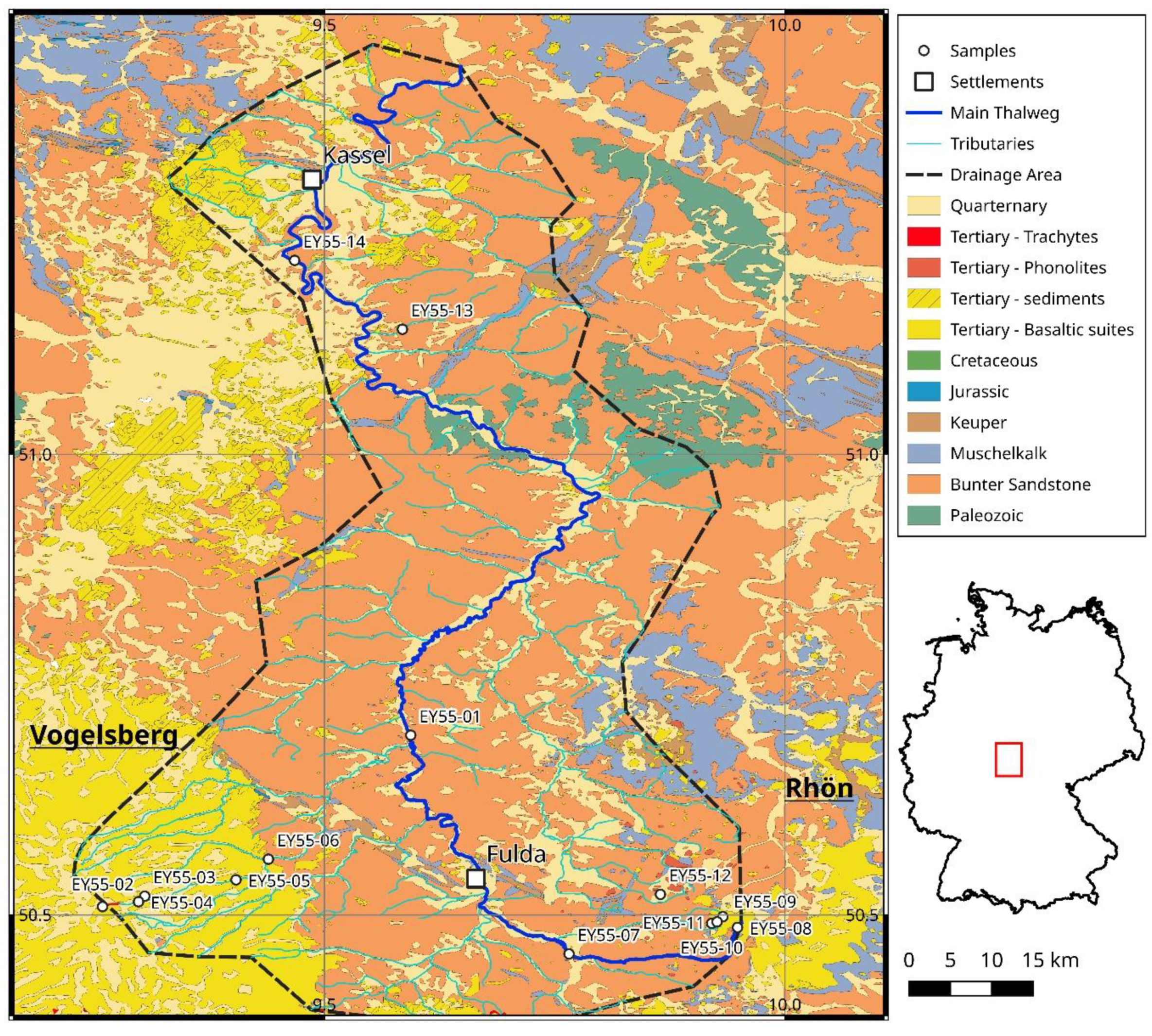
The described approach was tested on modern sediments (Table 2) of the Fulda river, a medium-sized catchment (entire river length approx. 220 km) in central Germany. The primary goal of this case study was to investigate if the heavy minerals derived from two volcanic source areas within the catchment could be traced in the modern river sediment and discriminated against the dominating siliciclastic bedrock, and if any downstream modification of the volcanic assemblages could be determined.

The Fulda drainage area (Figure 6) contains a vast proportion of Lower Triassic siliciclastic sedimentary rocks of the Bunter sandstone formation and Middle Triassic carbonates of the Muschelkalk formation. In the lower reaches of the drainage area some Permian carbonates and evaporites of the Zechstein formation and few clastic sediments of the Rotliegend formation crop out. Major occurrences of Tertiary (Miocene, 19–10 Ma) volcanic rocks are found in the Vogelsberg volcanic complex (VVC) and in the northern Rhön area at the “Wasserkuppe” close to the Fulda spring. Some more volcanic spots together with Oligocene to Miocene sediments occur further downstream in the vicinity of the city of Kassel (Figure 6). The volcanic rocks in the Fulda drainage area are mainly olivine-bearing alkali basalts and tholeiitic basalts with minor trachytes (VVC and northern Rhön) and phonolites (only northern Rhön). Quaternary deposits are dispersed across the complete drainage area and are mainly composed of loess.

A stable heavy-mineral assemblage is reported for the Bunter sandstone formation of central Germany which mostly consists of zircon and tourmaline in roughly equal proportions together with less TiO₂ minerals (rutile, anatase) and minor apatite; staurolite may occur in traces [48,49,50,51]. In general, the HM content is less than 1% and usually more than 50% of the heavy minerals are opaque phases. Similar composition and amount of heavy minerals are documented for the Permian clastic sediments [52]. The loess deposits contain higher proportions of heavy minerals (ca. 5%) and are mainly composed of amphibole, epidote and opaques in roughly equal proportions (ca. 20%) together with garnet, zircon, titanite, tourmaline, anatase (all ± 5%) and minor monazite, rutile and apatite (all <5%) and traces of spinel, sillimanite and kyanite [53]. The basalts of the VVC mainly deliver olivine and Ti–augite [54] as heavy minerals, while the heavy minerals of the trachyte consist predominantly of augitic clinopyroxene along with some titanite [55]. The volcanic rocks of the northern Rhön area provide a similar suite of heavy minerals; however, the phonolites contain significant amounts of aegirine–augite and aegirine [56].

3.1. Samples

In total 14 samples (Table 2) were collected across the Fulda river drainage area (Figure 6). The samples are divided into four groups, i.e., modern Fulda river sediments (EY55-01, -07, and -14; marked by red text in the figures), modern sediments of a Fulda tributary draining only the VVC (EY55-04, -05, and -06; marked by blue text in the figures), a modern sediment sample of a Fulda tributary draining only the Bunter sandstone formation (EY55-13; marked by violet text in the figures) and hard rock samples that depict potential source rocks (EY55-02, -03, -09, -10, -11, and -12; marked by green text in the figures). The modern Fulda river sediments were collected to reflect the downstream evolution of the heavy-mineral assemblage. EY55-07 is the most proximal sample and contains the assemblage without input from the VVC, EY55-01 is an intermediate sample containing the assemblage after the last Fulda tributary that drains the VVC and EY55-14 is the most distal sample. EY55-13 was sampled to reflect the heavy-mineral assemblage of the Bunter sandstone formation in the drainage area. Samples EY55-04 to -06 were collected to document the downstream evolution of VVC heavy-mineral assemblage.

3.2. Results

Table 3. A compilation of the results of spectral evaluation. trns: transparent, n.n.: no noise, opq: opaque, TS: total spectra, NS: noisy spectra, GH: good hit, MH: medium hit, NH: no hit, HR: hit rate, n: number of “good hit” heavy minerals. Amp: Amphibole, And: Andalusite, Ant: Anatase, Ap: Apatite, Brt: Baryte, Chm: Chamosite, Chr: Chromite, Cld: Chloritoid, Ep: Epidote, Grt: Garnet, Mag: Magnetite, Mnz: Monazite, Ol: Olivine, Opx: Orthopyroxene, Px: Pyroxene, Rt: Rutile, Sd: Siderite, Sil: Sillimanite, Spl: Spinel, St: Staurolite, Tur: Tourmaline, Ttn: Titanite, Zrn: Zircon.

Grain Size Fraction	Sample	trns	trns n.n.	opq	opq n.n.	TS	NS	GH	MH	NH	HR	Grt	Ol	Zrn	Ttn	Ep	Tur	Px	Amp	TiO2	Ap	Mnz	Other	n
fine sand	EY55-01	849	722	260	218	1109	169	478	135	110	66	0.00	13.17	16.10	0.00	0.00	5.12	59.51	0.00	4.63	0.00	0.00	1.46	410	Ttn, Amp, Spl, Brt, Ap
	EY55-02	459	411	581	572	1040	57	319	34	58	78	0.00	0.00	0.00	0.00	0.00	0.00	91.42	0.00	0.00	7.84	0.00	0.75	268	Ol, TiO2,
	EY55-03	868	725	109	97	977	155	531	68	127	73	0.00	49.90	0.00	0.00	0.00	0.00	49.33	0.00	0.00	0.00	0.00	0.77	519	Ap
	EY55-04	845	601	350	314	1195	280	338	158	105	56	0.00	14.33	0.00	0.00	0.00	0.00	83.80	0.00	0.00	0.00	0.00	1.87	321	Zrn, Ttn, Ep, Ap, Mnz
	EY55-05	1013	776	162	147	1175	252	625	66	85	81	0.00	18.11	0.00	0.00	0.00	0.00	81.40	0.00	0.00	0.00	0.00	0.49	613	Ttn, TiO2, Spl
	EY55-06	829	675	371	329	1200	196	529	77	70	78	0.00	34.04	0.00	0.00	0.00	0.00	64.22	0.00	0.00	0.00	0.00	1.74	517	Zrn, Ep, Spl, Ap
	EY55-07	562	516	441	417	1003	70	415	56	45	80	0.00	11.14	31.65	1.27	0.00	4.30	49.11	0.00	1.52	0.00	0.00	1.01	395	Ep, Amp, Spl, Mnz
	EY55-09	1012	985	4	3	1016	28	941	16	28	96	0.00	94.36	0.00	0.00	0.00	0.00	5.53	0.00	0.00	0.00	0.00	0.11	940	Ap
	EY55-10	617	566	398	361	1015	88	232	102	232	41	0.00	0.00	0.00	12.72	0.00	0.00	76.32	0.00	1.75	8.33	0.00	0.88	228	Ol, Zrn, Ep, Amp
	EY55-11	1028	991	74	74	1102	37	888	93	10	90	0.00	23.87	0.00	0.00	0.00	0.00	76.13	0.00	0.00	0.00	0.00	0.00	888	Titano-Mag
	EY55-12	766	666	262	255	1028	107	203	245	218	30	0.00	0.00	0.00	4.49	0.00	0.00	88.46	0.00	3.85	3.21	0.00	0.00	156	Mag, Feldspathoides
	EY55-13	622	600	378	378	1000	22	552	37	11	92	0.00	26.19	49.72	0.00	0.00	10.44	12.52	0.00	0.00	0.00	0.00	1.14	527	Gr, Amp, Ttn, Ant
	EY55-14	728	706	272	258	1000	36	668	18	20	95	1.40	33.33	20.00	0.00	1.75	5.61	28.42	1.05	2.46	4.21	1.05	0.70	285	Ttn, Opx, Cld, Mica, Brt
coarse silt	EY55-01	652	544	378	315	1030	171	350	112	82	64	4.28	13.90	20.32	1.07	6.42	2.14	41.71	0.00	5.88	0.00	3.74	0.53	187	Sil, St, Ap
	EY55-02	397	348	722	722	1119	49	290	33	25	83	0.00	0.00	0.00	0.00	0.00	0.00	91.44	0.00	0.00	7.78	0.00	0.78	257	Ol
	EY55-03	767	671	293	278	1060	111	561	33	77	84	0.00	42.31	0.00	0.00	0.00	0.00	56.78	0.00	0.00	0.00	0.00	0.92	546	Ap
	EY55-04	745	535	256	236	1001	230	281	140	114	53	0.00	2.25	0.00	0.00	1.87	0.00	91.39	1.12	0.00	0.00	0.00	3.37	267	Grt, Zrn, Ttn, TiO2, Ap
	EY55-05	745	507	290	274	1035	254	305	94	108	60	0.00	14.43	0.00	0.00	1.72	0.00	82.13	0.00	0.00	0.00	0.00	1.72	291	Zrn, Amp, Ap
	EY55-06	655	445	354	315	1000	249	250	81	114	56	1.27	19.92	0.00	0.00	3.81	0.00	72.03	1.27	0.00	0.00	0.00	1.69	236	Ttn, Tur, TiO2, Ap
	EY55-07	551	467	449	391	1000	142	321	80	66	69	0.00	15.71	29.49	0.00	2.88	1.60	43.27	1.28	2.56	0.00	0.00	3.21	312	Grt, Ttn, Cld, Ap, Mnz
	EY55-09	954	933	47	46	1002	22	866	31	36	93	0.00	92.12	0.00	0.00	0.00	0.00	7.76	0.00	0.00	0.00	0.00	0.12	863	Chr
	EY55-10	908	603	92	90	1000	307	284	136	183	47	0.00	0.00	0.00	0.00	0.00	0.00	97.71	0.00	0.00	1.38	0.00	0.92	218	Ttn, Titano-Mag
	EY55-11	934	910	82	81	1016	25	729	137	44	80	0.00	20.86	0.00	0.00	0.00	0.00	79.01	0.00	0.00	0.00	0.00	0.14	724	Ap
	EY55-12	931	714	81	81	1012	216	232	254	228	32	0.00	0.00	0.00	0.00	0.00	0.00	97.03	0.00	0.00	0.00	0.00	2.97	101	Ttn, Ap, Mnz, Zeo
	EY55-13	667	617	333	333	1000	50	554	41	22	90	0.00	9.81	15.09	0	22.26	6.60	36.42	4.53	1.89	1.32	0.00	2.08	530	Grt, Ttn, Sil, St, Mnz
	EY55-14	778	716	222	218	1000	66	648	44	24	91	1.23	8.62	5.23	1.54	23.69	4.00	37.54	7.38	4.92	5.54	0.00	0.31	325	St, Cld, Chm, Sd, Mnz,
medium silt	EY55-01	492	441	208	168	700	91	290	113	38	66	4.32	3.60	3.96	0.00	17.63	4.32	53.60	7.91	2.16	1.08	0.00	1.44	278	Ttn, And, St, Spl, Mnz
	EY55-02	391	386	265	265	656	5	323	42	20	84	0.00	0.00	0.00	0.00	0.00	0.00	96.85	0.00	0.00	3.15	0.00	0.00	317
	EY55-03	545	503	161	161	706	42	387	53	63	77	0.00	18.95	0.00	0.00	0.00	0.00	77.89	0.00	0.00	3.16	0.00	0.00	380
	EY55-04	486	378	214	214	700	108	214	97	67	57	0.00	2.46	1.48	0.00	5.42	0.00	86.21	1.48	0.00	0.00	0.00	2.96	203	Grt, Chm, TiO2, Ap, Mnz
	EY55-05	457	412	248	248	705	45	289	84	39	70	1.51	4.91	4.15	0.00	22.26	1.51	56.98	4.15	1.51	1.89	0.00	1.13	265	Ttn, Ky, St, Mnz
	EY55-06	448	418	164	163	612	31	260	112	46	62	0.00	2.37	1.58	0.00	5.14	0.00	85.77	1.19	0.00	3.16	0.00	0.79	253	Tur, TiO2
	EY55-07	435	397	271	269	706	40	264	81	50	67	0.00	1.54	0.00	0.00	2.70	0.00	94.21	0.00	0.00	0.00	0.00	1.54	259	Grt, Ttn, Amp, Ap
	EY55-09	1185	1131	15	15	1200	54	511	297	323	45	0.00	61.70	0.00	0.00	0.00	0.00	38.30	0.00	0.00	0.00	0.00	0.00	470
	EY55-10	481	394	221	207	702	101	178	107	109	45	0.00	0.00	0.00	0.00	0.00	0.00	93.25	3.68	0.00	0.00	0.00	3.07	163	Ol, Ep, Rt, Ap, Mnz, Titano-Mag
	EY55-11	613	600	105	96	718	22	465	80	55	78	0.00	20.53	0.00	0.00	0.00	0.00	76.85	0.00	0.00	2.39	0.00	0.24	419	Ant, Titano-Mag
	EY55-12	638	559	84	72	722	91	229	177	133	42	0.00	0.00	0.00	0.00	0.00	0.00	98.96	0.00	0.00	0.00	0.00	1.04	192	Ol, Ap, Mag, Lorenzenite
	EY55-13	488	455	217	216	705	34	366	58	31	80	3.55	2.48	12.06	0.00	25.18	4.26	32.62	10.99	6.38	1.77	0.00	0.71	282	Ttn, And
	EY55-14	496	449	207	204	703	50	385	34	30	86	4.64	2.50	8.21	1.79	25.00	2.50	33.57	13.93	3.57	1.79	2.50	0.00	280	Sil, And, St, Chm, Sd

lists all results related to the heavy-mineral assemblages determined by the method outlined in Section 2. The number of total spectra varies between 700 and 1200. Only transparent spectra with a SNR > 10 were evaluated. The difference between the number of spectra in the “Good hit” group and the number of spectra per heavy-mineral assemblage differs mainly due to the presence of light minerals, e.g., 668 “Good hit” spectra vs. 285 heavy-mineral spectra in fine sand sample EY55-14 (see “HM_result_files” in the supplements).

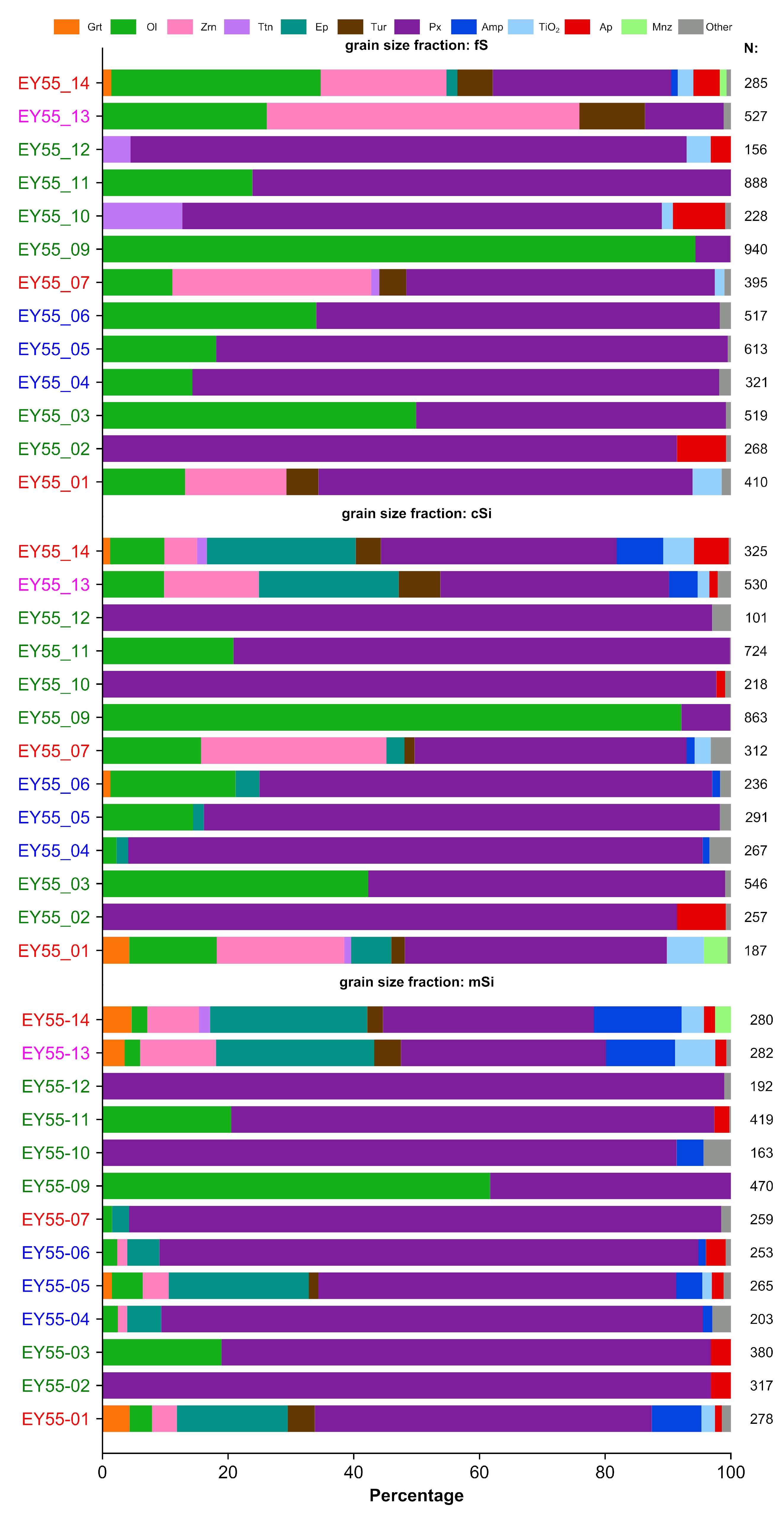
3.2.1. Heavy-Mineral Assemblages

The Fulda river sediment samples (EY55-01, 07, 14) and, interestingly, the sediments of the tributary draining only the Bunter sandstone formation (EY55-13) show a mixed provenance of the Bunter sandstone source dominated by zircon, tourmaline and rutile (ZTR) and the olivine and pyroxene rich basaltic source (Figure 7). Only the most distal sample (EY55-14) contains few garnets, epidotes, amphiboles, and apatite. Except for the latter, these phases are absent in all other samples of the fS grain size fraction. The Vogelsberg sediment samples (EY55-04, 05, 06) reflect the bimodal composition (olivine, pyroxene) of the basalts (EY55-03). The Vogelsberg trachyte (EY55-02) primarily delivers pyroxene and little apatite while the Rhön trachyte (EY55-10) additionally contains titanite. The Rhön phonolite (EY55-12) appears to be of similar composition as the Rhön trachyte, but contains many clinopyroxene grains of aegirin–augitic to aegirin composition which is not the case for the trachytes.

In all sediment samples the amount of olivine decreases with decreasing grain size while the content of epidote, amphibole and garnet increases (Figure 8). The decrease in olivine content towards finer grain size is also observed in the Vogelsberg and Rhön basalts (EY55-03, 11). Titanite even disappears in the silt fractions of the Rhön trachyte (EY55-10) and phonolite (EY55-12). Interestingly, zircon which is present in all Fulda river sediment samples in all grain size fractions, appears in the Vogelsberg sediments in the finest fractions only (Figure 7).

In the fS fraction the Ol/Px ratio of the Vogelsberg sediments (EY55-04, -06) shows a marked increase with increasing transport distance. The same is true for the modern Fulda sediments. The proximal (EY55-07) and intermediate (EY55-01) samples show similar Ol/Px ratios of less than one, while the distal sample (EY55-14) has as Ol/Px ratio of approximately one.

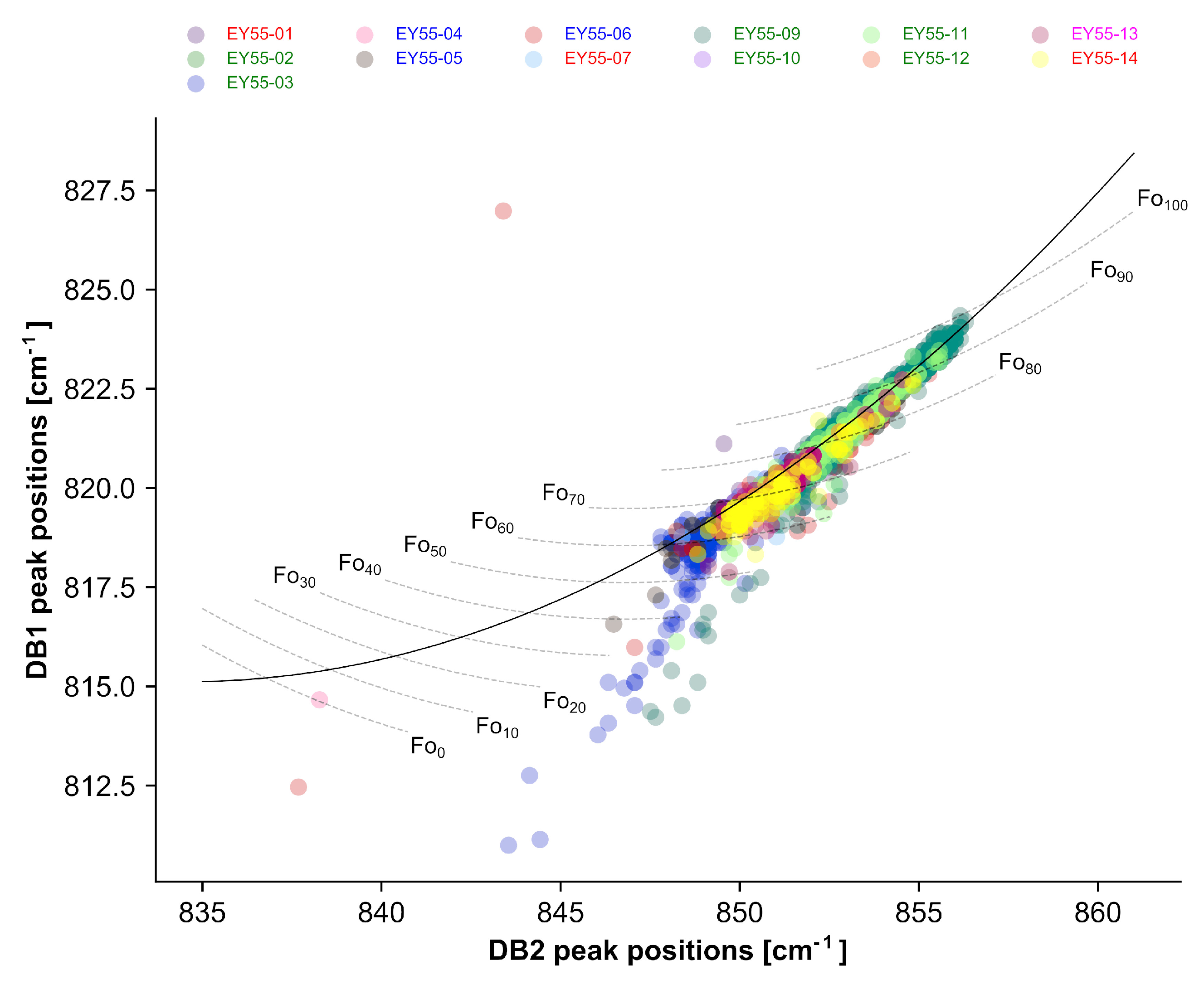
3.2.2. Semi-Quantitative Mineral Chemistry by Raman Spectroscopy: Olivine

The estimation of the content of the Mg-endmember (forsterite content) after [19] is based on the shift of two Raman bands in the olivine spectrum related to internal stretching vibrations of the SiO₄-group [57]. These bands are named DB1 and DB2 in [19] and occur at Raman shift values of ca. 820 cm^-1 and ca. 850 cm⁻¹. A suite of olivines, identified as such by the outlined approach (Methods section), were also analyzed by EMPA. The forsterite (Fo) contents estimated by Raman and EMPA range between 55% and 85% and are in good agreement within an uncertainty of ±10% Fo content for most of the analyses (blue dots in Figure 9A). However, the Fo content of several olivines with Fo content around 60% to 65% according to EMPA is severely underestimated by Raman spectroscopy (green dots in Figure 9A). The main trend in DB1 and DB2 positions of all analyzed olivines reveals a range of Fo contents between ca. 55 to 100% (Figure 10), while the hard rock basalt samples (EY55-03, -09, -11) show a second trend (Figure 10, Figure 11 and Figure S3) that deviates from the Fo content related trendline. This second trend is no longer observed in the finest grain size fraction (mSi, Figure 12) and not in any of the sediment samples (Figure 10, Figures S2 and S4).

3.2.3. Semi-Quantitative Mineral Chemistry by Raman Spectroscopy: Pyroxene

Approaches after [20,58,59] allow estimation of the chemical composition of pyroxenes in terms of Ca, Mg, and Fe content by Raman spectroscopy. The molar ratios X^Mg2+ (Mg²⁺/(Mg²⁺ + Ca²⁺ + Fe²⁺)) and X^Ca2+ (Ca²⁺/(Ca²⁺ + Mg²⁺ + Fe²⁺)) can be determined using the procedure after [20] and this method was tested on pyroxenes selected from samples EY55-01, -02, -03, and -07. To this end the chemical compositions of pyroxenes, identified by Raman spectroscopy, were determined by EMPA. Comparing the compositional results based on the procedure after [20] to EMPA results indicates that X^Mg2+ can be estimated within ±0.1 range by Raman spectroscopy and X^Ca2+ is generally overestimated by Raman spectroscopy which in turn leads to an underestimation of X^Fe2+ (Figure 13).

Therefore, only X^Mg2+ was estimated for all pyroxenes from all grain size fractions (Figure 14). The X^Mg2+ values mostly range between 0.2 and 0.5. As expected, the Mg content of pyroxenes in sediments deposited within the Vogelsberg (EY55-04, -05, -06) is the same as in the sampled basalt (EY55-03) for all analyzed grain size fractions. However, this average value is slightly higher for the coarsest fraction (ca. 0.41 vs. 0.37, Figure 14). Sediment samples of the Fulda river directly down- and up-stream of the Vogelsberg (EY55-01, -07) also provide pyroxenes with X^Mg2+ similar to the basalt sample. Pyroxenes of the sample EY55-11 (basalt, Rhön area) show X^Mg2+ values equivalent to sample EY55-03 (basalt, Vogelsberg). The higher differentiated volcanic rocks (EY55-02, -10, -12) and distal Fulda river sediments (EY55-14) contain pyroxenes with relatively less Mg. Additionally, the distal sediment samples show narrower X^Mg2+ distributions in the grain size fractions cSi and fS than all other samples. In the finest grain size fraction mSi X^Mg2+ distributions are generally narrower and the contrast between samples is less pronounced.

Besides X^Mg2+, several Raman peak positions in the pyroxene spectrum can be used to differentiate pyroxene types. By plotting the positions of peak 2 against peak 3 in the spectral region R2 and R3 (Figure 15) after [20] quadrilateral and non-quadrilateral pyroxenes are readily distinguishable. From Figure 15 it follows that a group of pyroxenes with aegirine–augitic composition is present in the Rhön phonolites (EY55-12). Interestingly, this plot also reveals that a single aegirine–augite was detected in sample EY55-01 (Fulda sediment).

4. Discussion

We will first discuss the results with respect to various aspects in the frame of the case study (Chapter 4.1 to 4.3), followed by methodological aspects including potential disadvantages and future developments (Chapters 4.4 and 4.5).

4.1. HM Assemblage

The occurrence of significant amounts of epidote and amphibole in the silt-sized fractions of the sediment samples suggest a third source that is different in composition to the Lower Triassic Bunter sandstone formation and the Miocene volcanic rocks of the Vogelsberg and Rhön. Considering (i) the exclusive occurrence of epidotes and amphiboles in the silt-sized fractions, (ii) the occurrence of epidote in all sediment samples of the drainage area including the small creeks at the flanks of the Vogelsberg volcano but in none of the volcanic hardrocks, (iii) similar pattern of amphibole occurrence with very minor exceptions (e.g., not detected in mSi faction EY55-07, present in mSi fraction of one hardrock EY55-10; Figure 7), and (iv) the widespread occurrence of Quaternary loess deposits in the drainage area, especially at the flanks of the Vogelsberg and the Rhön (Figure 6), loess appears to be the most reasonable source for silt-sized epidote and amphibole. As outlined above, the loess deposits in the drainage area contain significant amounts of amphibole and epidote in similar proportions (~20%) along with fewer garnet and zircon contents (~5%; [53]). In the silt-sized fractions the maximum amphibole, epidote, garnet and zircon contents are 14%, 25%, 5% and 12%, respectively. Considering that some silt-sized zircon most likely derives from the Bunter sandstone units, these proportions are in generally good agreement with the results after [53] and substantiate the hypothesis of a loess source.

Most olivines in the detritus have a forsterite content ranging between 50% to 100% (see Section 4.2) which translates into a range of specific gravities from 3.35 to ca. 3.8 g/cm² [60] while the clinopyroxenes have an augitic to diopsidic composition (see Section 4.3) which translates into a specific gravity of ca. 3.34 g/cm² and ca. 3.28 g/cm² [61]. Thus, the olivines and clinopyroxenes should have roughly similar settling velocities and be deposited in the same grain size window. The Ol/Px ratio in the fS grain size fraction increases with increasing transport distance (Figure 7) which points to a reduction in pyroxene compared to olivine. Possible reasons for apparent reduction of clinopyroxene could be lowering of settling velocity due to differences in grain shape or differential disintegration rates. In both cases pyroxene grains are likely to be affected more. In case of grain shape dependent settling velocity (given similar density) the olivines will probably settle faster due to a more isometric shape, while the pyroxenes would settle slower due to a more prismatic shape (see, for instance, [62,63,64]). Abrasion experiments by [65] show that in a heterogeneous mixture of basaltic components, augitic clinopyroxene is significantly faster abraded than olivine and that the average sphericity, given as the ratio of short to long axis (with 1 being a perfect sphere), during abrasion is much lower for augitic pyroxene compared to olivine, e.g., 0.65 vs. 0.8 [65]. Thus, the apparent reduction in pyroxene content during transport is probably a combined effect of differential settling velocities, with the clinopyroxenes sinking slower than the olivines, and faster disintegration of the clinopyroxenes. This is corroborated by decreasing Ol/Px ratios with decreasing grain size, as observed for most of the sediment samples, especially the most distal one, EY55-14 (Figure 7).

Sample EY55-13 was intended to reflect the heavy-mineral composition of the Bunter sandstone formation since the sampled tributary only drains this formation. However, the content of olivine and pyroxene in the heavy-mineral assemblage (Table 3 and Figure 7) points to a significant basaltic source and, thus, this sample cannot be used to infer the general Bunter sandstone heavy-mineral endmember.

4.2. Olivine Composition

The underestimation of the Fo content of some olivine is related to a shift of the DB1 and DB2 positions, which is unrelated to chemical variability (Figure 9). Optical re-examination of the respective olivine grains revealed that these grains frequently show alteration rims of iddingsite (Figure S1), which is the product of oxidative weathering of olivine and comprises a mixture of goethite and smectite [66]. Since goethite is far less translucent than the accompanied olivine, it will absorb the laser light to a much greater extent which favors heating of the iddingsitizised grain.

To test whether the observed band shifts are related to heating during measurement, an altered olivine of sample EY55-03 was selected for a series of measurements, in which laser power was the only variable (Figure 16). The spectrum recorded at 1% laser power shows several spectral features at ~200, 300, 400, 700, 1300 cm⁻¹ which likely belong to an iron hydroxide phase and the main olivine bands DB1 and DB2 are situated at 818 and 850 cm⁻¹, respectively. When increasing the laser power to 25% most spectral features disappear except DB1 and DB2, which broaden, equalize in intensity and shift to lower Raman shift values (Figure 16B). Re-measuring with 1% laser power reveals that DB1 and DB2 have shifted back to their original positions, regained their former relative intensities and their widths decreased again. Additionally, Raman bands that can be clearly related to hematite appear in the spectrum, which points to a thermally induced transformation of goethite to hematite during measurement. This transformation occurs at about 300 °C [67]. Considering this temperature as minimum, significant changes in spectral parameters of DB1 and DB2 can be explained by temperature-dependent anharmonic effects [68]. Thus, the second trend indicates the degree of heating, i.e., the larger the positional shift the higher the temperature during measurement. Because heating is to large proportion a function of absorption, the second trend theoretically reflects the amount of goethite present in the grain and therefore the degree of iddingsitization and hence the degree of olivine weathering. Interestingly, the trend related to iddingsitization in DB1 and DB2 is only observed in the crushed hard rock samples. This implies that the weathered rim is removed effectively already during erosion and early stages of fluvial transport. This conclusion is supported by the fact that sediment samples proximal to the basalt source (EY55-04, -05, -06) show nearly no iddingsitization trend in DB1 and DB2.

The primary Fo content trend probably reflects the crystallization related variability during cooling. Comparing only the basalt samples (Figure 10) shows that the Vogelsberg sample (EY55-03) contains more olivines with lower Fo content (~50–60%) than the Rhön basalts (EY55-09, -11; ~60-70%). Olivines of the sediment samples (EY55-01, -07, -14) show similar Fo content ranges (Figure 10). This indicates that the Fo content does not allow differentiation between sources in this case.

4.3. Pyroxene Composition

Estimating X^Mg2+ from the clinopyroxene Raman spectrum enables differentiation of quadrilateral pyroxenes from basic and more differentiated volcanic rocks. Here the basaltic clinopyroxenes (EY55-03, -09, -11) show median X^Mg2+ values of 0.39 (EY55-03), 0.37 (EY55-11) and 0.5 (EY55-09). The elevated X^Mg2+ value of sample EY55-09 is probably related to the presence of peridotite xenoliths that contain clinopyroxenes with higher clinoenstatite content of 49 to 63% [69] compared to the median X^Mg2+ value of xenolith-free basalt in the same area (EY55-11). The clinopyroxenes derived from the trachytes and phonolites show median X^Mg2+ values of 0.33 to 0.35 (EY55-02, -10, -12). With median X^Mg2+ values of 0.41 it is obvious that most of the clinopyroxenes in the modern sediments proximal to the Vogelsberg and Rhön (EY55-01, -07) are sourced by the basalts. However, with a median X^Mg2+ value of 0.36 the distal sediment sample (EY55-14) indicates significant contribution from lower X^Mg2+ clinopyroxenes and, thus, a more differentiated source for the clinopyroxenes. Considering the amount of trachytes and phonolites that croup out in the Fulda drainage area (Figure 6), it is improbable that such small sources, if not extremely fertile, will significantly influence the clinopyroxene composition in the distal sediment samples. A more likely explanation than a different source, is a process that selectively alters the clinopyroxene suite in the sediments. The reduction in spread of X^Mg2+ values from source rocks and proximal sediments to the distal sediments favors a process over a distinct source. Reduction of the X^Mg2+ content points towards an increase in Fe which, in case of related decrease in Ca, favors a more augitic composition. This would suggest an enrichment of augitic clinopyroxenes in the distal sediment samples. Because many clinopyroxenes of the basalt source and proximal sediments have a diopsidic composition (Figure 17), differential weathering resistance of augitic and diopsidic clinopyroxene could explain the decrease in spread and average X^Mg2+ values in the distal samples. In fact, [70] showed that the solubility of augite in water at a pH of 5–6 is about two orders of magnitude less than the solubility of diopside. Thus, it is likely that decrease of X^Mg2+ in the distal sediment samples reflects the faster dissolution of diopside during fluvial transport.

Given the fact that there are several solid solution series in the pyroxene system, for instance diopside–hedenbergite or enstatite–ferrosilite, identification of intermediate compositions by comparing complete Raman spectral traces is not precise enough, e.g., the differentiation of diopsidic or augitic clinopyroxenes is often inconclusive (Figure 18). These subtle changes in composition are better reflected by shifts in Raman band positions which allow differentiation of groups of quadrilateral pyroxenes (Figure 15, EY55-09 vs. EY55-12). Still, based on the band positions it remains unclear if the clinopyroxene is a diopside or augite, but the information that they are distinct is gained (see EMPA data and Raman band positions in Figure 18). From Figure 15 it is evident that most band positions plots on the Mg²⁺-compositional trend of quadrilateral pyroxenes, while a smaller group points towards a higher aegirine content. This smaller group is mainly made up of clinopyroxenes of sample EY55-12. The sample itself shows two distinct populations of diopsidic/hedenbergitic (low Mg²⁺) clinopyroxenes and aegirin–augitic to aegirin-rich clinopyroxenes. Within the group of aegirin–augitc clinopyroxenes few spectra of other samples can be found, indicating that these samples (EY55-01, EY55-06) contain aegirin clinopyroxene. The fact that only one aegirin–augite spectrum was detected in the sediment samples, reflects that this mineral group is present in very small amounts in the detritus. This either points to a regionally confined or an infertile source. Only the phonolites of the Rhön (EY55-12) contain aegirin–augite to larger proportions and are considered the most likely source for the detected detrital aegirin–augite. Considering that the phonolites are relatively resistant to weathering in temperate climate conditions, the source is in this case both regionally confined and infertile. Due to the increased number of observations, inherent to the proposed method, chances are higher to observe the detrital signal of such small sources. This is a major advantage, considering that the number of observations can easily be increased to further reduce the counting-statistical uncertainty.

4.4. Remarks on the Methodology and Outlook

Currently, the most severe bottleneck of the method, in terms of time, is the manual selection of measurement positions. Although user control avoids measurement positions on inclusions, grain boundaries, fractures, or polymineralic grains (lithic fragments), the time needed to select ca. 1000 grains takes about an hour. Considering that at least 1000 grains per sample should be selected and that 16–20 samples are mounted on one slide, it would take about 16 to 20 h to prepare the list of measurement positions. Thus, there is a strong need to automate this process as well. Obviously, image analysis is the method of choice; however the combination of transparent, light to dark colored to complete opaque grains in a transparent matrix is not readily solved by applying gray value threshold filters to separate the foreground from the background. We currently follow two different approaches to circumvent the problem. The first approach uses changing interference colors during rotation of perpendicular polarizers. In the other approach the pattern recognition capabilities of convoluted neural networks shall be used to identify the grains based on their shape and appearance.

The method can be further improved by reducing the number of low-quality spectra (i.e., HI values > 0.15). The majority of low-quality spectra fall into two categories, i.e., low SNR spectra and spectra affected by fluorescence. The low SNR spectra were most probably measured in an out-of-focus position. This is because the real sample surface is only approximated by interpolating through a set of support points and the local topography sometimes does not match this approximated surface. Considering that the axial resolution of confocal microscope is approximated by 1.4 × λ/(NA)² [71], where λ is the laser wavelength and NA the numerical aperture of the lens, the axial resolution of the typically used microscope objectives (100x, 0.8 NA; 50x, 0.5 NA) is, thus, ca. 1.2 µm and ca. 3 µm, respectively. Consequently, slight deviation of the local topography and approximated topography lead to a drastic reduction of Raman counts per second. Thus, it is crucial to stay in exact focus during the complete measurement series. This would decrease low SNR spectra and would speed up the measurements, because the maximum integration time could be lowered. This problem can be resolved with a dedicated focusing system that automatically readjusts the focus to the current measurement position. Such systems are commercially available. Spectra affected by fluorescence must be detected automatically, for instance by evaluating the ratio of integral intensities of the raw and baseline corrected spectrum, and marked for re-remeasuring with a different laser wavelength. This could be done while measuring. Recorded spectra will be directly evaluated/identified and marked for re-measurement with different settings (laser wavelength, accumulation time, etc.) depending on spectral quality (SNR, fluorescence).

The success rate of mineral identification using the correlation method is approximately 70% to 80% and depends significantly on the baseline estimation. If the misidentification is specific to certain phases needs to investigated, but is likely to be random. Nevertheless, the success rate must be improved and the approach after [45] will be implemented. This method is based on the discrimination capabilities of deep convolutional neural networks and appears to outmatch common comparison methods such as k-nearest neighbors (e.g., [72]), gradient boosting (e.g., [73]), random forest (e.g., [74]), support vector machines (e.g., [75,76]) or correlation (e.g., [44]) and does not require baseline estimation on which the other methods heavily rely [45].

The shortcomings outlined above can, however, be resolved and in its current state the method’s efficiency already allows a drastic increase in the number of measured grains per sample and also the number of samples per project. This implies that future sedimentary provenance studies allow the processing of higher sample numbers, which in turn results in an increased spatial and, if stratigraphically well constrained, temporal resolution. This concept could be extended to heavy minerals extracted from shales, which constitute about two thirds of the sedimentary record and contain significant amounts of heavy minerals. To date they are often inferred from bulk chemical approaches [77]. Since the Raman-HMA approach enables systematic analysis of silt-sized minerals, sedimentary provenance analysis in shales opens a promising new field of research.

4.5. Potential Disadvantages

The potentially most severe drawback of the method is that it inherently relies on spectroscopic data while optical information is, at least, partly neglected, i.e., the Raman spectrum does not convey insight on, for instance, the shape (rounded vs. non-rounded), size, color, amount of inclusions or corrosion features [78]. The high-resolution images (Figure 1) allow deduction of most of the named properties. Nevertheless, this must be done by the user, which is why stringent pairing of optical and spectroscopic data is currently not realized. In the future, this is going to be remediated with the implementation of image analysis, as outlined in Section 4.4, which can then be used to infer, for instance, color and/or shape parameters for each automatically detected grain.

The number and type of (mineral) inclusions are not readily assessed by the Raman-HMA method, but convey important information on pressure and temperature of metamorphic source rocks (e.g., [79]) or sedimentary provenance (e.g., [14]). However, the inclusion inventory can be assessed by combining the imaging capabilities of modern Raman spectrometers (e.g., [80]) with the referenced mineral positions, created by applying the Raman-HMA method. Thus, inclusions in selected minerals (e.g., garnet) can be characterized automatically by creating hyperspectral cubes at the mineral locations. These huge datasets can then be quickly screened for indicative Raman bands of, for instance, coesite or diamond.

Another inconvenience of the method is that for technical reasons, wide grain size ranges cannot be embedded within the same heavy-mineral slide. Therefore, two or more grain size fractions of one sample need to be prepared. However, this drawback is counterbalanced by the high sample throughput of the method.

5. Conclusions

With the proposed method it is now possible to assess the heavy-mineral assemblage of silt- and sand-sized sediments rapidly and with strongly increased objectivity. This is a major advantage compared to microscopical identification, which is limited by grain size and affected by the operator’s knowledge and experience of optical properties of heavy minerals. Additional discrimination potential of the Raman-HMA method arises from the capability to semi-quantitatively determine the compositions in solid solutions series, which has been shown by analyzing the forsterite content and X^Mg2+ of detrital olivine and clinopyroxene, respectively. Since all measured minerals are spatially referenced, transfer to other devices (EMPA, LA-ICPMS) is easily achieved which enables multi-approach single-grain analysis. The feasibility of this approach has been demonstrated to work by means of EMPA and Raman spectroscopy, applied to a medium-sized catchment with three component endmember mixings of Triassic siliclastics, Cenozoic volcanics, and Pleistocene loess.

References

1. Weltje, G.J.; von Eynatten, H. Quantitative provenance analysis of sediments: Review and outlook. Sediment. Geol. 2004, 171, 1–11. [Google Scholar] [CrossRef]
2. Morton, A.C.; Hallsworth, C.R. Processes controlling the composition of heavy mineral assemblages in sandstones. Sediment. Geol. 1999, 124, 3–29. [Google Scholar] [CrossRef]
3. Garzanti, E.; Andò, S.; Vezzoli, G. Grain-size dependence of sediment composition and environmental bias in provenance studies. Earth Planet. Sci. Lett. 2009, 277, 422–432. [Google Scholar] [CrossRef]
4. Garzanti, E.; Andò, S.; Limonta, M.; Fielding, L.; Najman, Y. Diagenetic control on mineralogical suites in sand, silt, and mud (Cenozoic Nile Delta): Implications for provenance reconstructions. Earth Science Rev. 2018, 185, 122–139. [Google Scholar] [CrossRef]
5. von Eynatten, H.; Tolosana-Delgado, R.; Karius, V.; Bachmann, K.; Caracciolo, L. Sediment generation in humid Mediterranean setting: Grain-size and source-rock control on sediment geochemistry and mineralogy (Sila Massif, Calabria). Sediment. Geol. 2016, 336, 68–80. [Google Scholar] [CrossRef]
6. Mange, M.A.; Morton, A.C. Geochemistry of Heavy Minerals. In Heavy Minerals in Use, 1st ed.; Mange, M.A., Wright, D.T., Eds.; Elsevier: Amsterdam, The Netherlands, 2007; pp. 345–391. [Google Scholar]
7. von Eynatten, H.; Dunkl, I. Assessing the sediment factory: The role of single grain analysis. EarthScience Rev. 2012, 115, 97–120. [Google Scholar] [CrossRef]
8. Morton, A.C.; Hallsworth, C. Identifying provenance-specific features of detrital heavy mineral assemblages in sandstones. Sediment. Geol. 1994, 90, 241–256. [Google Scholar] [CrossRef]
9. Andò, S.; Garzanti, E. Raman spectroscopy in heavy-mineral studies. Geol. Soc. London Spec. Publ. 2013, 386, 395–412. [Google Scholar] [CrossRef]
10. Mange, M.A.; Maurer, H.F.W. Schwerminerale in Farbe; Ferdinand Enke Verlag Stuttgart: Stuttgart, Germany, 1991. [Google Scholar]
11. Fries, M.; Steele, A. Raman Spectroscopy and Confocal Raman Imaging in Mineralogy and Petrography. In Confocal Raman Microscopy; Dieing, T., Hollricher, O., Toporski, J., Eds.; Springer: Berlin/Heidelberg, Germany, 2010; p. 289. [Google Scholar]
12. Andò, S.; Vignola, P.; Garzanti, E. Raman counting: A new method to determine provenance of silt. Rend. Lincei 2011, 22, 327–347. [Google Scholar] [CrossRef]
13. Korsakov, A.V.; Hutsebaut, D.; Theunissen, K.; Vandenabeele, P.; Stepanov, A.S. Raman mapping of coesite inclusions in garnet from the Kokchetav Massif (Northern Kazakhstan). Spectrochim. Acta Part A Mol. Biomol. Spectrosc. 2007, 68, 1046–1052. [Google Scholar] [CrossRef] [Green Version]
14. Schönig, J.; Meinhold, G.; von Eynatten, H.; Lünsdorf, N.K. Tracing ultrahigh-pressure metamorphism at the catchment scale. Sci. Rep. 2018, 8, 2931. [Google Scholar] [CrossRef] [PubMed] [Green Version]
15. Schönig, J.; von Eynatten, H.; Meinhold, G.; Lünsdorf, N.K. Diamond and coesite inclusions in detrital garnet of the Saxonian Erzgebirge, Germany. Geology 2019. [Google Scholar] [CrossRef]
16. Vermeesch, P. How many grains are needed for a provenance study? Earth Planet. Sci. Lett. 2004, 224, 441–451. [Google Scholar] [CrossRef]
17. Pullen, A.; Ibáñez-Mejía, M.; Gehrels, G.E.; Ibáñez-Mejía, J.C.; Pecha, M. What happens when n= 1000? Creating large-n geochronological datasets with LA-ICP-MS for geologic investigations. J. Anal. At. Spectrom. 2014, 29, 971–980. [Google Scholar] [CrossRef]
18. Smith, D.C. The RAMANITA© method for non-destructive and in situ semi-quantitative chemical analysis of mineral solid-solutions by multidimensional calibration of Raman wavenumber shifts. Spectrochim. Acta Part A Mol. Biomol. Spectrosc. 2005, 61, 2299–2314. [Google Scholar] [CrossRef] [PubMed]
19. Kuebler, K.E.; Jolliff, B.L.; Wang, A.; Haskin, L.A. Extracting olivine (Fo-Fa) compositions from Raman spectral peak positions. Geochim. Cosmochim. Acta 2006, 70, 6201–6222. [Google Scholar] [CrossRef]
20. Wang, A.; Jolliff, B.L.; Haskin, L.A.; Kuebler, K.E.; Viskupic, K.M. Characterization and comparison of structural and compositional features of planetary quadrilateral pyroxenes by Raman spectroscopy. Am. Mineral. 2001, 86, 790–806. [Google Scholar] [CrossRef]
21. Bersani, D.; Andò, S.; Vignola, P.; Moltifiori, G.; Marino, I.G.; Lottici, P.P.; Diella, V. Micro-Raman spectroscopy as a routine tool for garnet analysis. Spectrochim. Acta Part A Mol. Biomol. Spectrosc. 2009, 73, 484–491. [Google Scholar] [CrossRef]
22. Leissner, L.; Schlüter, J.; Horn, I.; Mihailova, B. Exploring the potential of Raman spectroscopy for crystallochemical analyses of complex hydrous silicates: I. Amphiboles. Am. Mineral. 2015, 100, 2682–2694. [Google Scholar] [CrossRef]
23. Lenz, C.; Nasdala, L.; Talla, D.; Hauzenberger, C.; Seitz, R.; Kolitsch, U. Laser-induced REE3+ photoluminescence of selected accessory minerals - An ‘advantageous artefact’ in Raman spectroscopy. Chem. Geol. 2015, 415, 1–16. [Google Scholar] [CrossRef]
24. Nasdala, L.; Wenzel, M.; Vavra, G.; Irmer, G.; Wenzel, T.; Kober, B. Metamictisation of natural zircon: Accumulaton versus thermal annealing of radioactivity-induced damage. Contrib. Mineral. Petrol. 2001, 141, 125–144. [Google Scholar] [CrossRef]
25. Hanchar, J.M.; Ruschel, K.; Nasdala, L.; Škoda, R.; Finger, F.; Kronz, A.; Többens, D.M.; Möller, A. A Raman spectroscopic study on the structural disorder of monazite–(Ce). Mineral. Petrol. 2012, 105, 41–55. [Google Scholar]
26. Heller, B.M.; Lünsdorf, N.K.; Dunkl, I.; Molnár, F.; von Eynatten, H. Estimation of radiation damage in titanites using Raman spectroscopy. Am. Mineral. 2019, 104, 857–868. [Google Scholar] [CrossRef]
27. Mezger, K.; Krogstad, E.J. Interpretation of discordant U-Pb zircon ages: An evaluation. J. Metamorph. Geol. 1997, 15, 127–140. [Google Scholar] [CrossRef]
28. Zack, T.; Moraes, R.; Kronz, A. Temperature dependence of Zr in rutile: Empirical calibration of a rutile thermometer. Contrib. Mineral. Petrol. 2004, 148, 471–488. [Google Scholar] [CrossRef]
29. Triebold, S.; Luvizotto, G.L.; Tolosana-Delgado, R.; Zack, T.; von Eynatten, H. Discrimination of TiO2 polymorphs in sedimentary and metamorphic rocks. Contrib. Mineral. Petrol. 2011, 161, 581–596. [Google Scholar] [CrossRef]
30. Fleet, W.F. Petrological Notes on the Old Red Sandstone of the West Midlands. Geol. Mag. 1926, 63, 505–516. [Google Scholar] [CrossRef]
31. Moore, D.M.; Reynolds, R.C. X-Ray Diffraction and the Identification and Analysis of Clay Minerals, 2nd ed.; Oxford University Press: Oxford, UK, 1997. [Google Scholar]
32. Tributh, H.; Lagaly, G. Aufbereitung und Identifizierung von Boden- und Lagerstättentonen. 1. GIT-Fachzeitschrift für das Lab. 1986, 30, 524–529. [Google Scholar]
33. de Faria, D.L.A.; Lopes, F.N. Heated goethite and natural hematite: Can Raman spectroscopy be used to differentiate them? Vib. Spectrosc. 2007, 45, 117–121. [Google Scholar] [CrossRef]
34. Hanesch, M. Raman spectroscopy of iron oxides and (oxy)hydroxides at low laser power and possible applications in environmental magnetic studies. Geophys. J. Int. 2009, 177, 941–948. [Google Scholar] [CrossRef]
35. Besl, P.J.; McKay, N.D. A Method for Registration of 3-D shapes. IEEE Trans. Pattern Anal. Mach. Intell. 1992, 14, 239–256. [Google Scholar] [CrossRef]
36. Dörfer, T.; Bocklitz, T.; Tarcea, N.; Schmitt, M.; Popp, J. Checking and improving calibration of raman spectra using chemometric approaches. Zeitschrift fur Phys. Chemie 2011, 225, 753–764. [Google Scholar] [CrossRef]
37. Popp, J.; Tarcea, N. Raman data analysis. In EMU Notes in Mineralogy, Volume 12—Applications of Raman Spectroscopy to Earth Sciences and Cultural Heritage; Dubessy, J., Caumon, M.-C., Rull, F., Eds.; European Mineralogical Union & Mineralogical Society of Great Britain & Ireland: London, UK, 2012; p. 504. [Google Scholar]
38. McCreery, R. McCreery Group—National Institute for Nanotechnology, University of Alberta, 2015. Available online: https://www.chem.ualberta.ca/~mccreery/ramanmaterials.html (accessed on 24 May 2019).
39. Ryan, C.G.; Clayton, E.; Griffin, W.L.; Sie, S.H.; Cousens, D.R. SNIP, a statistics-sensitive background treatment for the quantitative analysis of PIXE spectra in geoscience applications. Nucl. Inst. Methods Phys. Res. B 1988, 34, 396–402. [Google Scholar] [CrossRef]
40. Morháč, M.; Matoušek, V. Peak clipping algorithms for background estimation in spectroscopic data. Appl. Spectrosc. 2008, 62, 91–106. [Google Scholar] [CrossRef] [PubMed]
41. Harris, F.J. On the Use of Windows for Harmonic Analysis with the Discrete Fourier Transform. Proc. IEEE 1978, 66, 51–83. [Google Scholar] [CrossRef]
42. McCreery, R.L. Raman Spectroscopy for Chemical Analysis. In Volume 157 in Chemical Analysis—A Series of Monographs on Analytical Chemistry and Its Applications; Winefordner, J.D., Ed.; Wiley-Interscience: Hoboken, NJ, USA, 2000. [Google Scholar] [Green Version]
43. Lafuente, B.; Downs, T.R.; Yang, H.; Stone, N. The power of databases: the RRUFF project. In Highlights in Mineralogical Crystallography; Armbruster, T., Danisi, R.M., Eds.; De Greuyter: Berlin, Germany, 2015; pp. 1–30. [Google Scholar]
44. Rodriguez, J.D.; Westenberger, B.J.; Buhse, L.F.; Kauffman, J.F. Quantitative evaluation of the sensitivity of library-based Raman spectral correlation methods. Anal. Chem. 2011, 83, 4061–4067. [Google Scholar] [CrossRef] [PubMed]
45. Liu, J.C.; Osadchy, M.; Ashton, L.; Foster, M.; Solomon, C.J.; Gibson, S.J. Deep convolutional neural networks for Raman spectrum recognition: A unified solution. Analyst 2017, 142, 4067–4074. [Google Scholar] [CrossRef]
46. Nasdala, L.; Smith, D.C.; Kaindl, R.; Ziemann, M.A. Raman spectroscopy: Analytical perspectives in mineralogical research. EMU Notes Mineral. 2004, 6, 281–343. [Google Scholar]
47. Lünsdorf, N.K.; Lünsdorf, J.O. Evaluating Raman spectra of carbonaceous matter by automated, iterative curve-fitting. Int. J. Coal Geol. 2016, 160–161, 51–62. [Google Scholar] [CrossRef]
48. Sindowski, K.-H. Schüttungsrichtungen und Mineral-Provinzen im westdeutschen Buntsandstein. Geol. Jahrb. 1957, 73, 277–294. [Google Scholar]
49. Okrajek, A. Sedimentpetrographische Untersuchung toniger und sandiger Lagen des Mittleren Buntsandsteins in Bohrungen und Tagesaufschlüssen Süd-Niedersachsens. Beiträge zur Mineral. und Petrogr. 1965, 11, 507–534. [Google Scholar]
50. Heim, D. Petrographische Beitrage zur Paläogeographie des Buntsandsteins. Notizblatt des Hess. Landesamtes für Bodenforsch. zu Wiesbad. 1966, 94, 235–258. [Google Scholar]
51. Brüning, U. Stratigraphie und Lithofazies des Unteren Buntsandsteins in Südniedersachsen und Nordhessen. Geol. Jahrb. 1986, 90, 125. [Google Scholar]
52. Pryor, W.A. Petrology of the Weissliegendes sandstones in the Harz and Werra-Fulda areas, Germany. Geol. Rundsch. 1971, 60, 524–552. [Google Scholar] [CrossRef]
53. Scheffer, F.; Meyer, B.; Kalk, E. Mineraluntersuchungen am Würm-Löß südniedersächsischer Lößfluren als Voraussetzung für die Mineralanalyse verschiedener Lößbodentypen. Chem. Erde. 1958, 19, 338–360. [Google Scholar]
54. Bogaard, P.J.F.; Wörner, G. Petrogenesis of Basanitic to Tholeiitic Volcanic Rocks from the Miocene Vogelsberg, Central Germany. J. Petrol. 2003, 44, 569–602. [Google Scholar] [CrossRef] [Green Version]
55. Reischmann, T.; Schraft, A. Der Vogelsberg - Geotope im größten Vulkangebiet Mitteleuropas; Hessisches Landesamt für Umwelt und Geologie: Wiesbaden, Germany, 2009. [Google Scholar]
56. Ficke, B. Petrologische Untersuchungen an tertiären basaltischen bis phonolitschen Vulkaniten der Rhön. Mineral. Petrol. 1961, 7, 337–436. [Google Scholar] [CrossRef]
57. Chopelas, A. Single crystal Raman spectra of forsterite, fayalite, and monticellite. Am. Mineral. 1991, 76, 1101–1109. [Google Scholar]
58. Huang, E.; Chen, C.H.; Huang, T.; Lin, E.H.; Xu, J.A. Raman spectroscopic characteristics of Mg-Fe-Ca pyroxenes. Am. Mineral. 2000, 85, 473–479. [Google Scholar] [CrossRef]
59. Tribaudino, M.; Montovani, L.; Bersani, D.; Lottici, P. Raman spectroscopy of (Ca,Mg)MgSi2O6 clinopyroxenes. Am. Mineral. 2012, 97, 1339–1347. [Google Scholar] [CrossRef]
60. Mursky, G.A.; Thompson, R.M. A specific gravity index for minerals. Can. Mineral. 1958, 6, 273–287. [Google Scholar]
61. Poldervaart, A. Correlation of physical properties and chemical composition in the plagioclase, olivine and orthopyroxene series. Am. Mineral. 1950, 35, 1067–1079. [Google Scholar]
62. Komar, P.D.; Reimers, C.E. Grain shape effects on settling rates. J. Geol. 1978, 86, 193–209. [Google Scholar] [CrossRef]
63. Le Roux, J.P. Settling velocity of ellipsoidal grains as related to shape entropy. Sediment. Geol. 1996, 101, 15–20. [Google Scholar] [CrossRef]
64. Garzanti, E.; Andò, S.; Vezzoli, G. Settling equivalence of detrital minerals and grain-size dependence of sediment composition. Earth Planet. Sci. Lett. 2008, 273, 138–151. [Google Scholar] [CrossRef]
65. Cornwall, C.; Bandfield, J.L.; Titus, T.N.; Schreiber, B.C.; Montgomery, D.R. Physical abrasion of mafic minerals and basalt grains: Application to martian aeolian deposits. Icarus 2015, 256, 13–21. [Google Scholar] [CrossRef] [Green Version]
66. Smith, K.L.; Milnes, A.R.; Eggleton, R.A. Weathering of Basalt: Formation of Iddingsite. Clays Clay Miner. 1987, 35, 418–428. [Google Scholar] [CrossRef]
67. Gialanella, S.; Girardi, F.; Ischia, G.; Lonardelli, I.; Mattarelli, M.; Montagna, M. On the goethite to hematite phase transformation. J. Therm. Anal. Calorim. 2010, 102, 867–873. [Google Scholar] [CrossRef]
68. Pine, A.S.; Tannenwald, P.E. Temperature dependence of Raman linewidth and shift in α-quartz. Phys. Rev. 1969, 178, 1424–1430. [Google Scholar] [CrossRef]
69. Franz, L.; Seifert, W.; Kramer, W. Thermal evolution of the mantle underneath the Mid-German Crystalline Rise: evidence from mantle xenoliths from the Rhone area (Central Germany). Mineral. Petrol. 1997, 61, 1–25. [Google Scholar] [CrossRef]
70. Brantley, S.L.; Chen, Y. Chemical weathering rates of pyroxenes and amphiboles. In Chemical Weathering Rates of Silicate Minerals; White, A.F., Brantley, S.L., Eds.; Mineralogical Society of America: Washington, DC, USA, 1995; p. 583. [Google Scholar]
71. Dubessy, J.; Caumon, M.-C.; Rull, F.; Sharma, S. Instrumentation in Raman spectroscopy: elementary theory and practice. In EMU Notes in Mineralogy—Volume 12 Applications of Raman spectroscopy to Earth sciences and cultural heritage; Dubessy, J., Caumon, M.-C., Rull, F., Eds.; European Mineralogical Union & Mineralogical Society of Great Britain & Ireland: London, UK, 2012; pp. 83–172. [Google Scholar]
72. Cover, T.M.; Hart, P.E. Nearest Neighbor Pattern Classification. IEEE Trans. Inf. Theory 1967, 13, 21–27. [Google Scholar] [CrossRef]
73. Mason, L.; Bartlett, P.; Baxter, J.; Frean, M. Boosting Algorithms as Gradient Descent. In Advances in Neural Information Processing Systems 12; MIT Press: Cambridge, MA, USA, 2000; p. 1098. [Google Scholar]
74. Breiman, L. Random Forests. Mach. Learn. 2001, 45, 5–32. [Google Scholar] [CrossRef] [Green Version]
75. Cortes, C.; Vapnik, V. Support-Vector Networks. Mach. Learn. 1995, 297, 273–297. [Google Scholar] [CrossRef]
76. Drucker, H.; Burges, C.J.C.; Kaufman, L.; Smola, A.; Vapnik, V.; Long, W.; Nj, B. Support Vector Regression Machines. In Advances in Neural Information Processing Systems 9; MIT Press: Cambridge, MA, USA, 1996; p. 1118. [Google Scholar]
77. Totten, M.W.; Hanan, M.A. Heavy minerals in shale. In Heavy Minerals in Use; Mange, M.A., Wright, D.T., Eds.; Elsevier: Amsterdam, The Netherlands, 2007; p. 1283. [Google Scholar]
78. Andò, S.; Garzanti, E.; Padoan, M.; Limonta, M. Corrosion of heavy minerals during weathering and diagenesis: A catalog for optical analysis. Sediment. Geol. 2012, 280, 165–178. [Google Scholar] [CrossRef]
79. Kohn, M.J. “Thermoba-Raman-try”: Calibration of spectroscopic barometers and thermometers for mineral inclusions. Earth Planet. Sci. Lett. 2014, 388, 187–196. [Google Scholar] [CrossRef]
80. Zoubir, A. Raman Imaging; Springer: Berlin/Heidelberg, Germany, 2012; Volume 168. [Google Scholar]
Figure 1. (A) Overview of sample EY55-11 (grain size fraction fS) as imaged in the Coordsetter software. The left panel shows the reflected light mosaic image and the right panel the transmitted light mosaic image. The red rectangle marks the position of subfigure B. (B) Zoom-in on the mosaic image. At this zoom-level precise selection of measurement sites is possible because fine details such as inclusions at or below the surface are readily visible. The numbered grains show different stages of opacity and are used as an example on the usage of tRL and tTL. Grain 1 will be classified as an opaque grain because the TL gray value is less than tTL. With medium gray values in TL and RL, grain 2 will be classified as a transparent grain. Although the RL gray value is high, grain 3 will be classified as a transparent grain because the TL gray value is greater than tTL.
Minerals 09 00385 g001
Figure 2. Temporal drift correction. The average deviation of 10 Raman band positions of 4-Acetamidophenol from the reported band positions [38] is plotted against the measurement time. It is apparent that the temporal drift is significant, and that the system stabilized after ca. 1.5 h.
Minerals 09 00385 g002
Figure 3. Baseline estimation. The iterative nature of the baseline estimation is visualized by the faint red lines which represent intermediate baseline estimates. The green spectrum is the baseline corrected spectrum.
Minerals 09 00385 g003
Figure 4. Noise estimation. Each vertical gray bar marks a segment of the spectrum and the color bar shows the intensity spread within each segment. Segments that contain a Raman band will have a large intensity spread, while segments without Raman bands will have a low intensity spread. The 25th percentile of all intensity spread values is reported as the estimated noise. The spectrum in the upper panel would be rejected and the spectrum in the lower panel would be accepted for further processing (LOD at SNR-threshold 10).
Minerals 09 00385 g004
Figure 5. Embedding medium correction. The left panel (A) shows a composite spectrum of quartz and UV glue. Quartz is correctly identified, but the poor hit index of >0.3, due to the presence of UV-glue Raman bands, would lead to rejection of this result. A scaling factor for the UV-glue spectrum is computed based on the intensity ratio of the red shaded bands. A reference UV-glue spectrum is multiplied with the scaling factor and subtracted from the composite spectrum, leading to the corrected spectrum (right panel, B). After processing the hit index improves by an order of magnitude and the result would be accepted.
Minerals 09 00385 g005
Figure 6. Geological map of the Fulda river drainage area and sample locations. Colors refer to the stratigraphic age.
Minerals 09 00385 g006
Figure 7. Heavy-mineral assemblage of the grain size fractions mSi, cSi, and fS. N is the number of “good hit” spectra of heavy minerals and sample names are color coded to reflect Fulda river sediment samples (red), sediment samples of the Vogelsberg volcanic complex (blue) and source rock samples (green).
Minerals 09 00385 g007
Figure 8. Grain size trends. The three panels show that the content of garnet, epidote, and amphibole, given in percentage of the heavy-mineral assemblage, increases in all sediment samples with decreasing grain size.
Minerals 09 00385 g008
Figure 9. Fo content in olivines estimated by Raman spectroscopy. Panel (A) shows the forsterite content estimated from the Raman spectrum following the approach of [19] vs. electron microprobe data. The dashed lines mark the reported uncertainty of ± 0.1 for the Raman-based estimate. The green data points mark samples for which the Raman approach significantly underestimated the forsterite content. Panel (B) shows the trend in positional shift of the DB1 and DB2 Raman bands. The trend with increasing Fo content, as reported in [19], is indicated by the red line and the data points that produce Fo underestimates are shown in green.
Minerals 09 00385 g009
Figure 10. Fo content estimated by Raman spectroscopy for all samples of grain size fraction fS. The Fo content along the main trend (solid line) ranges between 55% to 100%. Only the hard rock samples (EY55-03, -09, -11, -12) contain olivines that show DB1 and DB2 positions deviating from the general Fo content trend line.
Minerals 09 00385 g010
Figure 11. Fo content estimated by Raman spectroscopy for all samples of grain size fraction cSi. The Fo content along the main trend (solid line) ranges between 55% to 85%. Only the hard rock samples (EY55-03, -09, -11, -12) contain olivines that show DB1 and DB2 positions deviating from the general Fo content trend line.
Minerals 09 00385 g011
Figure 12. Fo content estimated by Raman spectroscopy for all samples of grain size fraction mSi. The Fo content along the main trend (solid line) ranges between 50% to 100%. No clear deviating trend as in the coarser grain size fractions (Figure 10; Figure 11) is observed.
Minerals 09 00385 g012
Figure 13. Estimation of X(Mg–Ca–Fe)2+ by Raman spectroscopy and EMPA. Mg2+ and Ca2+ content was estimated following the approach of [20]. Mg2+ content is estimated reasonably well by this method, but Ca2+ content is generally underestimated. Due to the latter Fe2+ is overestimated.
Minerals 09 00385 g013
Figure 14. Boxplots of X(Mg2+) for all samples and grain size fractions. The dashed line marks the average Mg2+-content of basaltic clinopyroxenes of the Vogelsberg volcanic complex (samples EY55-03 to EY55-06) for the respective grain size fraction. The clinopyroxene phenocrysts (grain size fraction cSi and fS) of the higher differentiated rocks (EY55-02, -10, -12) show the lowest Mg2+-contents, while the spread and average Mg2+-content in the sediment samples decrease with increasing transport distance (proximal samples: EY55-01 and -07; distal sample: EY55-14). The distributions of Mg2+-contents of the matrix clinopyroxenes (grain size fraction mSi) are generally very similar.
Minerals 09 00385 g014
Figure 15. Variability of Raman peak positions for quadrilateral and non-quadrilateral pyroxenes after [20]. The positions of peak 2 and peak 3 in regions R2 and R3 (see inset A) off all clinopyroxenes (grain size fraction fS) are plotted together with average peak positions of non-quadrilateral pyroxenes. All data points plot along the Mg2+ trend of quadrilateral pyroxenes, except a group of pyroxenes of sample EY55-12 which plot close to the average aegirine values.
Minerals 09 00385 g015
Figure 16. Altered olivine spectra. Panel (A) shows a progression of Raman spectra of olivine recorded at the same position. The bottom spectrum is a composite spectrum of olivine and probably goethite at 1% laser power. The middle spectrum is recorded at 25% laser power where only the olivine Raman bands remain. The upper spectrum is again recorded at 1% laser power and is a composite of olivine and hematite (gray hematite spectrum for comparison). The gray shaded area is zoomed in panel (B). Here the positions of the DB1 and DB2 bands in olivine are marked by gray lines to demonstrate that the positional shift in DB1 and DB2 is a temporary feature at 25% laser power.
Minerals 09 00385 g016
Figure 17. Composition of pyroxenes as derived by EMPA (grain size fraction fS).
Minerals 09 00385 g017
Figure 18. Results of Raman spectral comparison vs. chemical classification. Panel (A) No distinction between diopside and augite is possible based on the hit indices, while the EMPA data clearly identifies a diopsidic composition. Panel (B) No distinction between diopside and augite is possible based on the hit indices, while the EMPA data clearly identifies an augitic composition. Although the identification using the complete spectral trace is inconclusive, the positions of peaks 2 and 3 reflect the compositional differences between the augite and diopside.
Minerals 09 00385 g018